
The Connection between the PQ Penny Flip Game and the Dihedral Groups


1
Department of Informatics, Ionian University, 7 Tsirigoti Square, 49100 Corfu, Greece
2
Department of History and Philosophy of Sciences, National and Kapodistrian University of Athens, 15771 Athens, Greece
*
Author to whom correspondence should be addressed.
†
These authors contributed equally to this work.
Mathematics 2021, 9(10), 1115; https://0-doi-org.brum.beds.ac.uk/10.3390/math9101115
Submission received: 27 April 2021
/
Revised: 11 May 2021
/
Accepted: 13 May 2021
/
Published: 14 May 2021
(This article belongs to the Section Mathematics and Computer Science)
Abstract
:This paper is inspired by the PQ penny flip game. It employs group-theoretic concepts to study the original game and its possible extensions. In this paper, it is shown that the PQ penny flip game can be associated, in a precise way, with the dihedral group and that within there exist precisely two classes of equivalent winning strategies for Q. This is achieved by proving that there are exactly two different sequences of states that can guarantee Q’s win with probability . It is demonstrated that the game can be played in every dihedral group , where , without any significant change. A formal examination of what happens when Q can draw their moves from the entire , leads to the conclusion that, again, there are exactly two classes of winning strategies for Q, each class containing an infinite number of equivalent strategies, but all of them sending the coin through the same sequence of states as before. Finally, when general extensions of the game, with the quantum player having at their disposal, are considered, a necessary and sufficient condition for Q to surely win against Picard is established: Q must make both the first and the last move in the game.
1. Introduction
It is rather unnecessary to stress the importance of game theory. It has been extensively used for decades now to help researchers and practitioners make sense of situations involving conflict, competition, and cooperation. The abstraction of players who antagonize each other in a specified framework by devising elaborate strategies has been employed in the fields of economics, political and social sciences, biology, and, naturally, computer science. Game theorists have developed an enormous technical machinery for the quantitative assessment of the players’ strategies and their pay-offs. Of particular significance is the assumption that the players are rational, which means that they seek to maximize their pay-offs. In this paper, only very basic and easy to grasp notions from game theory are used. These can be found in all standard textbooks, such as [1,2,3]. The emergence of the quantum era in information and computation also brought about the creation of the field of quantum game theory. This recent field is devoted to the study of classical games in the quantum setting, giving an exciting new perspective and results that are beyond the grasp of the classical realm.
1.1. Related Work
The year 1999 was an important milestone for the creation of the field of quantum games. In that year, two influential works were published. In a seminal paper Meyer [4] introduced the PQ penny flip game, which can be considered the quantum analogue of the classical penny flip game. The other influential work from 1999 was by Eisert et al. in [5]. There the authors presented a novel technique, known now as the Eisert–Wilkens–Lewenstein protocol, that has gained wide acceptance in the field.
In Meyer’s PQ penny flip game, the two players are the famous tv characters Picard and Q from the TV series Star Trek. They consecutively “toss” a quantum coin and if at the end of the game the coin is found heads up Q wins, otherwise Picard wins. There is a metaphor behind the two players: Picard represents the classical player and Q the quantum player. For Picard the game is perceived as the classical penny flip game, but for Q the quantumness of the coin is evident and can be exploited to their advantage. Meyer demonstrated that Q can always win with probability by employing the Hadamard operator. Afterwards, many researchers generalized this game to n-dimensional quantum systems. Important results in this direction were obtained by [6,7,8]. These results indicated that under a specific set of rules, the quantum player does have an advantage over the classical player. Nonetheless, this need not always hold as the authors in [9] pointed out. There, it was shown that if the the rules of the PQ penny flip game are appropriately modified, it is even possible that Picard may win the game. Another related problem, namely that of quantum gambling based on the Nash-equilibrium was examined in [10]. The association of every finite variant of the PQ penny flip game with finite automata, so that strategies are words accepted by the corresponding automaton, was established in [11]. In that work, the underlying assumption was that Q will always use the Hadamard operator. The present paper is also focused on the PQ penny flip game and its possible extensions, but this time without any limitations, as Q is free to choose their moves from the entire .
With respect to the Eisert–Wilkens–Lewenstein scheme, many important results have been obtained. Several quantum adaptations of the famous prisoners’ dilemma have been defined and studied, giving quantum strategies that are better than any classical strategy ([5]). Some recent results were presented in [12], where the correspondence of typical conditional strategies, used in the classical repeated prisoners’ dilemma game, to languages accepted by quantum automata was established, and in [13], where the Eisert–Wilkens–Lewenstein scheme was extended. Quantum games, especially coin tossing, have also been fruitfully utilized in many quantum cryptographic protocols. In such a setting, Alice and Bob assume the role of remote parties that, despite not trusting each other, have to agree on a random bit (see [14] and references therein). This has been extended in [15] to quantum dice rolling when multiple outcomes and parties are involved. In a different but quite similar line of thought, Parrondo games were studied via quantum lattice gas automata in [16] and in [17] it was shown that quantum automata accepting infinite words can capture winning strategies for abstract quantum games. Recently, abstract sequential quantum games were investigated in [18]. Games have been cast not only in a quantum setting, but also in a biological setting. Some well-known classical games, such as the prisoners’ dilemma, can be expressed via biological and bio-inspired concepts (see [19,20,21] for more references).
1.2. Contribution
This paper is inspired by previous research on the PQ penny flip game. Its novelty lies in the use of group-theoretic concepts to study the original game and its possible extensions. It is shown for the first time that the original PQ penny flip game can be associated in a precise way with the dihedral group . Interpreting the game in terms of stabilizers and fixed sets, which are basic and helpful group notions, facilitates the explanation and replication of Q’s strategy. Within there exist precisely two classes of winning strategies for Q. Each class contains many different strategies, but all these strategies are equivalent in the sense that they drive the coin through the same sequence of states. It is proven for the first time in the literature that there are precisely two different sequences of states that can guarantee Q’s win with probability . Subsequently, it is demonstrated that the same game can be played in the all dihedral groups , , without any significant change in the winning strategies of Q. Thus, the smallest group that captures the essence of the game is . The most general setting, where Q can draw their moves from the entire , is examined next. The definitive answer is that, perhaps surprisingly, the situation remains the same. Again, there are exactly two classes of winning strategies for Q, each class containing now an infinite number of equivalent strategies, but all of them send the coin through the same sequence of states as before. Ultimately, the original PQ penny flip game can be succinctly summarized by saying that there are precisely two paths of states that lead to Q’s win and, of course, no path that leads to Picard’s win. Finally, general extensions of the game in which Q has at their disposal, are studied. Their examination uncovers a very important fact: for Q to surely win against the classical player the tremendous advantage of available quantum actions is not enough; he must also make both the first and last move, or else he is not certain to win.
1.3. Organization
The paper is structured as follows. Section 1 sets the stage and gives the most relevant references. Section 2 introduces the notation and terminology used in this article. Section 3 proves the connection of the game with the dihedral group and Section 4 analyzes Q’s strategy in terms of group concepts. Section 5 and Section 5 analyze the characteristics and the possible extensions of the game in larger groups. A thorough discussion and evaluation of the results can be found in Section 7 and, finally, Section 8 provides a summary of the current work and sketches some ideas for future work.
2. Background
2.1. The Penny Flip Game
In what is now regarded as a landmark paper [4], Meyer defined the penny flip game between the famous television personas Picard and Q from the TV series Star Trek. From now on, for brevity, the Picard–Q game is referred to as the . This game is much more than a coin flipping game; its importance lies in the fact that it demonstrates the advantage of quantum strategies over classical strategies. The human player, Picard, can only employ classical strategies, while the quantum player, Q, is capable of using quantum strategies. This asymmetry is the reason why, no matter what Picard does, Q always wins with probability . Picard is confined to just the two classical moves available in a 2-dimensional system: he can either do nothing, or he can flip the coin. Doing nothing means that the coin remains in its current state, while flipping the coin changes its state from heads to tails or vice versa. Q’s advantage stems from the fact that he can potentially choose from an infinite pool of allowable moves; the only obvious restriction being that their move must be represented by a unitary operator. The game begins with the coin heads up and the two players act on the coin following a predetermined order. Q acts first, then Picard and last Q again. If, after Q’s last action, the coin is found heads up, then Q wins. If the coin is found tails up, then Picard wins.
In the context of the and its extensions, it is convenient to employ the terminology outlined in Definition 1, adapted from [1,3]. Informally, the word strategy implies a rational plan on behalf of each player. This plan ultimately consists of actions, or moves that the player makes as the game evolves.
Definition 1
(Winning and dominant strategies).
- A strategy is a function that associates an admissible action to every round that the player makes a move. It is convenient to represent strategies as finite sequences of moves from the player’s repertoire;
- A strategy for Picard is a winning strategy if for every strategy of Q, Picard wins the game with probability ;
- Symmetrically, a strategy for Q is a winning strategy if for every strategy of Picard, Q wins the game with probability ;
- A strategy for Picard or Q is dominated if there exists another strategy that has greater probability to win for every strategy of the other player. A strategy that dominates all other strategies is called dominant.
Of course, in the original , Picard’s strategy is just one move, e.g., . Q’s strategy on the other hand is a sequence of two moves: . Moreover, a winning strategy for Q is also a dominant strategy. Meyer proved that the use of the Hadamard operator constitutes a winning strategy for Q. If Q uses the Hadamard operator, he will win with probability , irrespective of Picard’s moves. In technical terms, the game takes place in the 2-dimensional complex Hilbert space . The computational basis of is denoted by B and consists of the kets and :
Typically, and capture the state of the coin being heads up or tails up, respectively. Picard’s moves do nothing and flip the coin correspond to the identity I and the flip operator F, respectively. As already mentioned, Q’s winning strategy is the Hadamard operator H. In the players’ moves are represented by the following matrices:
F is, of course, one of the famous Pauli matrices, frequently denoted by or . In this work the dynamics of the and its extensions are studied through the actions available to the players.
Definition 2
( moves and their composition). Let and be the sets of permissible moves for Picard and Q, respectively, and let . The set of all finite compositions of moves from M, denoted by , is called the operational space of the .
Consider for instance the composition , that can arise in the when Picard replies with F to Q’s H. A simple matrix multiplication shows that
The operational space contains not only the above operator (3), but also every operator that results from a finite composition of the moves in M. Most of them are not realized in the actual because its duration is just 3 rounds. Definition 2 can be generalized as follows:
Definition 3.
Given any game V (e.g., an extension of the original game), for which the set of moves is , its operational space is .
2.2. Dihedral Groups
The notation and definitions from group theory are based on standard textbooks such as [22,23]. The number of elements of the group G is called the order of G and is denoted by . It is customary to employ the following notation regarding powers of an arbitrary element g of a group G.
- ,
- , when , and
- , when .
The symbol ∘ of the binary operation is omitted, particularly in view of the fact that in many occasions the group elements will be represented by matrices and the operation ∘ will be matrix multiplication. Hence, instead of writing , the juxtaposition of the two elements is used.
The groups that capture the symmetries of regular polygons are called dihedral groups. By regular polygon it is understood that all the sides of the polygon have the same length and all the interior angles are equal. Furthermore, it is assumed that the center of the regular polygon is located at the origin of the plane.
Definition 4
(Dihedral groups). The group of symmetries of the regular n-gon, where , is called the dihedral group of order and is denoted by .
Many authors denote the dihedral group of order by to explicitly indicate its order. However, in this paper the notation is preferred to emphasize the geometric intuition. From now on, when referring to the arbitrary dihedral group , it will be assumed that . The group operation is composition of symmetries, i.e., composition of rotations and reflections. The symmetries of a regular n-gon, where , can be categorized as follows.
- There are also n reflection symmetries.
- –
- If n is odd these are the reflections in the lines defined by a vertex and the center of the regular n-gon. As an example, see Figure 3 depicting the reflection symmetries of the regular heptagon.
- –
- If n is even, these are reflections in the lines through opposite vertices and reflections in the lines passing through midpoints of opposite faces. An example that will play an important role in this study is given in Figure 4, showing the reflection symmetries of the regular octagon.
The general dihedral group contains the following elements (for details the interested reader may consult [22,23] or [24])
where r is the rotation by and s is any reflection. It is evident that each element of can be uniquely written as for some and l, where or 1. Elements are rotations, i.e., is the rotation by , and elements are reflections.
In particular, the dihedral group contains the 16 elements
where r is the rotation by and s is any reflection. Referring to Figure 4, s can be taken to be the reflection in the line passing through the vertices 1 and 5, or the reflection in the line passing through the midpoints A and , or the reflection in the line passing through the vertices 2 and 6, or any of the remaining reflections.
Definition 5
(Generators). Given a subset X of a group G, the smallest subgroup of G that contains X is denoted by X. The elements of X are called generators for X.
When X is finite, i.e., , as will be the case in this work, it is customary to simply write .
A typical way to specify groups is via presentations. This amounts to using generators and relations, with the understanding that all group elements can be constructed as products of powers of the generators, and the relations are equations involving the generators and the group identity. The following presentation of is especially convenient:
This presentation demonstrates that is generated by two reflections s and t. It appears in [22,25], where it is clarified that can be generated by two reflections in adjacent axes of symmetry passing though the origin and intersecting in an angle . In this case, the product is a rotation through an angle of .
3. The Connection between PQG and D8
3.1. Matrix Representations of Rotations and Reflections
A useful and quite common way to represent rotations and reflections in the plane is to use matrices. Such matrices, which are often called rotators and reflectors, can be conveniently written in a form that is easy to recognize and manipulate (see [24,26,27] for more details). A rotator representing a counter-clockwise rotation through an angle about the origin is denoted by and, similarly, a reflector about a line through the origin that makes an angle with the positive x-axis is denoted by . and are given by the formulas shown below. Note that capital R and capital S are used to designate these matrices, in order to avoid any confusion with the elements of the dihedral group that are denoted by small r and s.
It is now quite straightforward to see that the F and H operators can be written as follows.
This form reveals that both are reflectors: F reflects about a line that makes an angle with the positive x-axis. To be exact, this is the line passing through the vertices 2 and 6 in Figure 4. Likewise, H reflects about a line that makes an angle with the positive x-axis, which is the line passing through the midpoints A and in Figure 4. Hence, their axes of symmetry intersect in an angle , as shown in Figure 4. Moreover, their product , which is given in (3), is just the rotator , as can be verified by employing Formula (7). Therefore, by invoking the presentation (6), associating s to F, and t to H, or vice versa, it becomes evident that F and H generate the dihedral group . This conclusion is stated as Theorem 1.
In an effort to enhance the readability of this paper, all the proofs have been relocated to the Appendix A.
Definition 6
(The ambient group). Let V be a game with operational space . If is isomorphic to the group G, then G is called the ambient group of the game V.
Theorem 1
(The ambient group of the ). The ambient group of the is .
The above result tells us that Picard and Q’s moves generate the group . This has important ramifications. As long as the two players are allowed to use only the aforementioned actions, no matter what specific game they play, the game will take place in the group. Every conceivable composition of moves by the players is just an element of . Therefore, although the rules of the game can change dramatically, e.g., the players’ turn, the number of rounds, etc., the available moves will always be elements of .
Every element of the dihedral group can be represented by matrices of the form shown in (7) and (8) (see [23,28] or [29] for more details). One such representation is given below. In the literature it is usually referred to as the standard representation of . In more technical terms, this is a faithful irreducible representation of dimension 2. To clear any potential misunderstanding, let us emphasize that in the standard representation s corresponds to the reflection in the line passing through the vertices 1 and 5, i.e., the x-axis of Figure 4.
The above mapping of r and s uniquely determines the standard representation of the remaining reflections and rotations of .
where .
3.2. Orbits and Stabilizers
Definition 7
(Group action). Let G be a group and let X be a non-empty set. A group action ☆ of G on X is a function that satisfies the following properties.
- (A1)
- for every .
- (A2)
- , for all and all .
Under the standard representation of , its action on a state of the quantum coin is computed by simply multiplying every matrix corresponding to an element of with the ket describing the state of the coin. In what follows, in addition to speaking about an action, the expression that Gacts on X will occasionally be employed. It is convenient to just write instead of , since the action in this paper is that of operators on kets, i.e., of matrix-vector multiplication.
Definition 8
(Orbits and stabilizers). Suppose that a group G of linear operators, or their corresponding matrix representations, acts on a non-empty set of kets X. The next definitions, always taking into account that all kets of the form , with , represent ket , will be useful.
- 1.
- Given , the G-orbit of x, denoted by , is the set .
- 2.
- Given , the G-orbit of S, denoted by , is the union of the orbits , for each
- 3.
- Given , the stabilizer of x, denoted by , is the set .
- 4.
- Given , the fixed set of g, denoted by , is the set .
- 5.
- Given , the fixed set of X, denoted by , is the intersection of the fixed sets , for each .
In the next section these tools will be employed in the analysis of Q’s strategy to gain insight from a group theoretic perspective.
4. Analyzing Q’s Strategy in Terms of Groups
In this section, the is interpreted using the aforementioned groups concepts. It is helpful to use the following abbreviations, which are very common in the literature.
It is instructive to see the effect of the action of on the computational basis B. One easy way to do this is geometrically, by consulting Figure 2 and Figure 4, to see where vertices 1 and 3 are sent when being acted upon by the elements of . Alternatively, one can arrive at the same result algebraically simply by multiplying the matrix representation of every member of with and . The representations of the elements of can be readily found by setting in the more general Formulas (13) and (14). In any event, for future reference the action of on the computational basis B is summarized in Proposition 1 (recall that , with , and represent the same state).
Proposition 1
(The action of on B).
- 1.
- and have the same orbit:
- 2.
- The orbit of B is:
Q’s first move aims to drive the coin into the state
Definition 8 is helpful in understanding the advantage of Q’s move in terms of group notions. In particular, there are certain elements of whose action on has no effect whatsoever and which constitute the stabilizer of . These can be easily found either geometrically or algebraically, and are listed in Proposition 2.
Proposition 2
(The stabilizers of and in ).
- The stabilizers of and in are
- The stabilizers of and are
In a complementary manner, it can be surmised that Picard’s set of moves fixes specific states in , as demonstrated in Proposition 3.
Proposition 3
(The fixed set of in ).
- 1.
- The fixed set of F in is the set
- 2.
- The fixed set of in is the set
Proposition 2 tells us that Picard’s set of moves is a subset of and Proposition 3 completes the picture by revealing that ket is among those that are fixed by Picard’s moves. Thus, he is completely powerless to change the state of the coin. From this perspective the progression of the can be abstractly described as by the following “algorithm”.
Picard symbolizes the classical player and as such it is quite appropriate to assume that their repertoire is the set . This set is also a group, in particular the group of two elements (In the literature is more often denoted as under addition modulo 2). In the rest of this paper it will be assumed that the classical player can only make use of these two actions. In the coming sections Algorithm 1 will be employed to discover winning strategies for Q in more general situations.
| Algorithm 1: Q’s Winning Strategy. |
|
5. Enlarging the Operational Space of the Game
The operational space of the original is indeed a group, and, in particular, the dihedral group , as established by Theorem 1. In this section, the ambient group of the will be progressively enlarged and Q’s winning strategies will be analyzed. The analysis is guided by the belief that the essence of the original is the sharp distinction between the classical and the quantum player. From this perspective, the subsequent investigation relies on the following two assumptions.
- Picard, who embodies the classical player, can flip the coin. If he is deprived of this ability, then the resulting game becomes trivial and meaningless. He should not be able to do more than that, as this would endow them with quantum capabilities. Formally, this is expressed by specifying:
- Q, who stands for the quantum player, must exhibit quantumness. Thus, at least one of their actions must lie outside the classical realm. In more technical terms, their repertoire must contain at least one operator from other than I and F.
Under the above assumptions, the following properties are observed. These properties are quite general, as they are satisfied by every winning strategy of Q, no matter what the ambient group is. Therefore, they will be invoked when much larger dihedral groups and the unitary group are considered.
Theorem 2
(Characteristic properties of winning strategies). If is a winning strategy for Q, then:
The notion of equivalent strategies greatly simplifies the classification of winning strategies. Two strategies are considered to be equivalent if, when acting on the same initial state of the coin, they produce the same sequence of states. In view of the extension of the original game that will be undertaken in Section 6, the next definition is general enough to deal with strategies for games with more than three number of rounds.
Definition 9
(Equivalent strategies). Let and be two strategies of the same player, and let be the initial state of the coin. σ and are equivalent with respect to , denoted by , if
Q’s strategies and are equivalent because they send the coin from state first to and then back to . It is obvious that ∼ is an equivalence relation that partitions the set of strategies into equivalence classes of strategies.
Definition 10
(Strategy classes).
- 1.
- Given a strategy σ, designates the equivalence class that contains σ. Any member of is a representative of .
- 2.
- To every class the state path is associated as follows: if is any representative of , is defined to be , where
Clearly, the state path is well-defined and unique for each class . The equivalence class contains 16 strategies, as will be explained in Example 1, and the corresponding state path is .
5.1. Inside
Before delving into larger groups, the case where Q can chose their moves from the entire group is examined, i.e.,
The following Example 1 will be instructive.
Example 1.
In this example, Algorithm 1 facilitates the study all winning strategies of Q in the original . Let be Q’s first and second move in a winning strategy. After Q’s first move the quantum coin will in one of the states in the orbit , where B is the computational basis. From (18) it follows that .
- Let us first establish that if Q leaves the coin at state , or sends it to state , then he will not be able to win with probability . To see this more clearly, let us recall that, by Theorem 2, . If leaves the coin at state , i.e., , then , which is impossible because represents an element of . The same reasoning shows that if Q’s first move sends the coin to state , then he will not be able to win with probability .
- In the original , Q won by sending the coin to state . In , this can be achieved with 4 different ways: , and . State is fixed by I and F according to (23), which means that no matter what Picard plays, the coin will remain in this state. Finally, Q can send the coin back to the state with 4 different ways: , and . This means that Q has 16 different winning strategies, which, in view of Definition 9, are equivalent. Thus, they constitute one equivalence class of winning strategies. Strategy is a representative of this class, but any other strategy would also do. For this class the corresponding state path is .
- Algorithm 1 enables us to discover one more winning strategy for Q. Q has another option, which is to drive the coin to state . This can also be achieved with 4 different ways: , or . Picard cannot change this state either because is fixed by I and F, according to (23). During the final round Q has the opportunity to send the coin back to the state with 4 different ways: , or . Hence, Q has 16 more winning strategies, which are equivalent. They make the second equivalence class of winning strategies and any one of them, e.g., can be its representative. For this class, the corresponding state path is .
- Picard, unfortunately for him, has no winning strategy.
According to Definition 1, for Q a winning strategy is also a dominant strategy. Hence, Q has precisely two classes of winning and dominant strategies, each containing 16 individual strategies. These two classes correspond to exactly the 2 path states , and . ◃
Theorem 3.
(The ambient group of the is ). If and , i.e., the ambient group of the is , then the following hold.
- 1.
- Q has exactly two classes of winning and dominant strategies, each containing 16 equivalent strategies:where
- is one of or ,
- is one of or ,
- is one of or , and
- is one of or .
- 2.
- The winning state paths corresponding to and are
- 3.
- Picard has no winning strategy.
5.2. The Smaller Dihedral Groups and
It is natural to ask whether any of the smaller dihedral groups , and can be an appropriate operational space for the . The answer is no for the reasons outlined below.
- , and do not contain the reflection F. This can be verified by comparing Formula (9) with formula (14) for , and 7 and . This is based on the assumption that Picard, the classical player, must be able to flip the coin, as emphasized in (24).
- does contain the reflection F. However, the orbit is . This means that Q can only flip the coin from heads to tails or vice versa. If , then the degenerates to the classical coin tossing game. Q is no longer a quantum entity and, as explained in Example 1, no longer possesses a winning strategy. From this perspective, it becomes meaningless to play the in .
These conclusions are contained in Table 2 for easy reference.
Thus, assuming that the classical player should be able to flip the coin in order to have a non-trivial game, and that the quantum player must exhibit quantumness, then the smallest dihedral group for the is . This is stated as Theorem 4.
Theorem 4
(The smallest dihedral group for the is ). is the smallest dihedral group in which can be meaningfully played and Q has a quantum winning strategy.
5.3. The Dihedral Groups ,
The previous subsection demonstrated that the smallest meaningful group for the is . This subsection examines what happens if Q can choose from a larger repertoire, and, more specifically, if
A helpful observation is that when n is odd, then does not contain F, which is proved as Proposition A4 in the Appendix A. Thus, these groups can be excluded when considering larger groups where the can be successfully played. Another useful result about the orbit of B in general dihedral groups is contained in Theorem 5.
Theorem 5
(The action of on B). The action of the general dihedral group on the computational basis B depends on whether n is a multiple of 4 or even but not a multiple of 4.
- 1.
- if n is a multiple of 4, then the action of on the computational basis B is
- 2.
- if n is even but not a multiple of 4, then the action of on the computational basis B is
In this setting, Algorithm 1 can be used to establish under what conditions Q still possesses winning strategies and, if so, which these are. This is facilitated by the next Theorem 6, which explains what happens to the fixed set of in .
Theorem 6
(The fixed set of in ). When the general dihedral group acts on the computational basis B, the fixed set of depends on whether n is a multiple of 8 or not.
- 1.
- If n is a multiple of 8, then:
- 1.
- In every other case:
The significance of Theorem 6 is twofold. First, from a negative perspective, disqualifies most of the dihedral groups as potential ambient groups for the . Simultaneously, in a positive note, it ascertains that the can be meaningfully played in every dihedral group such that n is a multiple of 8. Theorem 7 explains what exactly happens in terms of winning strategies when the is played in these groups.
Theorem 7
(The ambient group of the is ). If and , i.e., the ambient group of the is , where , then the following hold.
- 1.
- Q has exactly two classes of winning and dominant strategies, each containing 16 equivalent strategies:where
- is one of or ,
- is one of or ,
- is one of or , and
- is one of or .
- 2.
- The winning state paths corresponding to and are
- 3.
- Picard has no winning strategy.
This leads to a very important conclusion: nothing substantial will change if the game takes place in much larger groups than ; the winning strategies remain precisely the same. This realization begs the question whether things will turn out to be different when Q has at their disposal the largest group possible, , which is examined in the next subsection.
5.4. The Entire
This section examines the situation when Q is free to choose from all of , which is the largest possible group that Q can draw their moves from. Therefore, the final assumption regarding Q’s set of actions is that
The major difference compared to the previous cases is that contains infinitely many elements, whereas the previous groups were finite. Although, superficially, this might be expected to drastically enhance Q’s capabilities, it turns out that in a certain sense everything remains the same. This can be attributed to the following very simple fact. Kets and , where , physically represent the same state. In turn, this implies that the action of the operator on a ket is the same as the action of on (see [30] for details). If is viewed as denoting a parametric family of operators, it is clear that all these operators can be considered equivalent and any of them, e.g., A, can be taken as the representative of the corresponding equivalence class. In order to simplify the notation, the following Definition 11 is useful.
Definition 11
(Families of unitary operators).
If , then
denotes a one-parameter family of unitary operators.
Similarly, if and are rotators and reflectors, as given by (7) and (8), respectively, the following one-parameter families of operators are defined:
where . Analogously, if H is the Hadamard transform and and are the matrix representations given by (13) and (14), the corresponding collections of operators are:
Again it is fruitful to turn to Algorithm 1 to establish under what conditions Q possesses winning strategies and which are these. This approach is guided by the next Theorem 8, which establishes the fixed set of in .
Theorem 8
(The fixed set of in ). Under the action of on the computational basis B, the fixed set of is
This result is crucial in discovering and enumerating the winning strategies of Q in . Although, one might have hoped for more variety in discovering winning strategies, the result is not unexpected because the flip operator F cannot fix more that two states. The next Theorem 9 explains what exactly happens in terms of winning strategies when the takes place in .
Theorem 9
(The ambient group of the is ). If and , i.e., the ambient group of the is , then the following hold.
- 1.
- Q has exactly two classes of winning and dominant strategies, each containing infinite equivalent strategies:where
- is one of or ,
- is one of or ,
- is one of or ,
- is one of or , and
- are possibly different real parameters.
- 2.
- The winning state paths corresponding to and are
- 3.
- Picard has no winning strategy.
This final conclusion is illuminating. Although there are infinitely many winning strategies, they are equivalent to the strategies found in . In this perspective nothing is really gained by enabling Q to pick moves from . In a certain sense the spirit of the game is completely captured when it is realized in . The next Table 3 contains the complete results about Q’s classes of winning strategies whether the ambient group belongs to the family of dihedral groups or is the entire .
In the strategy classes contain infinite many strategies, but all these strategies are equivalent to the strategies encountered before.
6. Extending the Game
The original can be extended in numerous ways. In each conceivable extension, the precise formulation of the rules of the game is of paramount importance. By drastically changing the rules it is even possible for Picard to win the game. This was accomplished in [9] where the authors exploited entanglement in a clever way, so that whether the system ends up in a maximally entangled or separable state determines the outcome. In [11], it was shown that all possible finite extensions of the can be expressed in terms of simple finite automata, provided that the allowable moves of Picard are either I or F and Q always uses the Hadamard transform H. The focus of the present investigation is enlarging the operational space of the game. Therefore, when considering extensions of the original , not only the assumptions (24) and (41), i.e., and are valid, but, additionally, it is supposed that:
- at the start of the game the coin is in a predefined basis state, which is called the initial state and designate by ,
- Picard and Q alternate turns acting on the coin following a specified order, and
- when the game ends, the coin is measured in the computational basis; if it is found in state Picard wins, whereas if it is found in then Q wins.
It is convenient to refer to as Picard’s target state and to as Q’s target state. In a zero-sum game the target states and are different. Furthermore, since both Picard and Q draw their moves from groups, nothing is lost in terms of generality if neither of them is allowed to make consecutive moves. Two or more successive moves by Q can be composed to give just one equivalent move, and the same holds for Picard.
Definition 12
(Extended games between Picard & Q). An n-round game, , is a function that associates one of the players, i.e., Picard or Q, to every round of the game. An n-round game is conveniently represented as a sequence of length n from the alphabet , where the letters P and Q stand for Picard and Q, respectively. In accordance with the previous remarks it is assume that if is an n-round game, then , .
Definition 1 is general enough to also hold for extended games. The next important Theorem 10 confirms that Picard cannot win any such game with probability . This negative result implies that for these extended games, Picard is at a permanent disadvantage.
Theorem 10
(Picard lacks a winning strategy). Picard does not have a winning strategy in any n-round game, , as long as Q makes at least one move.
The next couple of theorems explain in which games Q is unable to formulate a winning strategy. First, rather predictably, if Picard is given the opportunity to act last on the coin, then Q cannot surely win.
Theorem 11
(Q lacks a winning strategy when Picard plays last). Q does not have a winning strategy in any n-round game, , in which Picard makes the last move.
Symmetrically, it is also true that Q is unable to devise a winning strategy when Picard plays first, as the next Theorem 12 asserts.
Theorem 12
(Q lacks a winning strategy when Picard plays first). Q does not have a winning strategy in any n-round game, , in which Picard makes the first move.
Theorems 11 and 12 establish that Q cannot surely win in any game where Picard makes the first or the last move. Figure 9 and Figure 10 provide a visual explanation of the validity of these two theorems.
The picture is completed by the next Theorem 13 which asserts that Q has a winning strategy if and only if Q makes the first and the last move. This result clarifies that the overwhelmingly larger repertoire of moves of the quantum player by itself is not enough. It has to be combined with the advantage of making both the first and the last move in order to guarantee that the quantum player will surely win. Figure 11 presents two typical situations where Q can surely win. In the first n-round game Q makes the first and the last move and the initial state of the coin and the target state for Q are both the same. In the second n-round game Q makes the first and the last move, but the initial state of the coin is , whereas the target state for Q is .
Theorem 13
(When Q possesses a winning strategy). In any n-round game, , Q has a winning strategy iff Q makes the first and the last move.
One last conclusion that may drawn from the above theorems is about the initial state of the coin and the target states of the players. In the original , both the initial state and Q’s target state were the same, namely . Clearly, the particular choice of the initial state and the target states is of no importance. If there exists a winning strategy for Q with respect to specific initial and target states, then there exists a winning strategy for every combination of initial and target states.
Corollary 1
(The impact of initial and target states). In any n-round game, , if Q has a winning strategy, he has a winning strategy for any combination of initial and target states.
7. Discussion
The important philosophical question behind the original game is whether and under what precise conditions the quantum paradigm exhibits a definitive advantage against the classical paradigm. From this perspective, this section analyzes the results obtained here.
Theorem 1 sets the group theoretic background of the by showing that Picard and Q’s moves generate the group . The significance of groups is paramount because it implies that no matter what strategies are used the game will take place in the group. Even if the rules of the game change, the available actions will be elements of the group.
Theorem 3 builds on this result by enumerating and classifying the winning strategies of Q in . The notion of equivalent strategies simplifies this classification by identifying two strategies as equivalent if their action on the coin produces the same sequence of states. Hence, the winning strategies can be grouped into equivalent classes that are distinguished by their corresponding state path. Theorem 3 proves that Q has two classes of winning strategies, each containing 16 equivalent strategies, and the corresponding state paths are , and . In effect, these are the only paths that Q can take to surely win the game and each of them can be realized by 16 different ways.
Furthermore, assuming that Picard should, at the very least, be able to flip the coin and that Q must exhibit quantumness, then Theorem 4 establishes the smallest group in which the can be meaningfully played is . When considering larger dihedral groups, Theorem 6 furnishes important information. From a prohibitive aspect, it disqualifies most of the dihedral groups as eligible groups for the . In a more positive note, it ensures that the can be played in every dihedral group . Theorem 7 analyzes this situation and concludes that the winning strategies remain precisely the same, despite the much larger repertoire of moves from which Q can choose their actions.
Theorem 9 completes the picture by examining , the largest group possible. contains infinitely many elements, whereas the dihedral groups were finite. Superficially, this would seem to drastically enhance Q’s capabilities. Nonetheless, everything remains practically the same. Although in there are infinitely many winning strategies, they are all equivalent to the strategies found in . It seems that the essence of the is captured by .
The original can be extended in a plethora of ways. In each extension, the precise formulation of the rules of the game is crucial. In the study of finite extensions of the original game Theorem 13 provides an important clarification. It asserts that the overwhelmingly larger repertoire of moves of Q is not enough by itself, but it has to be combined with the advantage of making both the first and the last move in order to guarantee that Q will surely win. One last minor conclusion drawn from 1 is that whenever Q has a winning strategy for specific initial and target states, he has a winning strategy for every combination of initial and target states.
8. Conclusions
Quantum games not only pose many interesting questions, but also motivate research that can have important applications in other related fields such quantum algorithms and quantum key distribution. This work was inspired by the iconic PQ penny flip game that, undoubtedly, helped create the field. The approach advocated here is based on the use of concepts from group theory. This allowed us to uncover the interesting connection of the original game with the dihedral group . Interpreting the game in terms of stabilizers and fixed sets enabled us to easily explain and replicate Q’s strategy. This in turn allowed to prove that there exist precisely two classes of winning strategies for Q. Each class contains many different strategies, but all these strategies are equivalent in the sense that they drive the coin through the same sequence of states. It was established that there are exactly two different sequences of states that can guarantee Q’s win with probability . What is noteworthy is the realization that even when the game takes place in larger dihedral groups, or even in the entire , this fact remains true. The essence of the game can be succinctly summarized by saying that there are precisely two paths that lead to Q’s win and, of course, no path that leads to Picard’s win. Finally, when extensions of the game without any restriction were examined, it was discovered that for the quantum player to surely win against the classical player the tremendous advantage of quantum actions is not enough. Q must also make the first and the last move, or else he is not certain to win.
There still many questions to be answered and a lot of important issues have to be addressed. These results were based on the assumption that the initial state of the coin and the target states of the players were one the the basis states. If this is not the case, and entanglement comes into play, how does that affect the progression of the game? This is a particularly interesting topic, worthy to be the subject of a future work.
Author Contributions
Conceptualization, T.A. and A.S.; methodology, T.A.; validation, A.S.; formal analysis, A.S.; investigation, T.A.; writing original draft preparation, T.A. and A.S.; writing review and editing, T.A. and A.S.; visualization, A.S.; supervision, T.A.; project administration, T.A. and A.S. All authors have read and agreed to the published version of the manuscript.
Funding
This research received no external funding.
Institutional Review Board Statement
Not applicable.
Informed Consent Statement
Not applicable.
Data Availability Statement
Data sharing not applicable.
Conflicts of Interest
The authors declare no conflict of interest.
Abbreviations
The following abbreviations are used in this manuscript:
| The PQ penny flip game | |
| The dihedral group of order | |
| The unitary group of dimension 2 |
Appendix A. Proofs of the Main Results
Appendix A.1. Proofs for Section 3
Theorem A1
(The ambient group of the ). The ambient group of the is .
Proof of Theorem A1.
By recalling the presentation (6) for the general dihedral group : , and making the concrete associations
the following facts can be readily verified: , , , , for , and . Hence, presentation (6) is satisfied by F and H for , meaning that F and H generate the dihedral group : . □
Appendix A.2. Proofs for Section 4
It is straightforward to verify the proofs given below, by keeping in mind that:
- the action of a dihedral group on any state of the quantum coin can be determined by simply multiplying the matrices representing the elements of the group with the ket corresponding to the state; and
- a ket of the form , with , represents the same state as the ket .
Proposition A1
(The action of on B).
- 1.
- and have the same orbit:
- 1.
- The orbit of B is:
Proof of Proposition A1.
- By systematically multiplying the standard matrix representation of the rotations and reflections of , given by Formulas (13) and (14), with one gets and . Of course, and represent the same state. This also applies to the pairs and , and , and . Thus, . In a symmetrical fashion, computing verifies that (A2) holds.
- Simply taking the union of the orbits and gives the desired result.
□
Proposition A2
(The stabilizers of and in ).
- The stabilizers of and in are
- The stabilizers of and are
Proof of Proposition A2.
It suffices to show how to find the stabilizer of , since the proofs regarding the states and are completely analogous. It suffices to exhaustively multiply the matrices as given by Formulas (13) and (14) with and note for which matrices the outcome is again . The stabilizer of will contain precisely these matrices. These are the two rotations I and , through angles zero and (see Figure 2), and the two reflections F, about the line passing through vertices 2 and 6, and , about the line passing through vertices 4 and 8 (see Figure 4). It is thus established that . □
Proposition A3
(The fixed set of in ).
- 1.
- The fixed set of F in is the set
- 2.
- The fixed set of in is the set
Proof of Proposition A3.
- (A3) implies that in the coin can be in one the states contained in . By successively multiplying F with these states, it can be found that: , , , and . These results show that the action of F on the states and does not change the state of the coin. Hence, and (A6) holds.
- The identity I fixes every state in the orbit, so the intersection of with is just , which verifies (A7).
□
Appendix A.3. Proofs for Section 5
Theorem A2
(Characteristic properties of winning strategies). If is a winning strategy for Q, then:
Proof of Theorem A2.
By Definition 1 is a winning strategy for Q if for every strategy of Picard, Q wins the game with probability . If the coin, just prior to measurement, is in a state , with , then the probability that Q will win the game is strictly less than . Therefore, every winning strategy must eventually drive the coin to the state , no matter what Picard plays. This implies that .
Assuming, in order to reach a contradiction, that is not fixed by F. Then , where state is different from state . However, according to (A8), ⇒⇒⇒, which contradicts the assumption that and are different states. The last implication is valid because , as a group element, has a unique inverse. □
Theorem A3
(The ambient group of the is ). Assuming that and , i.e., the ambient group of the is , then the following hold.
- 1.
- Q has exactly two classes of winning and dominant strategieseach containing 16 equivalent strategies.
- 2.
- The winning state paths corresponding to and are
- 3.
- Picard has no winning strategy.
Proof of Theorem A3.
If the ambient group is , the quantum coin will be in one of the states of the orbit . From (A3) it follows that =. Let be a winning strategy for Q. According to (A8), .
- There are 4 cases to consider, depending on the state of the coin after Q’s first move .
- (i)
- If Q leaves the coin at state , i.e., , then (A8) implies that , which is absurd. To arrive at this contradiction, the fact that , as a group element, has a unique inverse was used. This result shows that the first move of every winning strategy for Q must drive the coin to a state other than .
- (ii)
- If Q sends the coin to state , i.e., , then (A8) implies that , which is also absurd for the same reason as in the previous case. Hence, the first move of every winning strategy for Q cannot send the coin to state .
- (iii)
- If Q sends the coin to state , which can can be achieved through 4 different ways: , and , then, no matter what Picard plays, the coin will remain in this state because is fixed by I and F, according to (A7). Finally, Q can send the coin back to the state with 4 different ways: and . This means that Q has 16 different winning strategies, which, in view of Definition 9, are equivalent. Thus, they constitute one equivalence class of 16 winning strategies, which is designated by . Any one of them, e.g., can be taken as a representative of this class, so it accurate to write .
- (iv)
- In an analogous way, Q can send the coin to state using 4 different moves: or . Picard is unable to change this state because is also fixed by I and F, according to (A7). This enables Q to send the coin back to with 4 different ways: or . Once again Q has 16 different winning strategies, which, in view of Definition 9, are equivalent. They make the second equivalence class of 16 winning strategies, which is denoted by . Any one of them, for instance , can be taken as a representative of this class, so it is also accurate to write .
This concludes the proof of (A10). - Based on the above analysis of cases and , it is straightforward to verify (A11).
- By Definition 1, Picard has no winning strategy because if Q employs one of their winning strategies, Picard has probability to win the game.
□
Theorem A4
(The smallest dihedral group for the is ). is the smallest dihedral group in which can be meaningfully played and Q has a quantum winning strategy.
Proof of Theorem A4.
The two assumptions on which this result is based are:
- Picard’s set of moves is , according to assumption (24). As a classical player, Picard must certainly be able to flip the coin, or else the game will be meaningless. On the other hand, he should not be able to employ a true quantum move.
- Q’s actions should contain at least one unitary operator other than the classical I and F operators, in order to exhibit quantumness.
With the above clarifications in mind, none of the smaller dihedral groups , and can serve as the operational space for a meaningful, or at least non-trivial, realization of the .
- The dihedral group does not contain the reflection F. One can verify this by comparing Formula (9) with Formula (14) for and . This shows that does not satisfy assumption (24) and, hence, is an inappropriate stage for the .
- contains the reflection F. However, the orbit is . This means that Q can only flip the coin from heads to tails or vice versa. If , then the degenerates to the classical coin tossing game. Q is unable to employ a truly quantum strategy, something that contradicts the second assumption at the beginning of Section 5 and goes against the spirit of the . Moreover, in Q no longer possesses a winning strategy. For these reasons, it is meaningless to play the in .
- The dihedral groups and do not contain the reflection F either. Once again the Formulas (9) and (14) for and 7 and can be used to verify this fact. These groups do not satisfy assumption (24) and are also inadmissible for the .
□
Proposition A4
( does not contain F when n odd).
If n is odd, then the dihedral group does not contain F.
Proof of Proposition A4.
Assuming to the contrary that there is an odd n so that does contain F, then there must be a k, , such that
The fact that , implies that . Hence, either or . The former equation leads to and the latter to . Both are impossible because n is odd. This proves that F does not exist in when n is odd. □
Lemma A1.
Let G be any group of linear operators. Then
- 1.
- if , then , and
- 2.
- if , then .
Proof of Lemma A1.
- By Definition 8, if , then there exists an element such that . Every member of has the form for some . These combined with Definition 7, imply that , that is too. Hence, .At the same time, Definition 7 asserts that . Every member of has the form for some . Therefore, , that is too, that is, . This establishes that .
- The proof is completely symmetrical.
□
Lemma A2.
The action of on the basis kets and gives rise to the following two sequences of kets and , where :
Proof of Lemma A2.
The action of the standard matrix representation of on the computational basis B is given by the matrix-vector multiplication of the matrices (13) and (14) with the kets and . The resulting products are the following.
Comparing (A20) and (A21) shows that the action of the rotations and the reflections of on the basis ket gives rise to precisely the same kets, specifically those that have the form shown in (A18). Symmetrically, (A22) and (A23), together with the fact that and describe the same state, reveal that the action of the rotations and the reflections of on the basis ket leads to the same kets, namely those shown in (A19). □
Lemma A3
(The action of on B when ). If is a multiple of 4, then the action of the dihedral group on the computational basis B is
Proof of Lemma A3.
In this case , , and (A18) and (A19) become:
These kets are not all different. To understand this observe that
When k ranges from 0 to , equations (A25) and (A26) immediately give that
It remains to ascertain what happens when k ranges from to . Then, ranges from to and, according to (A27), the kets assume the values
By combining equations (A27) and (A28) it follows that , , which shows that all the kets of the sequence also appear in the sequence. Another way to arrive at this conclusion is to observe that the -orbits of and consist of kets appearing in the sequences and , respectively. In view of the fact that appears in the sequence as , Lemma A1 asserts that . Furthermore, only of the kets in the sequence are distinct ( and represent the same state). In particular,
i.e., and correspond to antipodal points in the unit circle (Figure 6 gives a geometric depiction of the situation). The latter is easily proved as follows:
When k ranges from 0 to , formula (A25) gives the first kets in the sequence: . These are all distinct and correspond to different points on the upper semicircle of the unit circle making an angle , where , with the positive x-axis, respectively. Finally, noting that , shows that (A24) holds. □
Lemma A4
(The action of on B when ). If is even, but not a multiple of 4, then the action of the dihedral group on the computational basis B is
Proof of Lemma A4.
In this case , where is odd and (A18) and (A19) now give:
The kets in the above sequences are not all different. Only m of the kets in the sequence and only m of the kets in the sequence are distinct. In particular,
that is kets and correspond to antipodal points in the unit circle (Figure 7 gives a geometric depiction of the situation). This can be shown as follows:
When k ranges from 0 to , Formula (A33) gives the first m kets in the sequence:
They correspond to m points that lie on the upper semicircle of the unit circle and make angles , respectively, with the positive x-axis. The associated angles lie in the interval because and, therefore, these points are all distinct. (A30) holds, since . Analogously, it also holds that
that is kets and also correspond to antipodal points in the unit circle (again consult Figure 7). When k ranges from 0 to , Formula (A33) gives the first m kets in the sequence
These kets correspond to m points that lie on the unit circle and make angles , respectively, with the positive x-axis. The associated angles lie in the interval because , i.e., they are all distinct. The fact that , ascertains that (A31) holds. The important observation in this case is that
- no ket (or its opposite) from the sequence (A35) appears in the sequence (A37), that is , , where ; and
- no ket (or its opposite) from the sequence (A37) appears in the sequence (A35), i.e., , , where .
Assuming towards a contradiction that there exist , where , such that
leads to the following sequence of implications
To proceed further it is convenient to distinguish the following cases.
- The first case gives the system , which is clearly impossible because there is no such that .
- The next case involves the system . Using (A17), this system can be transformed to the equivalent , which, in turn, implies that . The fact that , means that and . Hence, and . Adding the last two equations gives that , which is also impossible because .
- The remaining cases can be dealt with in an entirely analogous manner.
Thus, the first m kets in the sequence are all different from the first m kets in the sequence, which establishes the validity of (A32). □
The results of Lemmatas A3 and A4 immediately prove Theorem A5.
Theorem A5
(The action of on B). The action of the general dihedral group on the computational basis B depends on whether n is a multiple of 4 or even but not a multiple of 4.
- 1.
- if n is a multiple of 4, then the action of on the computational basis B is
- 2.
- if n is even but not a multiple of 4, then the action of on the computational basis B is
Theorem A6
(The fixed set of in ). The fixed set of in the general dihedral group depends on whether n is a multiple of 8 or not.
- 1.
- If n is a multiple of 8, then:
- 2.
- In every other case:
Proof of Theorem A6.
- If n is a multiple of 8, then , then (A18) and (A19) become:According to (A24) the range of k is . By setting and in (A24) it follows that and belong to , i.e., the states and belong to the orbit of B. Proposition A3 asserts that F fixes these kets. What remains is to prove that F fixes no other state in the orbit of B. If F also fixes some ket other than and , then there exists a k, but , such thatThe fact that , implies that . Therefore, either or . The former equation leads to and the latter to , which correspond to kets and , respectively. No other values for k arise and, thus, F fixes no other state.
- If n is not a multiple of 8, there are two cases to consider.
- n is a multiple of 4, but not a multiple of 8. This implies that , where m is a positive odd integer. Therefore, (A18) and (A19) become:According to (A24), the range of k is . If there exists a k such that , then k must be equal to , which is absurd. Similarly, the existence of a k such that is impossible because then k must be equal to . The previous calculations establish that and do not belong to the orbit of B. Moreover, F fixes no ket in the orbit of B. If F did fix some ket, then there would be a k, , such thatThe fact that , implies that . Therefore, either or . The former equation leads to and the latter to , which are both impossible. Hence, F fixes no state from the orbit of B.
- n is even, but not a multiple of 4, then it can be proved in an analogous manner that in this case too F fixes no state from the orbit of B.
□
Theorem A7
(The ambient group of the is ). If and , i.e., the ambient group of the is , where , then the following hold.
- 1.
- Q has exactly two classes of winning and dominant strategieseach containing 16 equivalent strategies.
- 2.
- The winning state paths corresponding to and are
- 3.
- Picard has no winning strategy.
Proof of Theorem A7.
- The two classes of winning strategies of Q, , and , which were establish by Theorem A3, are also present in every dihedral group .If in some dihedral group larger than there exists a third class that contains the strategy , then the action of must drive the coin into some state other than or . However, (A9) asserts that , which, in view of (A43), implies that , a contradiction. Hence, there are just two classes of winning strategies and . It remains to prove that and do not contain new winning strategies. Let be such a “new winning” strategy, other than those established in . If is a rotation other than and that sends the coin to state , then, according to (13), there exist and such that . Therefore,The fact that , implies that . Hence, either or . The former equation leads to and the latter to . This means that or , which contradicts the assumption that is different from and . Similar contradictions arise by assuming that is a reflection different from H or or that drives the coin to state . Thus, other than those already existing in , there are no more winning strategies for Q in the larger dihedral groups .
- Based on the above analysis it is straightforward to see that (A50) holds.
- By Definition 1, Picard has no winning strategy.
□
The next two theorem settle the general case, where the ambient group is .
Theorem A8
(The fixed set of in ). Under the action of on the computational basis B, the fixed set of is
Proof of Theorem A8.
In this most general case the eigenvalues and the eigenkets of the flip operator F must be computed. The well-known relations
immediately imply that the two eigenvalues of F are and . Furthermore, the eigenkets corresponding to the eigenvalues 1 and are and , respectively. This proves that F fixes both and . □
Theorem A9
(The ambient group of the is ). If and , i.e., the ambient group of the is , then the following hold.
- 1.
- Q has exactly two classes of winning and dominant strategies, each containing infinite equivalent strategies:where
- is one of or ,
- is one of or ,
- is one of or ,
- is one of or , and
- are possibly different real parameters.
- 2.
- The winning state paths corresponding to and are
- 3.
- Picard has no winning strategy.
Proof of Theorem A9.
- The two classes of winning strategies of Q, and , which were established by Theorem A3, are present in . However, they now contain infinitely many equivalent strategies. To see why this is so, consider a winning strategy in . To this strategy corresponds the collection of infinitely many strategies , where . Every strategy in this collection is equivalent to because the action of every operator on a ket is the same as the action of on . This holds for every strategy in . Hence, in the two classes and contain infinitely many equivalent strategies.Assuming that there exists a third class , let be a strategy in this class. Then the action of must drive the coin into some state other than or . However, (A9) asserts that , which, in view of (A51), implies that , a contradiction. Consequently, there are just two classes of winning strategies and . It remains to prove that and do not contain new winning strategies, i.e., strategies that are not of the form stated in (A53). To arrive at a contradiction, suppose that is a “new winning” strategy. If , then its columns form an orthonormal basis for because it is a unitary operator. This means that they satisfy the following relations:If sends the coin to state , assuming that is not of the form or , thenTogether (A58) and (A57) imply thatIn view of (A59), (A57) becomesAll complex numbers of the form , where , are solutions of the Equation (A60). By choosing and setting , becomes . Hence, is in fact , which means that is of the form or , in stark contrast to the initial assumption. Similar contradictions arise by assuming that drives the coin to state . Thus, the resulting conclusion is that other than the strategies described by (A53), there are no more winning strategies for Q.
- Based on the above analysis it is straightforward to see that (A54) holds.
- By Definition 1, Picard has no winning strategy because if Q employs one of their winning strategies, Picard has probability to win the game.
□
Appendix A.4. Proofs for Section 6
Theorem A10
(Picard lacks a winning strategy). Picard does not have a winning strategy in any n-round game, , as long as Q makes at least one move.
Proof of Theorem A10.
According to Definition 12 and the assumptions at the beginning of Section 5, in every n-round game with , Q makes at least one move. As a matter of fact, any n-round game has one of the following forms.
- , in which case if Q employs the strategy , the state of the coin prior to measurement will either be , if the initial state of the coin is , or , if the initial state of the coin is . This is because , so the coin will stay in one of these states no matter which strategy Picard uses. When the coin is measured, Picard will have exactly probability to win irrespective of which is their target state. Thus, Picard does not possess a winning strategy because, by Definition 1, a winning strategy means that he wins the game with probability .
- , where again, if the same strategy is used by Q, it will prevent Picard from surely winning the game. The coin will be in one of its basis states (which one depends on the initial state and Picard’s first move) when Q acts on it for the first time. His action will drive the coin to state (if the coin was at state ) or (if the coin was at state ). This will be the state of the coin prior to measurement no matter which strategy Picard uses because . When the coin is measured, Picard will have exactly probability to win irrespective of their target state. Hence, Picard does not have a winning strategy because, by Definition 1, a winning strategy means that he wins the game with probability .
- , in which case Q has a winning strategy. If the initial state is the same as Q’s target state, then Q’s winning strategy is ; if it is different, then Q’s winning strategy is . In this case Picard has precisely probability to win, so Picard certainly does not possess a winning strategy.
- , where once more the strategy can be used by Q to prevent Picard from surely winning the game. The coin will be in one of its basis states (which one depends on the initial state and Picard’s first move) when Q acts on it for the first time. His action will drive the coin to state (if the coin was at state ) or (if the coin was at state ). This will be the state of the coin prior to measurement because . When the coin is measured, Picard will have exactly probability to win irrespective of which is their target state. Therefore, Picard does not have a winning strategy because, by Definition 1, a winning strategy means that he wins the game with probability .
□
Theorem A11
(Q lacks a winning strategy when Picard plays last). Q does not have a winning strategy in any n-round game, , in which Picard makes the last move.
Proof of Theorem A11.
Any n-round game in which Picard makes the last move has one of the following two forms.
- , where n is even and both Picard and Q make moves. Assuming to the contrary that there exists a winning strategy for Q, Definition 1, implies that for every strategy of Picard, Q wins the game with probability . Since this holds for every strategy of Picard, it must also hold for the strategies and . The former implies that after Q’s last action the coin must be at the basis state , whereas the latter implies that after Q’s last action the coin must be at the opposite basis state, which is absurd. Thus, Q does not possess a winning strategy.
- , where n is odd, Q makes moves and Picard make moves. Let be a winning strategy for Q. By Definition 1, if Q employs , he will win the game with probability no matter which strategy Picard chooses. If Picard uses , then after Q’s last action the coin must be at the basis state . On the other hand, if Picard uses , then after Q’s last action the coin must be at the opposite basis state. This contradiction proves that Q does not possess a winning strategy.
□
Theorem A12
(Q lacks a winning strategy when Picard plays first). Q does not have a winning strategy in any n-round game, , in which Picard makes the first move.
Proof of Theorem A12.
Any n-round game in which Picard makes the first move has one of the following two forms.
- , where n is even and both Picard and Q make moves. Assuming to the contrary that there exists a winning strategy for Q, then Definition 1 implies that for every strategy of Picard, Q wins the game with probability . Since this holds for every strategy of Picard, it must also hold for the strategies and . The former implies thatwhere . Since the composition of unitary operators produces a unitary operator, C is unitary. On the other hand, the latter implies thatIf , then , whereas if , then . By combining this last result with (A61) and (A62), it follows thatwhich is impossible because C is unitary. Thus, Q does not possess a winning strategy.
- , where n is odd, Q makes moves and Picard makes moves. Let be a winning strategy for Q. By Definition 1, if Q employs , he will win the game with probability . If Picard uses , then after Q’s last action the coin must be at the basis state . On the other hand, if Picard uses , then after Q’s last action the coin must be at the opposite basis state. This contradiction proves that Q does not possess a winning strategy.
□
The next Theorem A13 gives a positive answer to the question of whether Q, and in effect the quantum player, can surely win and under what circumstances.
Theorem A13
(When Q possesses a winning strategy). In any n-round game, , Q has a winning strategy iff Q makes the first and the last move.
Proof of Theorem A13.
The one direction, i.e., if Q has a winning strategy then he must make the first and the last move, is an immediate consequence of Theorems A11 and A12. It remains to prove the other direction, that is if Q makes the first and the last move, then Q possesses a winning strategy. If the initial state is the same as the target state of Q, then is a winning strategy for Q. Q’s first action will drive the coin to either (if the initial state is ) or (if the initial state is ). Both are fixed by , as Theorem A8 asserts. Q’s last move will send the coin back to . If the initial state of the coin is different from the target state of Q, then it is trivial to check that a winning strategy for Q. □
Corollary A1
(The impact of initial and target states). In any n-round game, , if Q has a winning strategy, he has a winning strategy for any combination of initial and target states.
Proof of Corollary A1.
An immediate consequence of Theorem A13. □
References
- Maschler, M. Game Theory; Cambridge University Press: Cambridge, UK, 2020. [Google Scholar]
- Dixit, A. Games of Strategy; W.W. Norton & Company: New York, NY, USA, 2015. [Google Scholar]
- Myerson, R. Game Theory; Harvard University Press: Cambridge, MA, USA, 1997. [Google Scholar]
- Meyer, D.A. Quantum strategies. Phys. Rev. Lett. 1999, 82, 1052. [Google Scholar] [CrossRef] [Green Version]
- Eisert, J.; Wilkens, M.; Lewenstein, M. Quantum games and quantum strategies. Phys. Rev. Lett. 1999, 83, 3077. [Google Scholar] [CrossRef] [Green Version]
- Wang, X.B.; Kwek, L.; Oh, C. Quantum roulette: An extended quantum strategy. Phys. Lett. A 2000, 278, 44–46. [Google Scholar] [CrossRef]
- Ren, H.F.; Wang, Q.L. Quantum game of two discriminable coins. Int. J. Theor. Phys. 2008, 47, 1828–1835. [Google Scholar] [CrossRef]
- Salimi, S.; Soltanzadeh, M. Investigation of quantum roulette. Int. J. Quantum Inf. 2009, 7, 615–626. [Google Scholar] [CrossRef] [Green Version]
- Anand, N.; Benjamin, C. Do quantum strategies always win? Quantum Inform. Process. 2015, 14, 4027–4038. [Google Scholar] [CrossRef] [Green Version]
- Zhang, P.; Zhou, X.Q.; Wang, Y.L.; Liu, B.H.; Shadbolt, P.; Zhang, Y.S.; Gao, H.; Li, F.L.; O’Brien, J.L. Quantum gambling based on Nash-equilibrium. NPJ Quantum Inform. 2017, 3. [Google Scholar] [CrossRef] [Green Version]
- Andronikos, T.; Sirokofskich, A.; Kastampolidou, K.; Varvouzou, M.; Giannakis, K.; Singh, A. Finite Automata Capturing Winning Sequences for All Possible Variants of the PQ Penny Flip Game. Mathematics 2018, 6, 20. [Google Scholar] [CrossRef] [Green Version]
- Giannakis, K.; Theocharopoulou, G.; Papalitsas, C.; Fanarioti, S.; Andronikos, T. Quantum Conditional Strategies and Automata for Prisoners’ Dilemmata under the EWL Scheme. Appl. Sci. 2019, 9, 2635. [Google Scholar] [CrossRef] [Green Version]
- Rycerz, K.; Frackiewicz, P. A quantum approach to twice-repeated 2 × 2 game. Quantum Inf. Process. 2020, 19. [Google Scholar] [CrossRef]
- Bennett, C.H.; Brassard, G. Quantum cryptography: Public key distribution and coin tossing. Theor. Comput. Sci. 2014, 560, 7–11. [Google Scholar] [CrossRef]
- Aharon, N.; Silman, J. Quantum dice rolling: A multi-outcome generalization of quantum coin flipping. New J. Phys. 2010, 12, 033027. [Google Scholar] [CrossRef]
- Meyer, D.A.; Blumer, H. Parrondo games as lattice gas automata. J. Stat. Phys. 2002, 107, 225–239. [Google Scholar] [CrossRef]
- Giannakis, K.; Papalitsas, C.; Kastampolidou, K.; Singh, A.; Andronikos, T. Dominant Strategies of Quantum Games on Quantum Periodic Automata. Computation 2015, 3, 586–599. [Google Scholar] [CrossRef] [Green Version]
- Andronikos, T. Conditions that Enable a Player to Surely Win in Sequential Quantum Games. Preprints 2021, 2021040298. [Google Scholar] [CrossRef]
- Kastampolidou, K.; Nikiforos, M.N.; Andronikos, T. A Brief Survey of the Prisoners’ Dilemma Game and Its Potential Use in Biology. In Advances in Experimental Medicine and Biology; Springer International Publishing: Berlin/Heidelberg, Germany, 2020; pp. 315–322. [Google Scholar]
- Theocharopoulou, G.; Giannakis, K.; Papalitsas, C.; Fanarioti, S.; Andronikos, T. Elements of Game Theory in a Bio-inspired Model of Computation. In Proceedings of the 2019 10th International Conference on Information, Intelligence, Systems and Applications (IISA), Patras, Greece, 15–17 July 2019. [Google Scholar]
- Kastampolidou, K.; Andronikos, T. A Survey of Evolutionary Games in Biology. In Advances in Experimental Medicine and Biology; Springer International Publishing: Berlin/Heidelberg, Germany, 2020; pp. 253–261. [Google Scholar]
- Artin, M. Algebra; Pearson Prentice Hall: Hoboken, NJ, USA, 2011. [Google Scholar]
- Dummit, D.; Foote, R. Abstract Algebra; Wiley: Hoboken, NJ, USA, 2004. [Google Scholar]
- Lovett, S. Abstract Algebra: Structures and Applications; Taylor & Francis: Abingdon, UK, 2015. [Google Scholar]
- Meier, J. Groups, Graphs and Trees; Cambridge University Press: Cambridge, UK, 2011. [Google Scholar]
- Meyer, C.D. Matrix Analysis and Applied Linear Algebra; Society for Industrial and Applied Mathematics: Philadelphia, PA, USA, 2000. [Google Scholar]
- Anton, H.; Rorres, C. Elementary Linear Algebra: Applications Version, 11th ed.; Wiley Global Education: Hoboken, NJ, USA, 2013. [Google Scholar]
- Hodge, J.K. Abstract Algebra; Chapman and Hall/CRC: Boca Raton, FL, USA, 2013. [Google Scholar]
- Machì, A. Groups; Springer: Milan, Italy, 2012. [Google Scholar]
- Hall, B. Quantum Theory for Mathematicians; Graduate Texts in Mathematics; Springer: New York, NY, USA, 2013. [Google Scholar]
- Beecher, J. Algebra and Trigonometry; Pearson: London, UK, 2016. [Google Scholar]
Figure 1.
The rotational symmetries of the regular heptagon.

Figure 2.
The rotational symmetries of the regular octagon.

Figure 3.
The reflection symmetries of the regular heptagon.

Figure 4.
The reflection symmetries of the regular octagon.

Figure 5.
This figure depicts two different winning strategies for Q that represent the two winning strategy classes, as well as the corresponding path states.
Figure 5.
This figure depicts two different winning strategies for Q that represent the two winning strategy classes, as well as the corresponding path states.

Figure 6.
Kets and have the same orbit in case n is a 4-multiple. The antipodal points that arise represent the same state.
Figure 6.
Kets and have the same orbit in case n is a 4-multiple. The antipodal points that arise represent the same state.

Figure 7.
Kets and have different orbits in case in case n is even, but not a 4-multiple.

Figure 8.
Kets and have different orbits in case in case n is odd. No antipodal points arise in this case.
Figure 8.
Kets and have different orbits in case in case n is odd. No antipodal points arise in this case.

Figure 9.
To understand why Q cannot have a winning strategy if Picard plays last, it suffices to consider two of Picard’s strategies: and . It is impossible for any single strategy of Q to win with probability against both of them. The “?” indicates that the outcome of the measurement is not known a priori with probability .

Figure 10.
To see why Q does not have a winning strategy if Picard plays first, it suffices to consider two of Picard’s strategies: and . It is impossible for any single strategy of Q to win with probability against both of them. The “?” indicates that the outcome of the measurement is not known a priori with probability .

Figure 11.
This figure depicts two winning strategies for Q; two n-round games where Q makes the first and the last move. In the first game the initial state of the coin and the target state for Q are both the same, i.e., . In the second game the initial state of the coin is also , but the target state for Q now is .


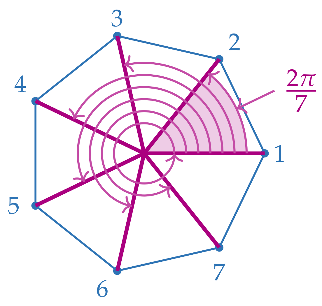
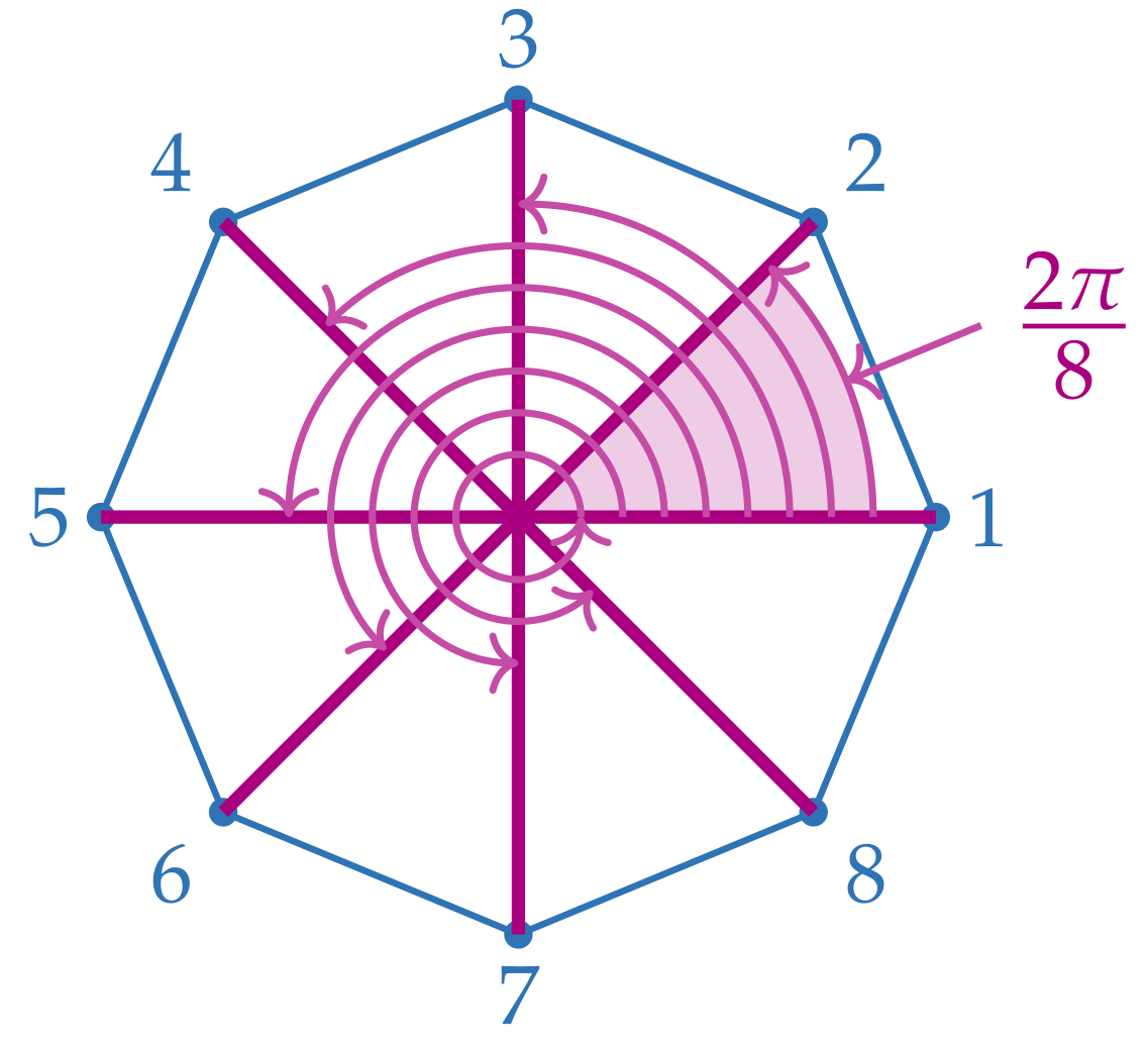
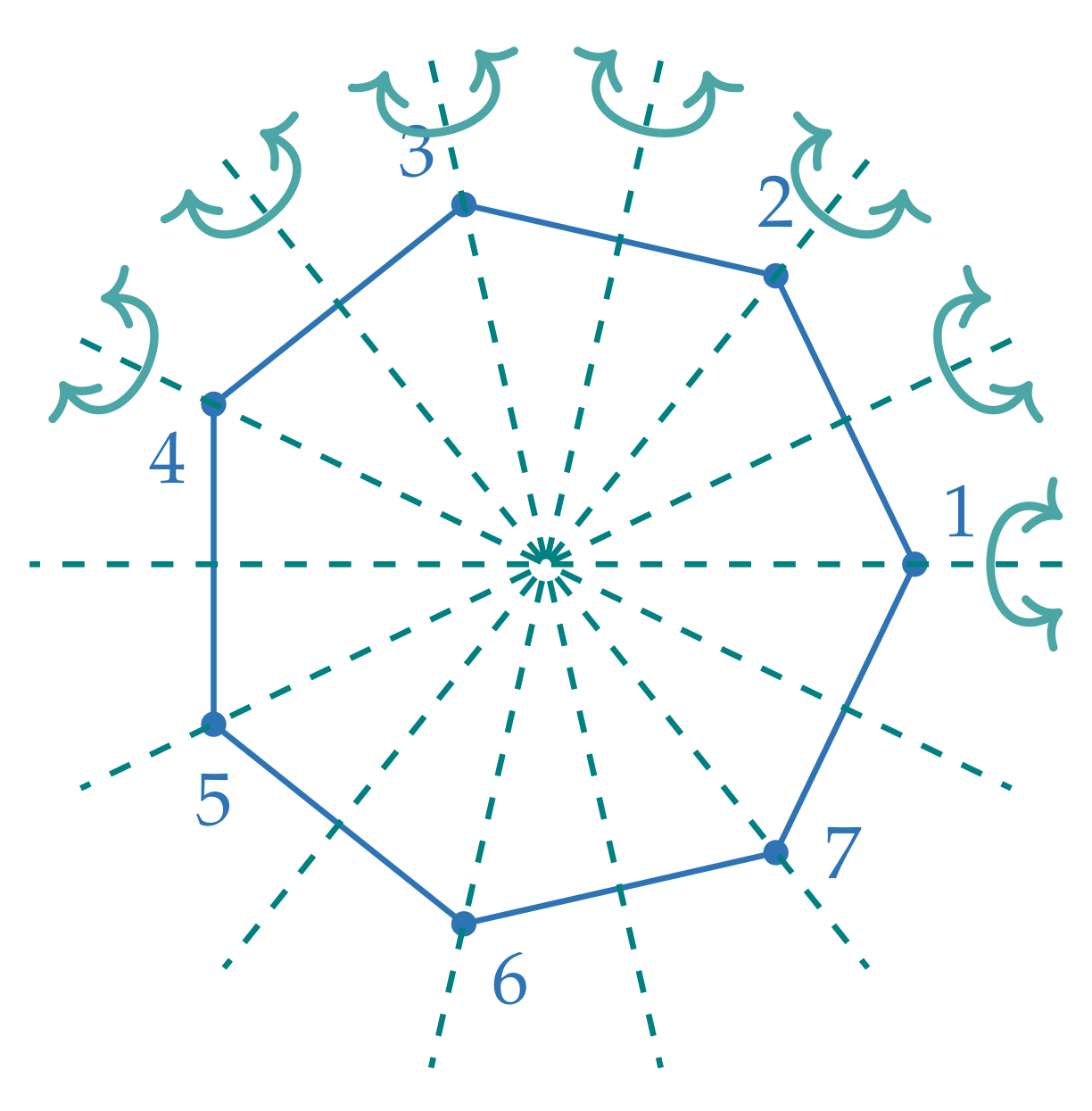
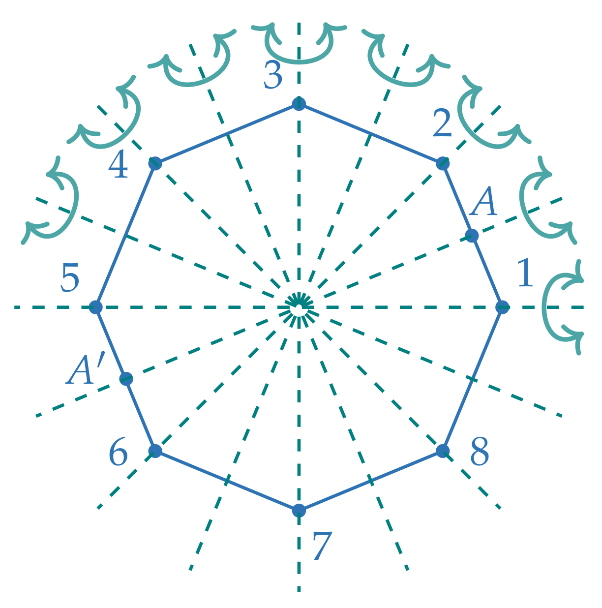
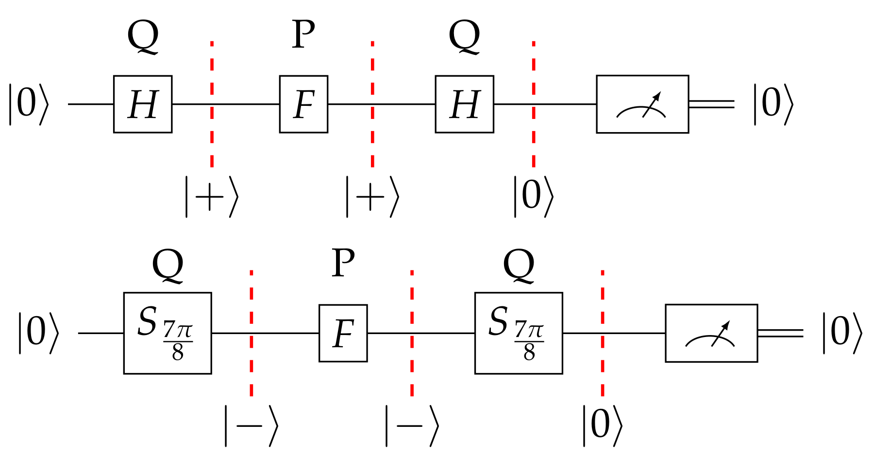
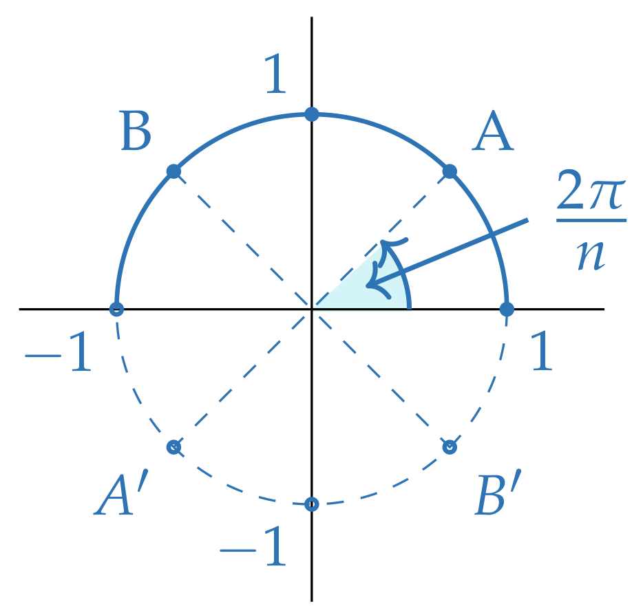
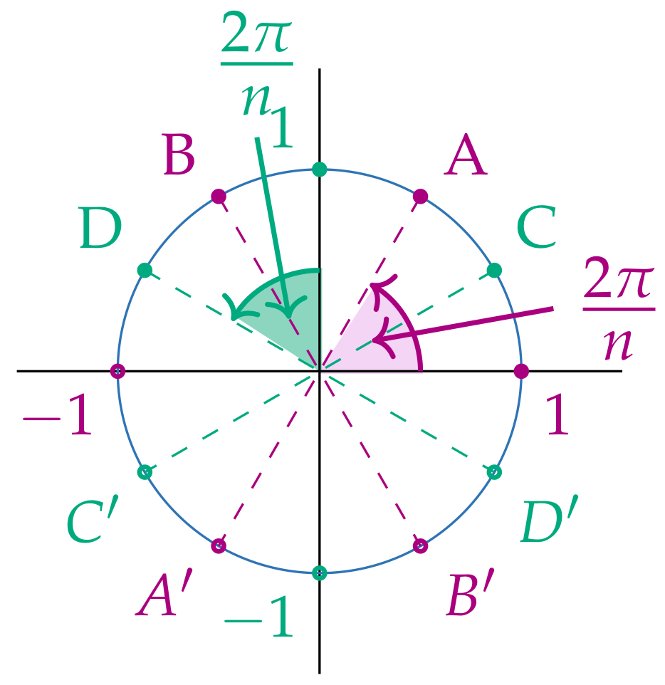
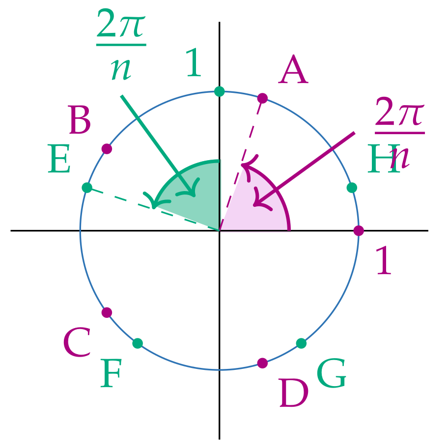
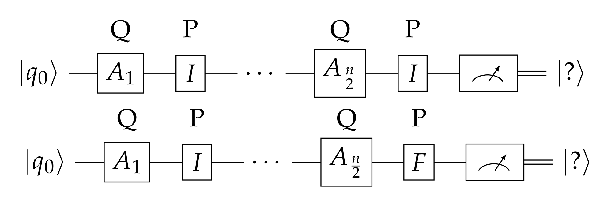
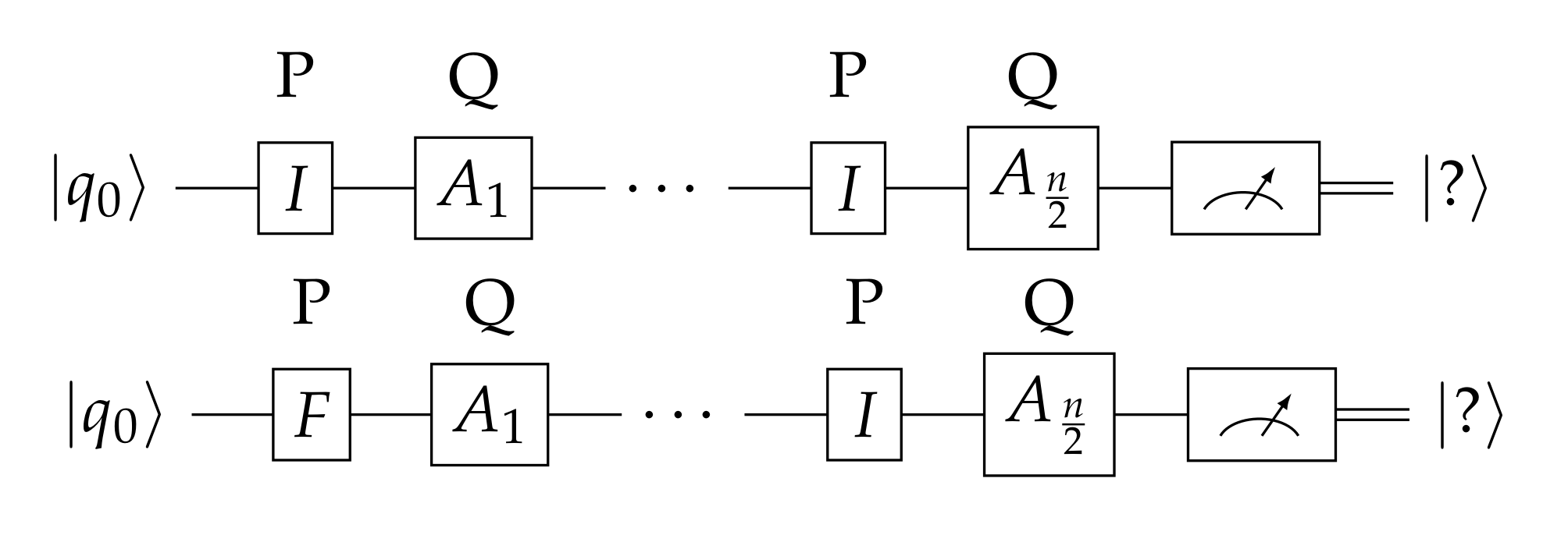
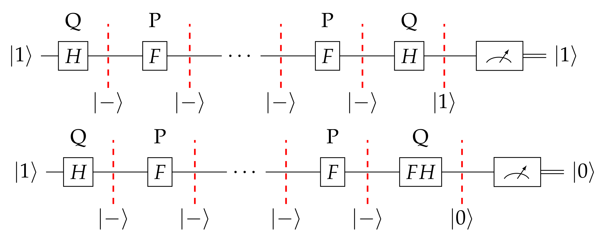
Table 1.
The two classes of winning and dominant strategies for Q in the original .
| The Evolution of the | ||||
|---|---|---|---|---|
| Initial State | Round 1 | Round 2 | Round 3 | |
Table 2.
In smaller dihedral groups, it is either impossible to play the , or, in the event that it is possible (such as in ), Q lacks a winning strategy. The abbreviation WS stands for winning strategy.
Table 2.
In smaller dihedral groups, it is either impossible to play the , or, in the event that it is possible (such as in ), Q lacks a winning strategy. The abbreviation WS stands for winning strategy.
| Ambient Group | Is PQG Playable | WS for Picard | WS for Q |
|---|---|---|---|
| No () | — | — | |
| Yes (classical coin tossing) | No | No | |
| No () | — | — | |
| No () | — | — | |
| No () | — | — |
Table 3.
The two classes of winning strategies for Q when the is played in a dihedral group and when the game is played in the largest possible group .
Table 3.
The two classes of winning strategies for Q when the is played in a dihedral group and when the game is played in the largest possible group .
| The Ambient Group is | ||||
|---|---|---|---|---|
| Initial State | Round 1 | Round 2 | Round 3 | |
| The Ambient Group is() | ||||
| Initial State | Round 1 | Round 2 | Round 3 | |
Publisher’s Note: MDPI stays neutral with regard to jurisdictional claims in published maps and institutional affiliations. |
© 2021 by the authors. Licensee MDPI, Basel, Switzerland. This article is an open access article distributed under the terms and conditions of the Creative Commons Attribution (CC BY) license (https://creativecommons.org/licenses/by/4.0/).
Share and Cite
MDPI and ACS Style
Andronikos, T.; Sirokofskich, A. The Connection between the PQ Penny Flip Game and the Dihedral Groups. Mathematics 2021, 9, 1115. https://0-doi-org.brum.beds.ac.uk/10.3390/math9101115
AMA Style
Andronikos T, Sirokofskich A. The Connection between the PQ Penny Flip Game and the Dihedral Groups. Mathematics. 2021; 9(10):1115. https://0-doi-org.brum.beds.ac.uk/10.3390/math9101115
Chicago/Turabian StyleAndronikos, Theodore, and Alla Sirokofskich. 2021. "The Connection between the PQ Penny Flip Game and the Dihedral Groups" Mathematics 9, no. 10: 1115. https://0-doi-org.brum.beds.ac.uk/10.3390/math9101115
Note that from the first issue of 2016, this journal uses article numbers instead of page numbers. See further details here.