Integral Models Based on Volterra Equations with Prehistory and Their Applications in Energy

Abstract

The paper addresses the application of Volterra integral equations of the first kind for modeling dynamic power systems. We study the problem of forecasting the commissioning of capacities of the electric power system, taking into account various hypotheses about the dynamics of equipment aging, and the known prehistory. The numerical results of the application of two models to the problem of the development of a large electric power system using the example of the Unified Energy System of Russia are presented. Theoretical results were formulated for a two-dimensional Volterra integral equation of the first kind with variable limits of integration. This class of equations arises when solving the actual problem of identifying variable characteristics of a nonlinear dynamic system of the “input-output” type.

1. Introduction

The main problems of the mathematical modeling of heat and power plants are associated, as a rule, with the identification [1] and diagnostics of the state [2] of technical objects. Depending on the types of models used, the following key directions can be chosen.

• Problems of calculating the statistical modes of power plants and their optimization [3]. Mathematical models for solving such problems are traditionally represented by systems of nonlinear algebraic equations, supplemented by a system of inequalities that ensure the feasibility of the parameter values. The methods for constructing such models are based mainly on the linearization of the original formulation of the problem.
• Problems of calculating dynamic characteristics and the analysis of transient processes. In terms of content, the mathematical tool takes into account the principles of hierarchical modeling of energy objects. In particular, in heat power engineering, separate formulations are considered for studying the dynamics of elements [4], sections of the steam-water path, and heat exchangers in general [5]. Nonlinear differential equations are the main research tool. At the same time, models of designed [6,7] and operating devices [8,9] are separated, the equipment state of which changes over time.
• Estimating the technical condition of heat and power equipment in order to analyze dynamic stability, prevent emergencies, replace obsolete equipment, and search for optimal technical parameters [10,11]. Mathematical models aimed at solving problems of this type are based on a detailed representation of electromechanical [12] and physicochemical processes [13].
• The problem of determining the optimal age structure of generating capacities, based on the analysis of the effectiveness of investment projects [14,15]. The age composition of the plants’ equipment is determined both by the volume of commissioning of new equipment and the scale of modernization and decommissioning of generating equipment. Such problems are often solved using linear programming methods [16].

The authors followed the following motivation when choosing the mathematical tools for research in this paper. Each of the problems listed above is described by that type of model, which is determined by the initial aim of modeling. This is not always convenient, since, in the course of modeling an object, you sometimes have to use different types of models. For example, first it is required to solve the problem of identifying the parameters of an object, and then, the problem of controlling the input or output signals. Furthermore, it would be nice to be able to model energy objects with different parameters using the same tool. The question arises about a universal approach that could be applied to various objects of heat and power engineering, depending on the meaning of the input and output parameters.

Models based on integral equations are one of these universal tools. The use of methods of integral equations for the analysis of dynamical systems developed intensively from the middle of the twentieth century. Then, this direction was supplanted in many applications by differential equations, being simpler and easier to study. The classical form of dynamic macroeconomic models [17] is based on the use of ordinary differential equations systems. This is inconvenient to a certain extent since actual dynamical systems can be described by non-smooth or even discontinuous functions. Moreover, the classical forms of presentation of dynamic models are poorly suited for describing the dynamics of delaying and completely refusing obsolete equipment. The description of dynamic models using systems of integral equations allows eliminating the indicated disadvantages. Furthermore, due to the greater compact notation and stability of the integration operation in comparison with the differentiation operation, integral representations have theoretical and applied advantages.

The analysis and application of the corresponding results show the relevance of the development of a mathematical apparatus based on high-speed integral models that describe well the dynamic properties of the systems studied and make it possible to provide a compromise between the modeling accuracy and the speed of computing algorithms. In this paper, we will consider the application of models based on non-classical Volterra integral equations to the modeling of the electric power system.

The purpose of our study is related to the problem of aging of the generating equipment of the electric power industry in Russia. The power of Russian power plants grew at the fastest rates during the 1980s. By now, all these capacities have worked out their resource. The commissioning of capacities has grown significantly only from the beginning of the 2010s. As a result, the average age of power plant equipment is 30–35 years, with the share of obsolete equipment being more than 50%.

The well-known models of the development of electric power systems (EPS) [18,19] do not describe aging processes; the analysis of the efficiency of equipment replacement is performed outside the framework of these models based on a general methodology for analyzing the effectiveness of investment projects [20].

Many works concerning the influence of equipment aging on the reliability of equipment operation at power facilities are known. In works [21,22,23], probabilistic methods are used to make decisions in the operation of obsolete equipment. The paper [24] proposes a method for applying ontologies to control the operation of aging equipment using online sensors to control mechanisms. All known mathematical models related to forecasting the development of the electric power industry are based on the use of linear programming and probabilistic methods.

The proposed dynamic model uses a fundamentally different mathematical apparatus based on non-classical Volterra integral equations. The main interest is the ability of the integral developmental model to describe the following factors:

• The dynamics of the commissioning of production facilities on the prehistory;
• The impact of scientific and technological progress;
• The mechanism of elements’ aging in dynamics due to the selection of several age groups;
• Decommissioning and replacement of obsolete equipment;
• The given dynamics of the available capacity in the future.

The developed model is used to analyze the long-term forecast of the commissioning of generating capacities with various strategies for dismantling obsolete capacities. Such an analysis is necessary for a qualitative analysis of the planning for the replacement of obsolete equipment within the framework of a large electric power system. A more detailed description of the generation structure was not used in our study. It should be noted that the model is universal and can be applied to analyze the development of a wide range of dynamical systems.

This paper is organized as follows. Section 2 consists of general information about the Volterra equation of the first kind with prehistory and the models based on it, including a relevant literature review. The application of the developed theory to problems in power engineering and the comparison of new results with those obtained earlier are considered in Section 3. Section 4 studies the specificity of two-dimensional integral equations of Volterra of the first kind with prehistory. The conclusion summarizes the main results and gives a perspective on future workings.

2. Integral Models Based on Volterra Equations of the First Kind

In 1977, V.M. Glushkov introduced a new class of integral models of developing systems [25]. The main distinguishing specialty of such models is the Volterra operators with variable lower limits of integration, reflecting the dynamics of replacing obsolete system elements with new ones. These models are based on the Volterra integral equation of the first kind

$$\underset{a\left(t\right)}{\overset{t}{{\displaystyle \int }}}K\left(t,s\right)x\left(s\right)ds=y\left(t\right), t\in \left[0,T\right],$$

(1)

where $x\left(t\right)$ is the number of new elements created in a time unit at time $t$; $K\left(t,s\right)$ is the labor productivity in the system; $a\left(t\right)$ is the time boundary of removing obsolete elements; and $y\left(t\right)$ is production of the external product at time $t$.

According to the terminology of [26], we will call such equations nonclassical to emphasize their difference from the standard Volterra equations of the first kind, for which only the upper limit of integration is variable. The specificity of (1) is largely determined by the values of the lower limits at the time of the origin of the system $a\left(0\right)$. The theory and numerical methods for solving Equation (1) for different initial conditions $a\left(0\right)<0$ and $a\left(0\right)=0$ have significant differences and were studied in detail in [26]. For the case of $a\left(0\right)<0$, it is necessary to specify the solution in prehistory $x\left(t\right)=x^0\left(t\right), t\in \left[a\left(0\right),0\right)$. It is this case that is characteristic of the integral models introduced by V.M. Glushkov and further developed in his works and the works of his followers [25,27,28,29]. For the existence, uniqueness, and continuity of the solution for (1) in $t\in \left[0,T\right]$, the conditions:

$$K_t^{\prime }\left(t,s\right)\in C_{∆}, ∆=\left\{t,s|a\left(t\right)\le s\le t, t\in \left[0,T\right]\right\};$$

$$K\left(t,t\right)\ne 0, t\in \left[0,T\right];$$

$$a^{\prime }\left(t\right)\ge 0, t\in \left[0,T\right];$$

$$t-a\left(t\right)>0, t\in \left[0,T\right];$$

$$y^{\prime }\left(t\right)\in C_{\left[0,T\right]};$$

$$x\left(t\right)=x^0\left(t\right), t\in \left[a\left(0\right),0\right)$$

must be satisfied, and the following two coordination conditions met:

$$y\left(0\right)=\underset{a\left(0\right)}{\overset{0}{{\displaystyle \int }}}K\left(0,s\right)x^0\left(s\right)ds;$$

$$y^{\prime }\left(0\right)=K\left(0,0\right)x^0\left(0\right)-a^{\prime }\left(0\right)K\left(0,a\left(0\right)\right)x^0\left(a\left(0\right)\right)+\underset{a\left(0\right)}{\overset{0}{{\displaystyle \int }}}{K}_t^{\prime }\left(0,s\right)x^0\left(s\right)ds.$$

The corresponding theorem and its proof are given in [26] (p. 60).

Since (1) has a solution in an analytical form only in special cases, numerical methods are used to solve it. Note that the application of the quadrature methods developed for the classical Volterra integral equations in solving (1) in case $a\left(0\right)<0$ leads to a loss of the order of convergence in the grid step. This is due to the appearance of an error in the approximation of the integral by quadrature in prehistory. Monograph [26] proposes modifications of quadrature methods to avoid this drawback.

The application of the apparatus of integral models of the Glushkov type for modeling EPS development began in the middle of the 1980s [30,31]. At the same time, the following notations were used to describe the EPS: $x\left(t\right)$ for $t\in \left[0,T\right]$ is the required total (for EPS) commissioning of electric capacities (MW); the kernel $K\left(t,s\right)$ is an efficiency coefficient of $x\left(t\right)$ at the moment $t$ (describes the process of physical aging of the equipment); $t-a\left(t\right)$ is the lifetime (year) of the oldest electric capacities in the EPS at the moment $t$; $x^0\left(t\right)$ is the known commissioning of electric capacities (MW) in prehistory $\left[\mathrm{a}\left(0\right),0\right)$. The right-hand side of Equation (1) $y\left(t\right)$ determines the total available capacity of the EPS (MW) at moment $t$, taking into account the decommissioning of the capacities after their lifetime.

In following works [32,33,34,35,36], mathematical models of the development of generating capacities of EPS were considered with different degrees of aggregation by power plant types. There are estimated models (analysis of the consequences of a given strategy for renewing capacities), optimization ones (optimization of the capacities lifetime), and models that describe the processes of extending the lifetime of generating equipment (modernization). The model of EPS development based on integro-algebraic equations with variable limits of integration is presented in [37].

In [38,39], in connection with the study of the Volterra equation of the first kind with a discontinuous kernel, the integral equation

$${\displaystyle \sum }_{i=1}^n\underset{a_i\left(t\right)}{\overset{a_{i-1}\left(t\right)}{{\displaystyle \int }}}{K}_i\left(t,s\right)x\left(s\right)ds=y\left(t\right), t\in \left[0,T\right],$$

(2)

was considered, where $a_i\left(0\right)=0, i=\overline{0,n};$ $a_0\left(t\right)\equiv t, a_n\left(t\right)\equiv 0$. This equation can be considered a generalization of Equation (1) ((2) turns into (1) for $n=1$).

In work [40], A.S. Apartsyn proposed Equation (2) to be taken as the basis for constructing an integral model for the development of EPS, taking into account the aging of its elements. Such models make it possible to describe in detail the technical and economic parameters of the generating equipment of EPS power plants, taking into account its age structure. For this, all generating equipment is divided into certain age groups with different technical and economic parameters of the equipment functioning, reflecting the aging processes.

Equation (2) was studied in [41,42]. In [42], sufficient Hadamard correctness conditions of the problem (2) on the pair $\left(C_{\left[0,t\right]},C{°}_{\left[0,t\right]}^{\left(1\right)}\right)$ are given. Here, by $C{°}_{\left[0,t\right]}^{\left(1\right)}$ we mean a space of functions $y\left(t\right)$ continuously differentiable on $\left[0,T\right]$ with the condition $y\left(0\right)=0$.

Three types of models describing different assumptions about the mechanisms of system elements aging were proposed in [40]. This paper discusses examples of applying two of them to modeling long-term strategies for the development of a large EPS.

2.1. Model 1

In the model of the first type [40], it is assumed that the functions of transition from one age group to another have the form $a_i\left(t\right)=t-T_i$, $i=\overline{0,n},T_0=0$; the efficiency coefficient is a constant value within one age group, i.e., $K_i\left(t,s\right)\equiv {\beta }_i$, at which $1\equiv {\beta }_1\ge {\beta }_2\ge \dots \ge {\beta }_n\ge 0$. Moreover, ${\beta }_n\equiv 0$ means the decommissioning of capacities whose age exceeds the age limit $T_{n-1}$.

Four age groups are identified in the EPS development model: young (new) capacities, middle-aged and older capacities with deteriorated technical and economic parameters due to aging, and even older capacities decommissioned, for which ${\beta }_4\equiv 0$.

According to (2), for such age groups, we have the following equation:

$$\underset{t-T_1}{\overset{t}{{\displaystyle \int }}}x\left(s\right)ds+{\beta }_2\underset{t-T_2}{\overset{t-T_1}{{\displaystyle \int }}}x\left(s\right)ds+{\beta }_3\underset{t-T_3}{\overset{t-T_2}{{\displaystyle \int }}}x\left(s\right)ds=y\left(t\right), t\in \left[t_0,T\right],$$

(3)

where $t_0$ is the moment of the beginning of the forecast, which may not coincide with the beginning of the system origin. A theorem was proven on the existence and uniqueness of a solution for (3) in the class of piecewise continuous functions, and an algorithm was given for determining the discontinuity points of a solution on any finite segment [40].

Mathematical models of the development of generating capacities of EPS based on the model (3) at $t_0>T_3$ were considered with different degrees of aggregation by power plant types. The problem of choosing the optimal integrated strategy for the decommissioning of obsolete generating equipment using optimization models was investigated. In addition, the influence of economic indices on the solution of the optimal control problem was studied [43,44,45].

2.2. Model 2

The difference of this type of model compared to the previous one is that continuous functions within the limits of integration $a_i\left(t\right)$ satisfy the conditions $t\equiv a_0\left(t\right)>a_1\left(t\right)>\cdots >a_n\left(t\right)\equiv 0\forall t>0;$ $a_i\left(0\right)=0,i=\overline{1,n}$, $a_i^{\prime }\left(t\right)\ge 0$, $a_n^{\prime }\left(0\right)<\cdots <a_1^{\prime }\left(0\right)<1$.

Thus, the process of dividing its elements into groups with different efficiency indices begins from the moment when the system emerges.

Let, in the model of EPS development, $a_i\left(t\right)={\alpha }_{i}t$, $i=\overline{0,n}$, ${\alpha }_i$ is a constant value, $1\equiv {\alpha }_0>{\alpha }_1>\dots >{\alpha }_n\equiv 0$, efficiency coefficients $K_i\left(t,s\right)$ will still be constant, so (2) has the form

$$\underset{{\alpha }_{1}t}{\overset{t}{{\displaystyle \int }}}x\left(s\right)ds+{\displaystyle \sum }_{i=2}^n{\beta }_i\underset{{\alpha }_{i}t}{\overset{{\alpha }_{i-1}t}{{\displaystyle \int }}}x\left(s\right)ds=y\left(t\right), t\in \left[0,T\right].$$

(4)

It was shown that Equation (4) is well-posed in the sense of Hadamard on the pair $\left(C_{\left[0,t\right]},C{°}_{\left[0,t\right]}^{\left(1\right)}\right)$ under the following condition [40]:

$${\displaystyle \sum }_{i=2}^n\left|{\beta }_{i-1}-{\beta }_i\right|{\alpha }_{i-1}<1$$

Thus, both models describe the functioning of a system consisting of $n$ age groups. In the model of the first type, it is assumed that from the beginning of the system origin until the moment $T_1$, all elements function with maximum efficiency ${\beta }_1$ and belong to the same age group, the rest of the groups are empty. At the moment $T_1$, the next age group appears with efficiency ${\beta }_2$ $\mathrm{and}\mathrm{so}\mathrm{on}\mathrm{up}\mathrm{to}$ $T_{n-1}$. Elements older than $T_{n-1}$ are retired.

In the model of the second type, at the moment of the system origin, all groups appear at the same time. At the moment $t$, those elements whose age has exceeded the value ${\alpha }_{i}t$ move from group $i$ to group $i+1$. The retirement of capacities occurs when the capacity moves to group $n$, the efficiency of which is equal to 0.

The next section is devoted to using the developed theory for applications in power engineering.

3. Applying Integral Models for Modeling Long-Term Strategy of Electric Power Systems

The purpose of this section is to use two approaches to describing the aging of elements in a developing EPS model to study the adequacy of the model to actual processes and to develop various strategies for commissioning EPS equipment.

3.1. Problem of Determining Long-Term Strategies Based on Model 1

The problem of determining the long-term development strategies of the EPS of Russia based on the development model (3) was considered in [40]. This is the problem of determining the dynamics of commissioning of capacities $x\left(t\right)$, which provide a given growth rate of available capacity $y\left(t\right)$. It was assumed that the beginning of modeling coincides with the moment of the system emergence. For the EPS of Russia, 1950 was taken as zero (the moment of the system emergence). It is one of the post-war years with a sharp increase in the commissioning of capacities. The parameters $T_1=30$, $T_2=50$, $T_3=60$, and $T=100$ (corresponding to 2050) were taken to describe age boundaries, ${\beta }_1=1$, ${\beta }_2=0.97$, and ${\beta }_3=0.9$. In this model, all capacities belong to the same age group in the interval $\left[0,T_1\right]$. The second age group is formed at the moment $T_1$. The third and the fourth age groups are formed at the moments $T_2$ and $T_3$, correspondingly.

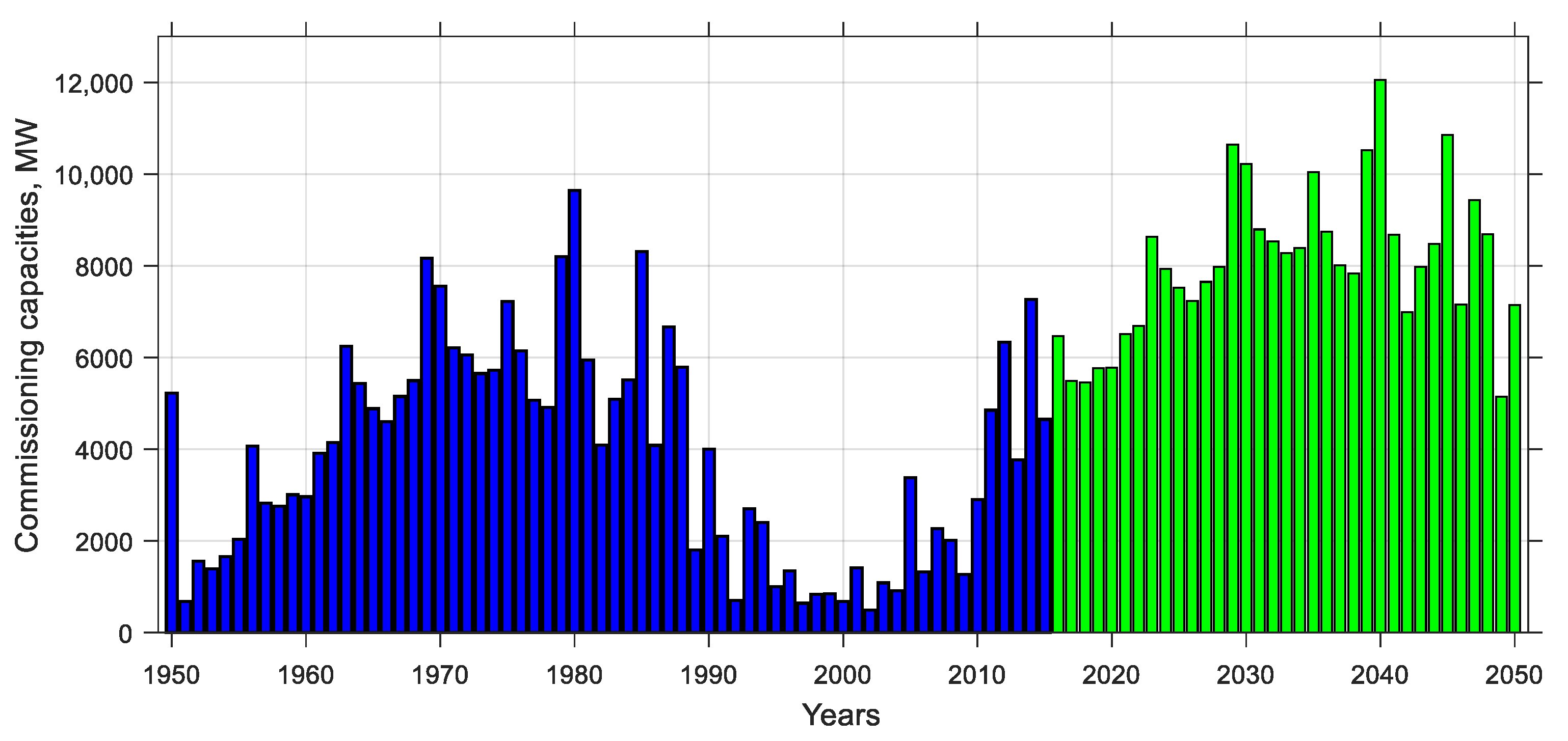
Let us give an example of using model (3) with the use of actual data on the commissioning of capacities in prehistory. The value $t_0=2016$ is taken for the beginning of the forecasting period. The dynamics of commissioning capacity is known in prehistory (from 1950 to 2015) [46]: $x\left(t\right)=x^0\left(t\right), t\in \left[1950, 2015\right]$. The growth of the right-hand side $y\left(t\right)$ is 1% per year from the level of 2015. Using (3), the dynamics of commissioning of new capacities are determined, starting from 2016 and up to 2050 inclusive. The integrals in (3) were approximated using the right rectangles method with a step $h=1$ (year). Figure 1 shows the solution to the forecasting problem. The dynamics of commissioning capacities in prehistory is marked in blue, the forecasted values of commissioning capacities in green.

If we consider the vector case when the equipment of power plants is divided into several types (for example, fossil fuel-fired plants—TPPs, nuclear-fueled plants—NPPs, and hydroelectric power plants—HPPs), then the mathematical model of EPS development is a system of equations:

$${\displaystyle \sum }_{i=1}^3\left({\beta }_{i1}\underset{t-T_{i1}\left(t\right)}{\overset{t}{{\displaystyle \int }}}{x}_i\left(s\right)ds+{\beta }_{i2}\underset{t-T_{i2}\left(t\right)}{\overset{t-T_{i1}\left(t\right)}{{\displaystyle \int }}}{x}_i\left(s\right)ds+{\beta }_{i3}\underset{t-T_{i3}\left(t\right)}{\overset{t-T_{i2}\left(t\right)}{{\displaystyle \int }}}{x}_i\left(s\right)ds\right)=y\left(t\right), t\in \left[t_0,T\right].$$

(5)

$$\underset{t-T_{13}\left(t\right)}{\overset{t}{{\displaystyle \int }}}{x}_1\left(s\right)ds={\gamma }_1\left(t\right)\left(\underset{t-T_{13}\left(t\right)}{\overset{t}{{\displaystyle \int }}}{x}_1\left(s\right)ds+\underset{t-T_{23}\left(t\right)}{\overset{t}{{\displaystyle \int }}}{x}_2\left(s\right)ds+\underset{t-T_{33}\left(t\right)}{\overset{t}{{\displaystyle \int }}}{x}_3\left(s\right)ds\right),$$

(6)

$$\underset{t-T_{33}\left(t\right)}{\overset{t}{{\displaystyle \int }}}{x}_3\left(s\right)ds={\gamma }_3\left(t\right)\left(\underset{t-T_{13}\left(t\right)}{\overset{t}{{\displaystyle \int }}}{x}_1\left(s\right)ds+\underset{t-T_{23}\left(t\right)}{\overset{t}{{\displaystyle \int }}}{x}_2\left(s\right)ds+\underset{t-T_{33}\left(t\right)}{\overset{t}{{\displaystyle \int }}}{x}_3\left(s\right)ds\right),$$

(7)

$$x_i\left(t\right)=x_i^0\left(t\right), t\in \left[0,t_0\right),$$

(8)

$$x_i\left(t\right)\ge 0, t\in \left[t_0,T\right].$$

(9)

Here, the index “1” for the commissioning capacities corresponds to TPP, “2”—NPP, “3”—HPP; ${\beta }_{ij}$ is the efficiency coefficient for equipment of age group $j$ on a power plant of type $i$; $y\left(t\right)$ is the total available capacity of the electric power system forecasted by experts; $T_{ij}\left(t\right)$ is the upper boundary of the age group $j$ for a power plant of type $i$, $i,j=\overline{1,3}$, $0<T_{i1}\left(t\right)<T_{i2}\left(t\right)<T_{i3}\left(t\right)$; $T_{i3}\left(t\right)$ is the lifetime of the equipment of type $i$ (the age of the oldest equipment of type $i$ still in use at the moment $t$); $x_i^0\left(t\right)$ are the known commissioning of electric capacities of type $i$ in prehistory; ${\gamma }_1\left(t\right)$ and ${\gamma }_3\left(t\right)$ are the proportions of TPP and HPP capacities, correspondingly, in the total composition of generating equipment.

The numerical scheme constructed using the quadrature of the right rectangles to approximate the integrals in (5)–(9) involves solving a system of linear algebraic equations at each time step. Moreover, it is important that the nonnegativity condition for the commissioning capacities (9) be satisfied. If negative values are obtained, we replace them with zeros (we do not input anything this year), that is, in fact, in (5) we have inequality instead of equality. Figure 2 shows the solution of the forecasting problem for the vector case. The forecasted values of commissioning capacities (from 2016 to 2050) are shown by narrow bars. As you can see, the annual total value of the commissioning capacities coincides with the scalar case, which confirms the correct operation of the model.

The problem of optimizing the lifetime of TPP and NPP equipment was considered in [44] on the basis of the model (5)–(9). The problem is to find such dynamics of the commissioning of capacities, which would deliver a minimum of total costs for the commissioning of new and operation of generating capacities for a given demand for electricity. A detailed description of the numerical solution of the optimization problem and the calculation results for actual data for the Unified Energy System of Russia are given in [44].

3.2. Problem of Determining Long-Term Strategies Based on Model 2

The problem of identifying the parameters ${\alpha }_i$, ${\beta }_i$ in model (4) is an independent complex problem. Therefore, in this work, we will focus on the case of two age groups:

$$\underset{{\alpha }_{1}t}{\overset{t}{{\displaystyle \int }}}x\left(s\right)ds+\beta \underset{{\alpha }_{2}t}{\overset{{\alpha }_{1}t}{{\displaystyle \int }}}x\left(s\right)ds=y\left(t\right), t\in \left[t_0,T\right].$$

Using the known data of commissioning of capacities $x\left(t\right)$ and available capacity $y\left(t\right)$ in prehistory from 1950 to 2015, the parameters ${\alpha }_1=0.35$, ${\alpha }_2=0.08, \mathrm{and} \beta =0.94$ were selected in an expert way. The beginning of the forecasting period is also $t_0=2016$.

In this model, at the time of the system origin, three groups of capacities are formed at once. The efficiency coefficients in the groups are 1, 0.94, and 0, correspondingly. Setting the growth of the right-hand side $y\left(t\right)$ 1% per year in $\left[2016,2050\right]$ and taking into account the dynamics of commissioning capacities from 1950 to 2015 [46] (marked in Figure 3 in blue), using the numerical method, we obtain the dynamics of commissioning of new capacities in the forecasting period from 2016 to 2050 inclusive (marked in Figure 3 in green).

As for the numerical solution of (4), it should be noted that using quadrature methods developed for the numerical solution of the classical Volterra equations, concerning Equation (4) can lead to the fact that just at the first grid node an equation with $n$ unknowns can arise, where $n$ is the number age groups in the model. The reason for this is the possible discrepancy between the values of the integration limits $a_i\left(t_j\right)$ and the nodes of the uniform grid $t_j=jh, j=\overline{1,N, } Nh=T$. A modification of the left rectangles method was proposed [47], based on the transformation of the original equation to an equivalent one, in which only the upper limits of integration are variables. The constructed numerical scheme has the first order of convergence, as in the classical case. Figure 3 shows the results obtained by the modified method of left rectangles with a step $h=1$, which provide a given growth rate of the available capacity $y\left(t\right).$

Further setting various hypotheses about the growth rates of $y\left(t\right)$ for the forecasting period, it is possible to obtain the corresponding options for the commissioning of capacities that provide a given growth dynamics of the available capacity.

Comparison of the results of applying model 1 and model 2 (Figure 1 and Figure 3) shows the obvious influence of the behavior of the dynamics of commissioning of capacities in prehistory on the behavior of the solution in the forecasting period. In the first case, we have a solution with noticeable jumps, and model 2 gives a smoother solution, which is more consistent with the description of the evolutionary process.

Thus, the constructed models take into account the inertia of the EPS development in different ways and can be used as suitable methods for modeling the processes of replacing obsolete equipment in a production system. However, the decision on the preference of the model must be made by electric power specialists.

In further studies, it is assumed that model 2 will be used for more complex cases (when the number of age groups is more than 2 and the plants are divided by fuel type).

4. On Two-Dimensional Volterra Equations of the First Kind with Prehistory

Further development of the work is associated with applying multidimensional Volterra integral equations of the first kind with prehistory. To illustrate the complexity of such a transition, let us consider the specifics of two-dimensional Volterra integral equations of the first kind with prehistory.

Unlike the one-dimensional Volterra equation of the first kind (1), for which the theory and numerical methods are quite well developed, a developed theory of multidimensional equations with prehistory, apparently, does not yet exist. Fundamental results related to $n$-dimensional equations with variable upper and lower limits of integration

$$s_p=t-{\displaystyle \sum }_{i=0}^p{\omega }_i,$$

(10)

where ${\omega }_0=0$, $t, {\omega }_p\in {\pi }_p=\left\{t, {\omega }_0,\dots ,{\omega }_p: 0\le {\displaystyle \sum }_{j=0}^p{\omega }_j\le t\le T, {\omega }_j\ge 0\right\}, p=\overline{0,n-1}$, are presented in the monograph [26]. In it, the main focus is placed on the situation when the integrand $\phi$ does not explicitly depend on the time $t$. The adaptation of the results presented in [26] to equations in which φ varies with time, so that

$$s_{p+1}={\displaystyle \sum }_{i=0}^{p+1}{\omega }_i,$$

$$t, {\omega }_{p+1}\in {\pi }_{p+1}=\left\{t, {\omega }_0,\dots ,{\omega }_{p+1}: 0\le {\displaystyle \sum }_{j=0}^{p+1}{\omega }_j\le t\le T, {\omega }_j\ge 0\right\}, p=\overline{0,n-1},$$

takes place instead of (10), is given in [48].

To represent the difficulties arising in the transition from (10), where $n\ge 2$, to an equation with limits of integration $s_p, s_p-h$, such that

$$t,{\omega }_p\in {\widehat{\pi }}_p=\left\{t, {\omega }_1,\dots ,{\omega }_p:h\le t\le T, {\displaystyle \sum }_{j=1}^p{\omega }_j\le t-h, {\omega }_j\ge 0\right\}, h>0, p=\overline{1,n-1},$$

(11)

we recall the known facts for limits of the form (10) in the most important case for applications $n=2$. Consider the situation when the integrand is non-symmetric for the variables ${\lambda }_1,{\lambda }_2$ [26] (p. 151):

$$\begin{array}{c}\underset{0}{\overset{s_0}{{\displaystyle \int }}}d{\lambda }_1\underset{s_1}{\overset{s_0}{{\displaystyle \int }}}\phi \left({\lambda }_1,{\lambda }_2\right)d{\lambda }_2=f_1\left(s_0,s_1\right),\\ \underset{s_1}{\overset{s_0}{{\displaystyle \int }}}d{\lambda }_1\underset{0}{\overset{s_0}{{\displaystyle \int }}}\phi \left({\lambda }_1,{\lambda }_2\right)d{\lambda }_2=f_2\left(s_0,s_1\right), \end{array}$$

(12)

$s_0=t, s_1=t-{\omega }_1;t, {\omega }_1\in {\pi }_2; s_0,s_1\in {\mathsf{\Pi }}_2^{\left(1\right)}=\left\{{\rm M}\left(p,q\right):0\le s_1\le q\le p\le s_0\le T\right\}$, where ${\rm M}\left(p,q\right)$ is a point of the plane with Cartesian coordinates $\left(p,q\right)$.

Let it take place

$${\left(f_i\right)}_{s_0{s}_1}^{″}\in C_{{\mathsf{\Pi }}_2^{\left(1\right)}}, i=1, 2;$$

(13)

$$f_i\left(s,s\right)=0, f_1\left(s,0\right)=f_2\left(s,0\right)\left(=f\left(s,0\right)\right), s\in \left[0,T\right];$$

(14)

$$\frac{1}{2}\left(f_1\left(s_0,s_1\right)+f_2\left(s_0,s_1\right)\right)=\frac{1}{2}\left(f_1\left(s_1,s_0\right)+f_2\left(s_1,s_0\right)\right)+f\left(s_0,0\right)-f\left(s_1,0\right);$$

(15)

$${{\left(f_1\right)}_{s_0{s}_1}^{″}|}_{s_0=s_1=s}={{\left(f_2\right)}_{s_0{s}_1}^{″}|}_{s_0=s_1=s}.$$

(16)

Then Equations (13)–(16) are necessary and sufficient conditions for the existence of a solution for Equation (12)

$$\phi \left(s_0,s_1\right)=-{\left(f_1\right)}_{s_0{s}_1}^{″}, \phi \left(s_1,s_0\right)=-{\left(f_2\right)}_{s_0{s}_1}^{″}$$

in the class $C_{{\mathsf{\Pi }}_2}$, ${\mathsf{\Pi }}_2=\left\{{\rm M}\left(p,q\right):0\le s_1\le p,q\le s_0\le T\right\}$. Moreover, the satisfaction of the condition

$${\left[{\left(f_1\right)}_{s_1}^{\prime }+{\left(f_2\right)}_{s_1}^{\prime }\right]|}_{s_0=s_1=s}=-{{\left(f_1\right)}_{s_0}^{\prime }|}_{\begin{array}{c}{s}_0=s\\ s_1=0\end{array}}\left(=-{{\left(f_2\right)}_{s_0}^{\prime }|}_{\begin{array}{c}{s}_0=s\\ s_1=0\end{array}}\right)$$

(17)

in addition to (13)–(16) ensures the uniqueness of the solution for (12) in the class $C_{{\mathsf{\Pi }}_2}$. Let us focus on an important fact. The integral operators in (12) contain integration domains lying in both ${\mathsf{\Pi }}_2^{\left(1\right)}$ and ${\mathsf{\Pi }}_2^{\left(2\right)}=\left\{{\rm M}\left(p,q\right):0\le s_1\le p\le q\le s_0\le T\right\}$, since ${\mathsf{\Pi }}_2={\mathsf{\Pi }}_2^{\left(1\right)}{\displaystyle \cup }{\mathsf{\Pi }}_2^{\left(2\right)}$.

The purpose of this section is to obtain conditions of the type (13)–(16), (17) that ensure the existence and uniqueness of the solution $\overline{\phi }$ of the pair equation

$$\begin{array}{c}\underset{t-h}{\overset{t}{{\displaystyle \int }}}d{\lambda }_1\underset{t-\nu -h}{\overset{t-\nu }{{\displaystyle \int }}}\phi \left({\lambda }_1,{\lambda }_2\right)d{\lambda }_2=g_1\left(t,\nu \right),\\ \underset{t-\nu -h}{\overset{t-\nu }{{\displaystyle \int }}}d{\lambda }_1\underset{t-h}{\overset{t}{{\displaystyle \int }}}\phi \left({\lambda }_1,{\lambda }_2\right)d{\lambda }_2=g_2\left(t,\nu \right), \end{array}$$

(18)

$h\le t\le T$, $\nu \le t-h$, in the class $C_{\left[h,T\right]}$ with known

$$\overline{\phi }\left({\lambda }_1,\lambda \right)={\phi }^{\left(0\right)}\left({\lambda }_1,\lambda \right), \overline{\phi }\left(\lambda ,{\lambda }_2\right)={\phi }^{\left(0\right)}\left(\lambda ,{\lambda }_2\right),$$

(19)

$${\lambda }_1,{\lambda }_2\in \left[0,h\right), \lambda \in \left[0,T\right].$$

(20)

In (18), we denote ${\omega }_1$ from (11) by $\nu$ for simplicity. The fundamental point concerns the determination of the desired solution $\overline{\phi }$ at the initial point $t_0$ of the segment $\left[h,T\right]$. To prevent overdetermination of problem (18) and (19), prehistory (20) does not include the boundary $t_0=h$. Moreover, if in case (12) the continuity of $\overline{\phi }$ follows from (13)–(16), then, as applied to (18)–(20), additional coordination conditions are required.

As shown in [49], the solution to the problem (18)–(20) is defined by the formulas

$$\begin{array}{c}\overline{\phi }\left(t,t-\nu \right)\equiv {\displaystyle {\displaystyle \sum }_{i=1}^{N+1}}{\phi }^{\left(i\right)}\left(t,t-\nu \right)=\\ ={{\displaystyle {\displaystyle \sum }_{i=1}^{N+1}}{\mathcal{D}}_2{g}_1|}_{N\in {∆}_i}+{\displaystyle {\displaystyle \sum }_{i=1}^{N+1}}\left({\phi }^{\left(i-1\right)}\left(t,t-\nu -h\right)+{\phi }^{\left(i-1\right)}\left(t-h,t-\nu \right)-{\phi }^{\left(i-1\right)}\left(t-h,t-\nu -h\right)\right),\end{array}$$

(21)

$$\begin{array}{c} \\ \begin{array}{c}\overline{\phi }\left(t-\nu ,t\right)\equiv {\displaystyle {\displaystyle \sum }_{i=1}^{N+1}}{\phi }^{\left(i\right)}\left(t-\nu , t\right)=\\ ={{\displaystyle {\displaystyle \sum }_{i=1}^{N+1}}{\mathcal{D}}_2{g}_2|}_{N\in {∆}_i}+{\displaystyle {\displaystyle \sum }_{i=1}^{N+1}}\left({\phi }^{\left(i-1\right)}\left(t-\nu -h,t\right)+{\phi }^{\left(i-1\right)}\left(t-\nu ,t-h\right)-{\phi }^{\left(i-1\right)}\left(t-\nu -h,t-h\right)\right),\end{array}\end{array}$$

(22)

where

$$\begin{array}{c}{\mathcal{D}}_2{g}_j\left(t,\nu \right)=-\left({\left(g_j\right)}_{t\nu }^{″}+{\left(g_j\right)}_{{\nu }^2}^{″}\right), j=1, 2,\\ N=\frac{T}{h}, {\mathsf{\Delta }}_k=\left\{t,\nu : \nu +h\le t, kh\le t\le \left(k+1\right)h\right\}, k=\overline{1,N},\\ {\mathsf{\Delta }}_{N+1}=\left\{t,\nu : \nu +h\le t, Nh\le t\le T\right\}.\end{array}$$

(23)

In (21) and (22), $N\left(t,\nu \right)$ denotes a point on the plane with Cartesian coordinates $\left(t,\nu \right)$; ${\phi }^{\left(i-1\right)}\left({\rm M}\right)$ and ${\phi }^{\left(i-1\right)}\left(\overline{{\rm M}}\right)$ is a solution to Equation (18) for ${\rm M}\left(p,q\right), t-\nu \le q\le p\le t,$ and $\overline{{\rm M}}\left(p,q\right), t-\nu \le p\le q\le t,$ from the subdomains ${\mathsf{\Omega }}_{i-1}\left(N\left(t,\nu \right)\right)$, in which the coordinates $N\left(t,\nu \right)$ correspond to ${\mathsf{\Delta }}_k, k=\overline{0,N,}$ with the corresponding index $i-1$, while ${\mathsf{\Delta }}_0$ is prehistory:

$${\mathsf{\Delta }}_0=\left\{t,\nu : D_1{\displaystyle \cup }{D}_2, \nu \ge 0\right\}, D_1=\left\{t,\nu : \nu \le t, 0\le t <h, h >0\right\},$$

$$D_2=\left\{t,\nu : t-h<\nu \le t, h\le t\le T, h>0\right\}.$$

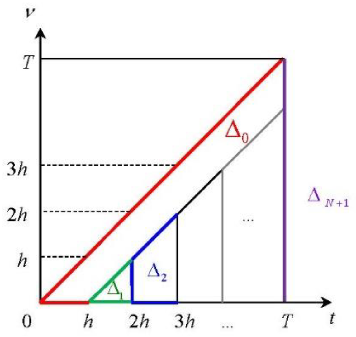
An illustration of the location of the ${\mathsf{\Delta }}_k$ for $k=0, 1, 2,\dots ,N+1$ is shown in Figure 4.

The method for obtaining (21) and (22) is described in detail in [49] and is based on the classical method of steps [50], which has proven itself in solving one-dimensional Volterra equations of the first kind with prehistory [26]. For convenience, we rewrite (18) in operator form, using the change of variables (11): $s_0=t$, $s_1=t-\nu$, so that, taking into account

$$\begin{array}{c}{V}_{1,2}\phi \equiv \underset{s_0-h}{\overset{s_0}{{\displaystyle \int }}}d{\lambda }_1\underset{s_1-h}{\overset{s_1}{{\displaystyle \int }}}\phi \left({\lambda }_1,{\lambda }_2\right)d{\lambda }_2,\\ V_{2,1}\phi \equiv \underset{s_{1-h}}{\overset{s_1}{{\displaystyle \int }}}d{\lambda }_1\underset{s_0-h}{\overset{s_0}{{\displaystyle \int }}}\phi \left({\lambda }_1,{\lambda }_2\right)d{\lambda }_2, \end{array}$$

instead of (18), setting $g_i\left(s_0,s_0-s_1\right)=y_i\left(s_0,s_1\right), i=1,2$, we have

$$V_{1,2}\phi =y_1\left(s_0,s_1\right), V_{2,1}\phi =y_2\left(s_0,s_1\right),$$

(24)

$$s_0,s_1\in {\mathsf{\Omega }}^{\left(1\right)}=\underset{k=1}{\overset{N+1}{{\displaystyle \cup }}}{\mathsf{\Omega }}_k^{\left(1\right)}\left(N\left(s_0,s_0-s_1\right)\right),$$

where ${\mathsf{\Omega }}_k^{\left(1\right)}\left(N\left(s_0,s_0-s_1\right)\right)=\left\{{\rm M}\left(p,q\right):s_1\le q\le p\le s_0,N\left(s_0,s_0-s_1\right)\in {∆}_k\right\}$, ${∆}_k\left(k=\overline{1,N+1}\right)$ are given by (23). Equations (21) and (22) in the new notation can be rewritten as:

$$\begin{array}{c}\overline{\phi }\left({\rm M}\right)={{\displaystyle {\displaystyle \sum }_{i=1}^{N+1}}{\left(y_1\right)}_{s_0{s}_1}^{″}|}_{N\in {∆}_i}+\\ +{\displaystyle {\displaystyle \sum }_{i=1}^{N+1}}\left({\phi }^{\left(i-1\right)}\left(s_0,s_1-h\right)+{\phi }^{\left(i-1\right)}\left(s_0-h,s_1\right)-{\phi }^{\left(i-1\right)}\left(s_0-h,s_1-h\right)\right), {\rm M}\in {\mathsf{\Omega }}^{\left(1\right)},\end{array}$$

(25)

$$\begin{array}{c}\overline{\phi }\left(\overline{{\rm M}}\right)={{\displaystyle {\displaystyle \sum }_{i=1}^{N+1}}{\left(y_2\right)}_{s_0{s}_1}^{″}|}_{N\in {∆}_i}+\\ +{\displaystyle {\displaystyle \sum }_{i=1}^{N+1}}\left({\phi }^{\left(i-1\right)}\left(s_1-h,s_0\right)+{\phi }^{\left(i-1\right)}\left(s_1,s_0-h\right)-{\phi }^{\left(i-1\right)}\left(s_1-h,s_0-h\right)\right), \overline{{\rm M}}\in {\mathsf{\Omega }}^{\left(2\right)},\end{array}$$

(26)

$${\mathsf{\Omega }}^{\left(2\right)}=\underset{k=1}{\overset{N+1}{{\displaystyle \cup }}}{\mathsf{\Omega }}_k^{\left(2\right)}\left(N\left(s_0,s_0-s_1\right)\right),$$

where ${\mathsf{\Omega }}_k^{\left(2\right)}\left(N\left(s_0,s_0-s_1\right)\right)=\left\{\overline{{\rm M}}\left(p,q\right):s_1\le p\le q\le s_0, N\left(s_0,s_0-s_1\right)\in {∆}_k\right\}$, so that the pair (25) and (26) determines the solution for (24), (19), (20) ((18)–(20)) in the whole domain $\mathsf{\Omega }={{\displaystyle \cup }}_{k=1}^{N+1}{\mathsf{\Omega }}_k={\mathsf{\Omega }}^{\left(1\right)}{\displaystyle \cup }{\mathsf{\Omega }}^{\left(2\right)}$.

Lemma 1.

Let $\overline{\phi }={\displaystyle \sum }_{i=1}^{N+1}{\phi }^{\left(i\right)}$ be a solution to (24) on $\Omega$ with prehistory ${\phi }^{\left(0\right)}$ (19), (20), continuous on ${\Omega }_0\left(N\left(s_0,s_0-h\right)\right)$, $N\left(s_0,s_0-h\right)\in {∆}_0$, and let the functions $y_j\left(s_0,s_0-s_1\right), j=1,2$, satisfy the conditions

$${{\left(y_j\right)}_{s_0{s}_1}^{″}|}_{N\left(s_0,s_0-s_1\right)}\in C_{\mathsf{\Omega }}, j=1,2,$$

(27)

$${{\left(y_1\right)}_{s_0{s}_1}^{″}|}_{N\left(s_0,s_0-h\right)}={\phi }^{\left(0\right)}\left(s_0,h\right)-{\phi }^{\left(0\right)}\left(s_0,0\right)-{\phi }^{\left(0\right)}\left(s_0-h,h\right)+{\phi }^{\left(0\right)}\left(s_0-h,0\right),$$

(28)

$${{\left(y_2\right)}_{s_0{s}_1}^{″}|}_{N\left(s_0,s_0-h\right)}={\phi }^{\left(0\right)}\left(h,s_0\right)-{\phi }^{\left(0\right)}\left(0,s_0\right)-{\phi }^{\left(0\right)}\left(h,s_0-h\right)+{\phi }^{\left(0\right)}\left(0,s_0-h\right)$$

(29)

Then

$$\underset{\epsilon \to 0}{\lim }{\phi }^{\left(0\right)}\left(s_0,h-\epsilon \right)={\phi }^{\left(i\right)}\left(s_0,h\right),$$

$$\underset{\epsilon \to 0}{\lim }{\phi }^{\left(0\right)}\left(h-\epsilon ,s_0\right)={\phi }^{\left(i\right)}\left(h,s_0\right), N\left(s_0,s_0-h\right)\in {∆}_i, i=\overline{1,N+1},$$

$$\underset{\epsilon \to 0}{\lim }{\phi }^{\left(i-1\right)}\left(s_0-\epsilon ,s_1-\epsilon \right)={\phi }^{\left(i\right)}\left(s_0,s_1\right),$$

$$\underset{\epsilon \to 0}{\lim }{\phi }^{\left(i-1\right)}\left(s_1-\epsilon ,s_0-\epsilon \right)={\phi }^{\left(i\right)}\left(s_1,s_0\right), N\left(s_0,s_0-s_1\right)\in {∆}_i, i=\overline{2,N+1}.$$

Proof of Lemma 1.

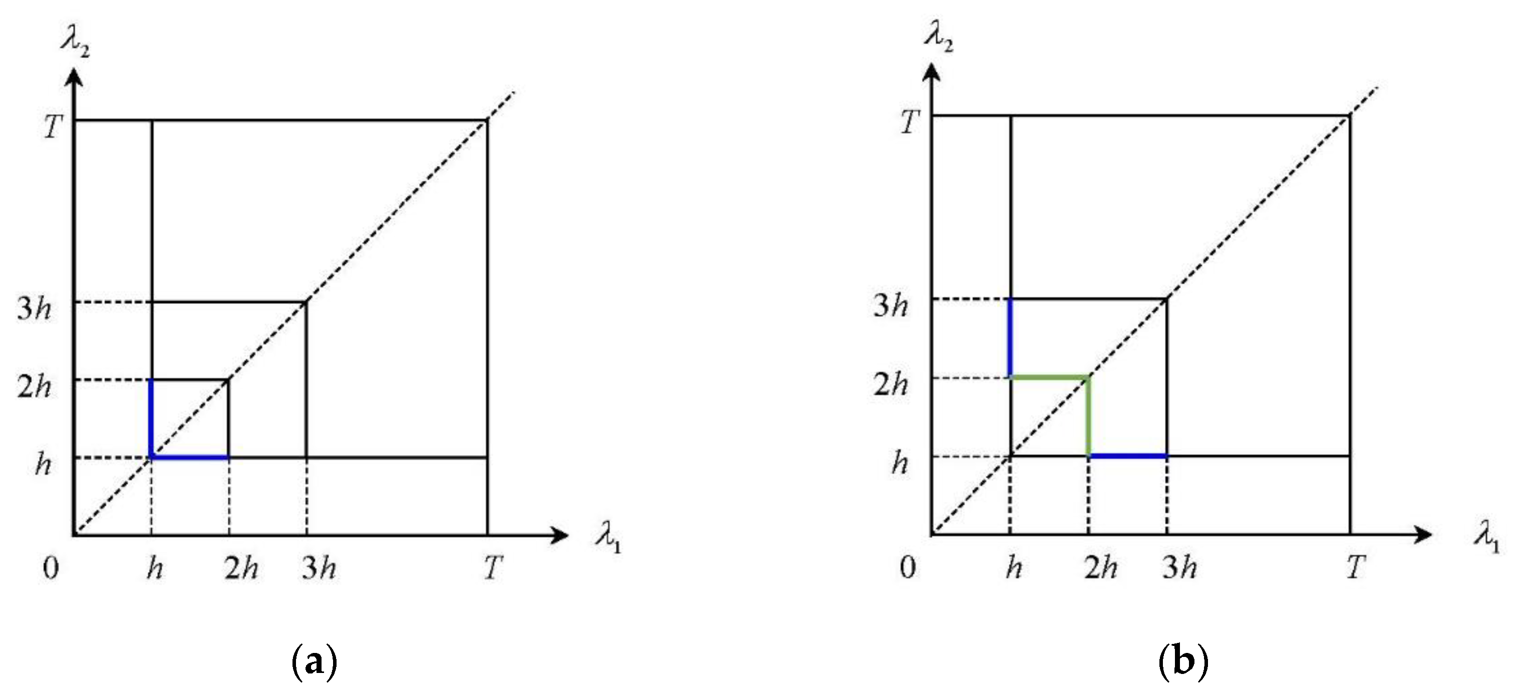
Lemma conditions (27)–(29) are standard conditions for the smoothness of the input data. Focusing on the geometric image of the domains ${\mathsf{\Delta }}_k$, we will illustrate the boundaries between the domains ${\mathsf{\Omega }}_k$ for the first values of $k=0, 1, 2$ (see Figure 5).

By analogy, it is easy to clarify the boundaries between the domains ${\mathsf{\Omega }}_k$ for other values of $k$. The proof is not particularly difficult, it can be carried out according to the scheme given in [49], and follows from geometric considerations. □

Theorem 1.

The Equations (27)–(29),

$$y_1\left(s_0,s_0\right)=y_2\left(s_0,s_0\right) \left(=y\left(s_0,s_0\right)\right), s_0\in \left[h,T\right],$$

(30)

$$y\left(h,h\right)=\underset{0}{\overset{h}{{\displaystyle \int }}}d{\lambda }_1\underset{0}{\overset{h}{{\displaystyle \int }}}{\phi }^{\left(0\right)}\left({\lambda }_1,{\lambda }_2\right)d{\lambda }_2,$$

(31)

$${{\left(y_1\right)}_{s_0{s}_1}^{\prime \prime }|}_{s_0=s_1=s}={{\left(y_2\right)}_{s_0{s}_1}^{\prime \prime }|}_{s_0=s_1=s^{\prime }} s\in \left[h,T\right]$$

(32)

are necessary and sufficient conditions for the existence of a solution for (19), (20), (24) in the class$C_{\Omega }$.

Proof of Theorem 1.

Necessity. Let $\overline{\phi }\left({\rm M}\right)\in C_{\mathsf{\Omega }}$ be a solution to (19), (20), (24). Then

$$y_1\left(s_0,s_1\right)=\underset{s_0-h}{\overset{s_0}{{\displaystyle \int }}}d{\lambda }_1\underset{s_1-h}{\overset{s_1}{{\displaystyle \int }}}\overline{\phi }\left({\lambda }_1,{\lambda }_2\right)d{\lambda }_2,$$

(33)

$$y_2\left(s_0,s_1\right)=\underset{s_1-h}{\overset{s_1}{{\displaystyle \int }}}d{\lambda }_1\underset{s_0-h}{\overset{s_0}{{\displaystyle \int }}}\overline{\phi }\left({\lambda }_1,{\lambda }_2\right)d{\lambda }_2.$$

(34)

From (29) and (33), it follows (30):

$$y_1\left(s_0,s_0\right)=y_2\left(s_0,s_0\right)=\underset{s_0-h}{\overset{s_0}{{\displaystyle \int }}}d{\lambda }_1\underset{s_0-h}{\overset{s_0}{{\displaystyle \int }}}\overline{\phi }\left({\lambda }_1,{\lambda }_2\right)d{\lambda }_2,$$

whence for $N\left(s_0,0\right)\in {∆}_1$, we have

$$\begin{gathered} \underset{h}{\overset{s_0}{{\displaystyle \int }}}d{\lambda }_1\underset{h}{\overset{s_0}{{\displaystyle \int }}}\overline{\phi }\left({\lambda }_1,{\lambda }_2\right)d{\lambda }_2=y\left(s_0,s_0\right)-\underset{s_0-h}{\overset{h}{{\displaystyle \int }}}d{\lambda }_1\underset{s_0-h}{\overset{h}{{\displaystyle \int }}}{\phi }^{\left(0\right)}\left({\lambda }_1,{\lambda }_2\right)d{\lambda }_2- \\ -\underset{s_0-h}{\overset{h}{{\displaystyle \int }}}d{\lambda }_1\underset{h}{\overset{s_0}{{\displaystyle \int }}}{\phi }^{\left(0\right)}\left({\lambda }_1,{\lambda }_2\right)d{\lambda }_2-\underset{h}{\overset{s_0}{{\displaystyle \int }}}d{\lambda }_1\underset{s_0-h}{\overset{h}{{\displaystyle \int }}}{\phi }^{\left(0\right)}\left({\lambda }_1,{\lambda }_2\right)d{\lambda }_2\equiv {\widehat{y}}_1\left(s_0,s_0\right). \end{gathered}$$

It can be seen that at the initial point $t_0=h$

$${\widehat{y}}_1\left(h,h\right)\equiv y\left(h,h\right)-\underset{0}{\overset{h}{{\displaystyle \int }}}d{\lambda }_1\underset{0}{\overset{h}{{\displaystyle \int }}}{\phi }^{\left(0\right)}\left({\lambda }_1,{\lambda }_2\right)d{\lambda }_2=0,$$

whence (31) follows immediately. Thus, the solution for (33) and (34) can be obtained by differentiating concerning $s_0,s_1$. Indeed,

$$\begin{array}{c}\overline{\phi }\left({\rm M}\right)={{\left(y_1\right)}_{s_0{s}_1}^{″}|}_{N\left(s_0,s_0-s_1\right)}+{\phi }^{\left(0\right)}\left(s_0-h,s_1\right)+{\phi }^{\left(0\right)}\left(s_0,s_1-h\right)-{\phi }^{\left(0\right)}\left(s_0-h,s_1-h\right), \\ {\rm M}\in {\mathsf{\Omega }}_1^{\left(1\right)}\left(N\left(s_0,s_0-s_1\right)\right), \end{array}$$

$$\begin{array}{c}\overline{\phi }\left(\overline{{\rm M}}\right)={{\left(y_2\right)}_{s_0{s}_1}^{″}|}_{N\left(s_0,s_0-s_1\right)}+{\phi }^{\left(0\right)}\left(s_1-h,s_0\right)+{\phi }^{\left(0\right)}\left(s_1,s_0-h\right)-{\phi }^{\left(0\right)}\left(s_1-h,s_0-h\right), \\ \overline{{\rm M}}\in {\mathsf{\Omega }}_1^{\left(2\right)}\left(N\left(s_0,s_0-s_1\right)\right). \end{array}$$

The continuity of $\overline{\phi }$ on ${\mathsf{\Omega }}_1={\mathsf{\Omega }}_1^{\left(1\right)}{\displaystyle \cup }{\mathsf{\Omega }}_1^{\left(2\right)}$ gives (27) and (32), and the continuity of ${\phi }^{\left(0\right)}$ on ${\mathsf{\Omega }}_0$ additionally implies (28) and (29). We denote $\overline{\phi }$ for $N\left(s_0,s_0-s_1\right)\in {∆}_1$ by ${\phi }^{\left(1\right)}$. Now, let $N\left(s_0,s_0-s_1\right)\in {∆}_2$. For $s_1=s_0$ we have:

$$\underset{2h}{\overset{s_0}{{\displaystyle \int }}}d{\lambda }_1\underset{2h}{\overset{s_0}{{\displaystyle \int }}}\overline{\phi }\left({\lambda }_1,{\lambda }_2\right)d{\lambda }_2=y\left(s_0,s_0\right)-\underset{s_0-h}{\overset{2h}{{\displaystyle \int }}}d{\lambda }_1\underset{s_0-h}{\overset{2h}{{\displaystyle \int }}}{\phi }^{\left(1\right)}\left({\lambda }_1,{\lambda }_2\right)d{\lambda }_2-$$

$$-\underset{s_0-h}{\overset{2h}{{\displaystyle \int }}}d{\lambda }_1\underset{2h}{\overset{s_0}{{\displaystyle \int }}}{\phi }^{\left(1\right)}\left({\lambda }_1,{\lambda }_2\right)d{\lambda }_2-\underset{2h}{\overset{s_0}{{\displaystyle \int }}}d{\lambda }_1\underset{s_0-h}{\overset{2h}{{\displaystyle \int }}}{\phi }^{\left(1\right)}\left({\lambda }_1,{\lambda }_2\right)d{\lambda }_2\equiv {\widehat{y}}_2\left(s_0,s_0\right).$$

Since

$${\widehat{y}}_2\left(2h,2h\right)\equiv y\left(2h,2h\right)-\underset{h}{\overset{2h}{{\displaystyle \int }}}d{\lambda }_1\underset{h}{\overset{2h}{{\displaystyle \int }}}{\phi }^{\left(1\right)}\left({\lambda }_1,{\lambda }_2\right)d{\lambda }_2=0,$$

then the solution for (33) and (34) can be obtained by differentiation concerning $s_0,s_1$, namely:

$$\begin{array}{c}\overline{\phi }\left({\rm M}\right)={{\left(y_1\right)}_{s_0{s}_1}^{\prime \prime }|}_{N\left(s_0,s_0-s_1\right)}+{\phi }^{\left(1\right)}\left(s_0-h,s_1\right)+{\phi }^{\left(1\right)}\left(s_0,s_1-h\right)-{\phi }^{\left(1\right)}\left(s_0-h,s_1-h\right), \\ {\rm M}\in {\mathsf{\Omega }}_2^{\left(1\right)}\left(N\left(s_0,s_0-s_1\right)\right), \end{array}$$

$$\begin{array}{c}\overline{\phi }\left(\overline{{\rm M}}\right)={{\left(y_2\right)}_{s_0{s}_1}^{\prime \prime }|}_{N\left(s_0,s_0-s_1\right)}+{\phi }^{\left(1\right)}\left(s_1-h,s_0\right)+{\phi }^{\left(1\right)}\left(s_1,s_0-h\right)-{\phi }^{\left(1\right)}\left(s_1-h,s_0-h\right), \\ \overline{{\rm M}}\in {\mathsf{\Omega }}_2^{\left(2\right)}\left(N\left(s_0,s_0-s_1\right)\right). \end{array}$$

The solution $\overline{\phi }$ for $N\left(s_0,s_0-s_1\right)\in {∆}_2$ is denoted by ${\phi }^{\left(2\right)}$. The continuity of $\overline{\phi }$ on ${\mathsf{\Omega }}_1{\displaystyle \cup }{\mathsf{\Omega }}_2$ implies conditions (27)–(29), (32). Repeating this process $N$ times, we obtain (27)–(29), (32) on the entire domain $\mathsf{\Omega }$, since $\mathsf{\Omega }={{\displaystyle \cup }}_{k=1}^{N+1}{\mathsf{\Omega }}_k$.

Sufficiency. Let conditions (27)–(32) be satisfied. Let us show that

$$\phi \left(s_0,s_1\right)={{\left(y_1\right)}_{s_0{s}_1}^{″}|}_{N\left(s_0,s_0-s_1\right)}+\phi \left(s_0,s_1-h\right)+\phi \left(s_0-h,s_1\right)-\phi \left(s_0-h,s_1-h\right)$$

and

$$\phi \left(s_1,s_0\right)={{\left(y_2\right)}_{s_0{s}_1}^{″}|}_{N\left(s_0,s_0-s_1\right)}+\phi \left(s_1-h,s_0\right)+\phi \left(s_1,s_0-h\right)-\phi \left(s_1-h,s_0-h\right)$$

define a continuous on $\mathsf{\Omega }$ solution $\overline{\phi }$ of the pair Equation (24) with prehistory (19) and (20). Indeed, the continuity of $\overline{\phi }$ on $\mathsf{\Omega }$ follows from (27)–(29), (32) [49]. Considering that $s_0\in \left[h,T\right]$, $s_1\ge h$, then we should consider the situations when $s_0\ne s_1$ and $s=s_0=s_1$ separately, since in the second case $V_{1,2}\phi =V_{2,1}\phi$ and so

$$\begin{array}{c}\begin{array}{c}\underset{s-h}{\overset{s}{{\displaystyle \int }}}d{\lambda }_1\underset{s-h}{\overset{s}{{\displaystyle \int }}}\phi \left({\lambda }_1,{\lambda }_2\right)d{\lambda }_2\end{array}=\underset{s-h}{\overset{s}{{\displaystyle \int }}}d{\lambda }_1\underset{s-h}{\overset{s}{{\displaystyle \int }}}\phi \left({\lambda }_2,{\lambda }_1\right)d{\lambda }_2=\\ =\frac{1}{2}\underset{s-h}{\overset{s}{{\displaystyle \int }}}\underset{s-h}{\overset{s}{{\displaystyle \int }}}\left(\phi \left({\lambda }_1,{\lambda }_2\right)+\phi \left({\lambda }_2,{\lambda }_1\right)\right)d{\lambda }_{1}d{\lambda }_2.\end{array}$$

(35)

For $s_0\ne s_1$, i.e., $s_0>s_1$ we have:

$$\begin{gathered} \begin{array}{c}{V}_{1,2}\overline{\phi }=\underset{s_0-h}{\overset{s_0}{{\displaystyle \int }}}d{\lambda }_1\underset{s_1-h}{\overset{s_1}{{\displaystyle \int }}}\left({\left(y_1\right)}_{{\lambda }_1{\lambda }_2}^{\prime \prime }+\phi \left({\lambda }_1,{\lambda }_2-h\right)+\phi \left({\lambda }_1-h,{\lambda }_2\right)-\phi \left({\lambda }_1-h,{\lambda }_2-h\right)\right)d{\lambda }_2=\end{array} \\ =y_1\left(s_0,s_1\right)-y_1\left(s_1-h,s_1\right)-y_1\left(s_0,s_1-h\right)+y_1\left(s_0-h,s_1-h\right)+ \\ +\underset{s_0-h}{\overset{s_0}{{\displaystyle \int }}}d{\lambda }_1\underset{s_1-h}{\overset{s_1}{{\displaystyle \int }}}\phi \left({\lambda }_1,{\lambda }_2-h\right)d{\lambda }_2+\underset{s_0-h}{\overset{s_0}{{\displaystyle \int }}}d{\lambda }_1\underset{s_1-h}{\overset{s_1}{{\displaystyle \int }}}\phi \left({\lambda }_1-h,{\lambda }_2\right)d{\lambda }_2- \\ -\underset{s_0-h}{\overset{s_0}{{\displaystyle \int }}}d{\lambda }_1\underset{s_1-h}{\overset{s_1}{{\displaystyle \int }}}\phi \left({\lambda }_1-h,{\lambda }_2-h\right)d{\lambda }_2=y_1\left(s_0,s_1\right), \end{gathered}$$

since

$$y_1\left(s_0-h,s_1\right)=\underset{s_0-h}{\overset{s_0}{{\displaystyle \int }}}d{\lambda }_1\underset{s_1-h}{\overset{s_1}{{\displaystyle \int }}}\phi \left({\lambda }_1-h,{\lambda }_2\right)d{\lambda }_2,$$

(36)

$$y_1\left(s_0,s_1-h\right)=\underset{s_0-h}{\overset{s_0}{{\displaystyle \int }}}d{\lambda }_1\underset{s_1-h}{\overset{s_1}{{\displaystyle \int }}}\phi \left({\lambda }_1,{\lambda }_2-h\right)d{\lambda }_2,$$

(37)

$$y_1\left(s_0-h,s_1-h\right)=\underset{s_0-h}{\overset{s_0}{{\displaystyle \int }}}d{\lambda }_1\underset{s_1-h}{\overset{s_1}{{\displaystyle \int }}}\phi \left({\lambda }_1-h,{\lambda }_2-h\right)d{\lambda }_2.$$

(38)

Using equalities similar to (36)–(38) for $y_2\left(s_0-h,s_1\right)$, $y_2\left(s_0,s_1-h\right)$, $y_2\left(s_0-h,s_1-h\right)$, it is easy to obtain $V_{2,1}\overline{\phi }=y_2\left(s_0,s_1\right)$. Let us turn further to the case . Taking into account (35), we have:

$$\begin{array}{c}{V}_{1,2}\phi \left(s,s\right)=V_{2,1}\phi \left(s,s\right)=\frac{1}{2}\underset{s-h}{\overset{s}{{\displaystyle \int }}}\underset{s-h}{\overset{s}{{\displaystyle \int }}}\left[{\left(y_1\right)}_{{\lambda }_1{\lambda }_2}^{″}+{\left(y_2\right)}_{{\lambda }_1{\lambda }_2}^{″}\right]d{\lambda }_{1}d{\lambda }_2+\\ +\underset{s-h}{\overset{s}{{\displaystyle \int }}}\underset{s-h}{\overset{s}{{\displaystyle \int }}}\left[\phi \left({\lambda }_1,{\lambda }_2-h\right)+\phi \left({\lambda }_1-h,{\lambda }_2\right)-\phi \left({\lambda }_1-h,{\lambda }_2-h\right)\right]d{\lambda }_{1}d{\lambda }_2=\\ =\frac{1}{2}{y}_1\left(s,s\right)+\frac{1}{2}{y}_2\left(s,s\right)=y\left(s,s\right)\end{array}$$

(at the end of the chain, we used condition (30) and equalities like (36)–(38)), which was to be proven. □

Theorem 2.

Let the conditions of Theorem 1 be satisfied and, in addition, the equalities

$$y_j\left(0,0\right)=0, j=1,2,$$

(39)

$$y_1\left(s_0,s_1\right)=y_2\left(s_1,s_1-s_0\right),$$

(40)

$$y_2\left(s_0,s_1\right)=y_1\left(s_1,s_1-s_0\right),$$

(41)

$${{\left(y_1\right)}_{s_1}^{\prime }|}_{s_0=s_1=s}={{\left(y_2\right)}_{s_0}^{\prime }|}_{s_0=s_1=s^{\prime }}$$

(42)

$${{\left(y_1\right)}_{s_0}^{\prime }|}_{s_0=s_1=s}={{\left(y_2\right)}_{s_1}^{\prime }|}_{s_0=s_1=s^{\prime }} s\in \left[h,T\right],$$

(43)

hold. Then, the solution to Equations (24), (19), and (20) in the class $C_{\Omega }$ is unique.

Proof of Theorem 2.

To prove Theorem 2, it suffices to show that the homogeneous equation

$${\left({\psi }_j\right)}_{s_0{s}_1}^{″}=0, j=1,2,$$

(44)

for the functions $y_1$, $y_2$,satisfying, in addition to (27)–(32), also (39)–(43), has only a trivial solution. Let us verify that (44) has only a trivial solution. The general solution of (44) is ${\psi }_j\left(s_0,s_1\right)={\eta }_j\left(s_0\right)+{\xi }_j\left(s_1\right)$, $j=1,2$, where ${\eta }_j,{\xi }_j$ are arbitrary functions of the class $C^2$.

Differentiate ${\psi }_j\left(s_0,s_1\right)$ concerning $s_0$ and $s_1$:

$${\left({\psi }_1\right)}_{s_0}^{\prime }={\eta }_1^{\prime }\left(s_0\right),{\left({\psi }_1\right)}_{s_1}^{\prime }={\xi }_1^{\prime }\left(s_1\right),{\left({\psi }_2\right)}_{s_0}^{\prime }={\xi }_2^{\prime }\left(s_0\right),{\left({\psi }_2\right)}_{s_1}^{\prime }={\xi }_2^{\prime }\left(s_1\right).$$

Hence, taking into account (42) and (43), we have ${{\xi }_1^{\prime }\left(s_1\right)|}_{s_1=s}={{\eta }_2^{\prime }\left(s_0\right)|}_{s_0=s}$ and ${{{\eta }_1^{\prime }\left(s_0\right)|}_{s_0=s}={\xi }_2^{\prime }\left(s_1\right)|}_{s_1=s}$, so

$${\xi }_1\left(s\right)-{\eta }_2\left(s\right)=c_1, {\eta }_1\left(s\right)-{\xi }_2\left(s\right)=c_2,$$

(45)

where $c_1$, $c_2$ are some constants. According to (40) and (41),

$${\eta }_1\left(s_0\right)+{\xi }_1\left(s_1\right)={\eta }_2\left(s_1\right)+{\xi }_2\left(s_1-s_0\right),$$

$${\eta }_2\left(s_0\right)+{\xi }_2\left(s_1\right)={\eta }_1\left(s_1\right)+{\xi }_1\left(s_1-s_0\right),$$

whence for $s_0=s_1=s$, we have the equalities:

$$\begin{array}{c}{\eta }_1\left(s\right)+{\xi }_1\left(s\right)-{\eta }_2\left(s\right)={\xi }_2\left(0\right),\\ {\eta }_2\left(s\right)+{\xi }_2\left(s\right)-{\eta }_1\left(s\right)={\xi }_1\left(0\right),\end{array}$$

(46)

which in view of (45) give

$${\eta }_1\left(s\right)={\xi }_2\left(0\right)-c_1, {\eta }_2\left(s\right)={\xi }_1\left(0\right)+c_2.$$

Therefore, ${\eta }_j\left(s\right)={\eta }_j$ are constants for any $s, j=1,2$. Then it follows from (46) that ${\xi }_j\left(s\right)={\xi }_j$ are also constants for arbitrary $s$ and $j=1,2$. Finally, taking into account (39), we obtain that ${\eta }_j+{\xi }_j=0$ and ${\psi }_j\left(s_0,s_1\right)\equiv 0$, $j=1,2$. □

Remark 1.

It is important to note that conditions (39)−(43) are not onerous. Indeed, if Equations (19), (20), and (24) are solvable in the class $C_{\mathsf{\Omega }}$, then (39)–(43) are automatically satisfied. In other words, if a solution to (19), (20), (24) exists in the class $C_{\mathsf{\Omega }}$, then it is unique.

Integral Equation (12) arises in the problem of identifying Volterra kernels when constructing mathematical models in the form of the Volterra polynomial. The theory of the Volterra series is widely used to describe nonlinear dynamic systems of the “input-output” type [51]. Numerical algorithms for (12), implemented in [52] based on the product integration method, have shown their effectiveness in modeling the dynamics of heat exchanger element.

5. Conclusions

The paper discusses applying the integral model of developing systems to determine strategies for the development of a large (aggregated) electric power system using the example of the Unified Energy System of Russia. The elements of the system belong to several age groups. We described two types of models that take into account the dynamics of the aging of elements in different ways. In model 1, from the system origin until the moment $T_1$, all elements of the system belong to the same group and work with the same efficiency. Each time at $T_i$, the age group $\left(i+1\right)$ appears. In model 2, the elements of the system from the system origin are divided into age groups that function with different efficiencies.

Calculations for two models on real-life data are presented. The results show that the proposed integral model can be used for a qualitative assessment of the strategies of system development. The developed model is designed to analyze the long-term forecast of the commissioning of generating capacities of a large EPS with various strategies for dismantling the generating equipment.

The existence and uniqueness theorem for the solution of the two-dimensional Volterra integral equation of the first kind with variable limits of integration is formulated and proven. The developed technique for obtaining a solution can be extended to the case of $n$-dimensional integral equations. The grid analogue of the two- and three-dimensional integral equations of the considered class was studied in connection with the identification of integrals of Volterra kernels using the product integration method [53].

References

- Ljung, L. System Identification: Theory for the User; Prentice Hall, Inc.: Hoboken, NJ, USA, 1987. [Google Scholar]
- Korbicz, J.; Koscielny, J.M. (Eds.) Modeling, Diagnostics and Process Control: Implementation in the DiaSter System; Springer: Berlin/Heidelberg, Germany, 2010. [Google Scholar] [CrossRef]
- Kler, A.M.; Zharkov, P.V.; Epishkin, N.O. Parametric optimization of supercritical power plants using gradient methods. Energy 2019, 189, 116230. [Google Scholar] [CrossRef]
- Zohuri, B. Heat Exchanger Types and Classifications. In Compact Heat Exchangers; Springer: Cham, Switzerland, 2017; pp. 19–56. [Google Scholar] [CrossRef]
- Levin, A.A.; Chistyakov, V.F.; Tairov, E.A. On application of the structure of the nonlinear equations system, describing hydraulic circuits of power plants, in computations. Bull. SUSU MMCS 2016, 9, 53–62. [Google Scholar] [CrossRef]
- Mota, F.A.S.; Carvalho, E.P.; Ravagnani, M.A.S.S. Modeling and Design of Plate Heat Exchanger. In Heat Transfer Studies and Applications; Kazi, S.N., Ed.; IntechOpen: London, UK, 2015; Available online: https://www.intechopen.com/books/heat-transfer-studies-and-applications/modeling-and-design-of-plate-heat-exchanger (accessed on 29 March 2021). [CrossRef] [Green Version]
- Dvorak, V. Advanced Methods of Modelling and Design of Plate Heat Exchangers. DEStech Trans. Environ. Energy Earth Sci. 2017. [Google Scholar] [CrossRef] [Green Version]
- Silva, C.D.S.; Liporace, F.S.; Queiroz, E.M. Fouling models for real time heat exchanger fouling detection. In Proceedings of the Selected papers from ENPROMER 2005—4th Mercosur Congress on Process Systems Engineering and 2nd Mercosur Congress on Chemical Engineering, Rio de Janeiro, Brazil, 14–18 August 2005. [Google Scholar]
- Kler, A.M.; Maksimov, A.S.; Stepanova, E.L. High-speed mathematical models of cogeneration steam turbines: Optimization of operation at heat and power plants. Thermophys. Aeromech. 2006, 13, 141–148. [Google Scholar] [CrossRef]
- Asadi, M.; Shokouhandeh, H.; Rahmani, F.; Hamzehnia, S.M.; Harikandeh, M.N.; Lamouki, H.G.; Asghari, F. Optimal placement and sizing of capacitor banks in harmonic polluted distribution network. In Proceedings of the 2021 IEEE Texas Power and Energy Conference (TPEC), College Station, TX, USA, 2–5 February 2021. [Google Scholar] [CrossRef]
- Shokouhandeh, H.; Ghaharpour, M.; Lamouki, H.G.; Pashakolaei, Y.R.; Rahmani, F.; Imani, M.H. Optimal estimation of capacity and location of wind, solar and fuel cell sources in distribution systems considering load changes by lightning search algorithm. In Proceedings of the 2020 IEEE Texas Power and Energy Conference (TPEC), College Station, TX, USA, 6–7 February 2020. [Google Scholar]
- Eremia, M.; Shahidehpour, M. (Eds.) Handbook of Electrical Power System Dynamics. Modeling, Stability, and Control; IEEE, Inc.: New York, NY, USA, 2013. [Google Scholar] [CrossRef]
- Senachin, P.K.; Briutov, A.A.; Senachin, A.P. Modelling of Physical and Chemical Processes and Combustion in Power Plants. Vol. 2. Models of Combustion Processes in Piston Engines; Polzunov Altai State Technical University: Barnaul, Russia, 2019. [Google Scholar]
- Tumanovskii, A.G.; Rezinskikh, V.F. The strategy of prolonging the service life and the technical reequipment of thermal power stations. Therm. Eng. 2001, 48, 413–439. [Google Scholar]
- Veselov, F.V.; Novikova, T.V.; Khorshev, A.A. Technological renovation of thermal power plants as a long-term check factor of electricity price growth. Therm. Eng. 2015, 62, 843–852. [Google Scholar] [CrossRef]
- Schwarz, H.-G. Modernisation of existing and new construction of power plants in Germany: Results of an optimisation model. Energy Econ. 2005, 27, 113–137. [Google Scholar] [CrossRef]
- Leontief, V. Studies in the Structure of the American Economy: Theoretical and Empirical Explorations in Input-Output Analysis; Oxford University Press: Oxford, UK, 1953. [Google Scholar]
- Lagerev, A.V. A dynamic territorial and production model for the development of scenarios of a mutually aligned development of Russia’s energy industry as concerns its federal subjects. Izv. RAN. Energ. 2004, 4, 26–32. [Google Scholar]
- Voropai, N.I.; Trufanov, V.V. Mathematical modeling of electric power system development in modern conditions. Elektrichestvo 2000, 10, 6–13. [Google Scholar]
- Vilensky, P.L.; Livshits, V.I.; Smolyak, S.A. Evaluation of the Effectiveness of Investment Projects. Theory and Practice; Delo: Moscow, Russia, 2001. [Google Scholar]
- Ghiani, E.; Mocci, S.; Pilo, F. Distribution System Reliability Assessment Considering Equipment Ageing. In Proceedings of the CIRED Conference, Vienna, Austria, 21–24 May 2007; p. 0392. [Google Scholar]
- Bragatto, P.; Catone, M.; Corrado, I.; Corrado, D.S.; Pirone, A.; Vallerotonda, M. Managing Pressure Equipment Aging in Plants with Major Accident Hazard: A Methodology Satisfying the Requirements of the European Directive 2012/18/UE Seveso III. In Proceedings of the ASME 2018 Pressure Vessels and Piping Conference, Prague, Czech Republic, 15–20 July 2018; Volume 7. [Google Scholar] [CrossRef]
- Vilchis-Rodriguez, D.; Levi, V.; Gupta, R.; Barnes, M. Feasibility Analysis of the Probabilistic Modelling of LCC Based HVDC Equipment Ageing Using Public Data. In Proceedings of the 10th International Conference PEMD 2020, Nottingham, UK, 1–3 December 2020. [Google Scholar]
- Ansaldi, S.; Bragatto, P.; Agnello, P.; Milazzo, M.F. An Ontology for the Management of Equipment Ageing. In Proceedings of the Conference ESREL2020 PSAM15, Venice, Italy, 1–5 November 2020. [Google Scholar] [CrossRef]
- Glushkov, V.M. On one class of dynamic macroeconomic models. Upravlyayushchie Sistemy Mashiny 1977, 2, 3–6. [Google Scholar]
- Apartsyn, A.S. Nonclassical Linear Volterra Equations of the First Kind; De Gruyter Publ.: Berlin, Germany, 2003. [Google Scholar] [CrossRef]
- Glushkov, V.M.; Ivanov, V.V.; Yanenko, V.M. Modeling of Developing Systems; Nauka: Moscow, Russia, 1983. [Google Scholar]
- Yatsenko, Y.P. Integral Models of Systems with Controllable Memory; Naukova Dumka: Kiev, Ukraine, 1991. [Google Scholar]
- Hritonenko, N.; Yatsenko, Y. Applied Mathematical Modeling of Engineering Problems; Kluwer Academic Publishers: Dortrecht, The Netherlands, 2003. [Google Scholar]
- Apartsin, A.S.; Trishechkin, A.M. Application of V.M. Glushkov models for modeling long-term strategies for development of the Unified Energy System. In Abstracts of the All-Union Conference “Kurs-4”; VINITI: Riga, Latvia, 1986; pp. 17–19. [Google Scholar]
- Apartsyn, A.S.; Trishechkin, A.M. Modeling of power system development on the base of integral descriptions. In EPRI-SEI Joint Seminar of Methods for Solving the Problems on Energy Power Systems Development and Control; Electric Power Research Institute: Beijing, China, 1991; pp. 133–143. [Google Scholar]
- Ivanov, D.V.; Karaulova, I.V.; Markova, E.V.; Trufanov, V.V.; Khamisov, O.V. Control and Power Grid Development: Numerical Solutions. Autom. Remote Control 2004, 65, 472–482. [Google Scholar] [CrossRef]
- Apartsin, A.S.; Karaulova, I.V.; Markova, E.V.; Trufanov, V.V. Application of the Volterra integral equations to the modeling of retooling strategies for electric power industry. Elektrichestvo 2005, 10, 69–75. [Google Scholar]
- Karaulova, I.V.; Markova, E.V. Optimal Control Problem of Development of an Electric Power System. Autom. Remote Control 2008, 69, 637–644. [Google Scholar] [CrossRef]
- Markova, E.V.; Sidler, I.V.; Trufanov, V.V. On models of developing systems and their applications. Autom. Remote Control 2011, 72, 1371–1379. [Google Scholar] [CrossRef]
- Markova, E.V.; Sidler, I.V.; Trufanov, V.V. Integral models of developing electric power systems. Int. J. Energy Optim. Eng. 2013, 2, 44–58. [Google Scholar] [CrossRef]
- Botoroeva, M.N.; Bulatov, M.V. Applications and Methods for the Numerical Solution of a Class of Integro-Algebraic Equations with Variable Limits of Integration. Bull. Irkutsk State Univ. Ser. Math. 2017, 20, 3–16. [Google Scholar] [CrossRef]
- Messina, E.; Russo, E.; Vecchio, A. A stable numerical method for Volterra integral equations with discontinuous kernel. J. Math. Anal. Appl. 2008, 337, 1383–1393. [Google Scholar] [CrossRef] [Green Version]
- Sidorov, D.N. On parametric families of solutions of Volterra integral equations of the first kind with piecewise smooth kernel. Differ. Equ. 2013, 49, 210–216. [Google Scholar] [CrossRef]
- Apartsin, A.S.; Sidler, I.V. Using the nonclassical Volterra equations of the first kind to model the developing. Autom. Remote Control 2013, 74, 899–910. [Google Scholar] [CrossRef]
- Apartsyn, A.S. To study the stability of solutions of test nonclassical Volterra equations of the first kind. Sib. Electron. Math. Rep. 2015, 12, 15–20. [Google Scholar]
- Apartsyn, A.S. On some classes of linear Volterra integral equations. Abstr. Appl. Anal. 2014, 2014, 532409. [Google Scholar] [CrossRef]
- Apartsyn, A.S.; Markova, E.V.; Sidler, I.V.; Trufanov, V.V. Optimization problem of equipment age structure in the model of Russia’s unified energy system development. In Proceedings of the 2017 International Multi-Conference on Engineering, Computer and Information Sciences, Hong Kong, China, 15–17 March 2017; pp. 24–29. [Google Scholar] [CrossRef]
- Markova, E.V.; Sidler, I.V. Numerical solution of the age structure optimization problem for basic types of power plants. Yugosl. J. Oper. Res. 2019, 29, 81–92. [Google Scholar] [CrossRef]
- Markova, E.; Sidler, I.; Trufanov, V. Optimization problem for the integral model of developing systems. J. Oper. Res. Soc. China 2020. [Google Scholar] [CrossRef]
- Novak, A.V. The Results of the Work of the Ministry of Energy of Russia and the Main Results of the Functioning of the Fuel and Energy Complex in 2015, Presentation for the Report of Minister of Energy of the Russian Federation. Available online: https://minenergo.gov.ru/modal/view-pdf/4913/60888/nojs (accessed on 25 March 2021).
- Apartsyn, A.S.; Sidler, I.V. Numerical solution of the Volterra equations of the first kind in integral models of developing systems. In Proceedings of the VII Intl Symp. “Generalized Statements and Solutions of Control Problems (GSSCP–2014)”, Moscow, Russia, 26–30 September 2014; pp. 21–25. [Google Scholar]
- Sidorov, D. Integral Dynamical Models. Singularities, Signals and Control; World Scientific Serieson Nonlinear Science; Series A: Monographs and Treatises, 87; World Scientific Publishing Co. Pte. Ltd.: Hackensack, NJ, USA, 2015. [Google Scholar] [CrossRef] [Green Version]
- Solodusha, S.; Antipina, E. Inversion formulas and their finite-dimensional analogs for multidimensional Volterra equations of the first kind. J. Phys. Conf. Ser. 2021, 1715, 012046. [Google Scholar] [CrossRef]
- El’sgol’ts, L.E.; Norkin, S.B. Introduction to the Theory and Applications of Differential Equations with Deviating Arguments; Academic Press: New York, NY, USA, 1973. [Google Scholar]
- Cheng, C.M.; Peng, Z.K.; Zhang, W.M.; Meng, G. Volterra-series-based nonlinear system modeling and its engineering applications: A state-of-the-art review. Mech. Syst. Signal Process. 2017, 87, 340–364. [Google Scholar] [CrossRef]
- Solodusha, S.V. To Identification of Integral Models of Nonlinear Multi-Input Dynamic Systems Using the Product Integration Method. Lect. Notes in Control Inf. Sci. in press.
- Solodusha, S.V. Quadratic and cubic Volterra polynomials: Identification and application. Vestnik St. Petersburg Univ. Appl. Math. Comput. Sci. Control Process. 2018, 14, 131–144. [Google Scholar] [CrossRef]
Figure 1.
The dynamics of commissioning of capacities of the EPS of Russia in prehistory (1950–2015) and the forecasting period (2016–2050), obtained using model 1.
Figure 2.
The dynamics of commissioning of capacities of the EPS of Russia in prehistory (1950–2015) and the forecasting period (2016–2050) in the vector case.
Figure 3.
The dynamics of commissioning of capacities of the EPS of Russia in prehistory (1950–2015) and the forecasting period (2016–2050), obtained using model 2.
Figure 4.
Geometric illustration of the location of the domains .
Figure 5.
Geometric illustration of the location of the boundaries between the domains : (a) The boundary between the domains and is highlighted in blue; (b) The boundary between the domains and is highlighted in blue, the boundary between the domains and is highlighted in green.
Publisher’s Note: MDPI stays neutral with regard to jurisdictional claims in published maps and institutional affiliations. |
© 2021 by the authors. Licensee MDPI, Basel, Switzerland. This article is an open access article distributed under the terms and conditions of the Creative Commons Attribution (CC BY) license (https://creativecommons.org/licenses/by/4.0/).
Share and Cite
MDPI and ACS Style
Markova, E.; Sidler, I.; Solodusha, S. Integral Models Based on Volterra Equations with Prehistory and Their Applications in Energy. Mathematics 2021, 9, 1127. https://0-doi-org.brum.beds.ac.uk/10.3390/math9101127
AMA Style
Markova E, Sidler I, Solodusha S. Integral Models Based on Volterra Equations with Prehistory and Their Applications in Energy. Mathematics. 2021; 9(10):1127. https://0-doi-org.brum.beds.ac.uk/10.3390/math9101127
Chicago/Turabian StyleMarkova, Evgeniia, Inna Sidler, and Svetlana Solodusha. 2021. "Integral Models Based on Volterra Equations with Prehistory and Their Applications in Energy" Mathematics 9, no. 10: 1127. https://0-doi-org.brum.beds.ac.uk/10.3390/math9101127
Note that from the first issue of 2016, this journal uses article numbers instead of page numbers. See further details here.