
An Analysis of Usage of a Multi-Criteria Approach in an Athlete Evaluation: An Evidence of NHL Attackers


Department of Public Economics, Faculty of Economics, VŠB—Technical University of Ostrava, Sokolská Třída 33, 70200 Ostrava, Czech Republic
Mathematics 2021, 9(12), 1399; https://0-doi-org.brum.beds.ac.uk/10.3390/math9121399
Submission received: 20 May 2021
/
Revised: 11 June 2021
/
Accepted: 15 June 2021
/
Published: 16 June 2021
(This article belongs to the Special Issue Multi-Criteria Decision Making and Data Mining)
Abstract
:The presented research focuses on the commonly used Technique for Order of Preference by Similarity to Ideal Solution (TOPSIS), which is applied to an evaluation of a basic set of 581 national hockey league (NHL) players in the 2018/2019 season. This is used in combination with a number of objective methods for weighting indicators for identifying differences in their usage. A total of 11 indicators with their own testimonial values, including points, hits, blocked shots and more, are selected for this purpose. The selection of a method for weighting indicators has a major influence on the results obtained and the differences between them, and maintains the internal links within the ranked set of players. Of the evaluated methods, we prefer the Mean Weight method, and we recommend that the input indicators be considered equivalent when evaluating athletes.
1. Introduction
Sports are among the largest sources of entertainment and, therefore, revenue in America. The top five most popular team sports are American football (the National Football League—NFL), baseball (Major League Baseball—MLB), basketball (the National Basketball Association—NBA), ice hockey (the National Hockey League—NHL) and football (Major League Soccer—MLS). They have been researched and examined by a range of authors focusing on marketing [1], television ratings [2], estimates of spending by persons attending sporting events [3], referees [4], marginal revenue product [5], the “superstar” effect [6], the effects of weather on attendance [7] and many other factors [7].
This paper covers the NHL, the premier hockey league in the world, and specifically the 2018/2019 season, which featured 31 teams: 24 from the United States and 7 from Canada [8]. Each of the teams plays 82 regular-season games, with the top 16 teams then advancing to the playoffs. Thanks to this number of games and the number of teams involved, there is an ample dataset available with detailed information about every team and the individual players. These data include commonly referenced statistics such as goals and assists, shots, games played, plus–minus, game-winning goals, hits, blocked shots, power play time on ice and many others that quantify the skills of individuals in minute detail and that are freely accessible (nhl.com accessed on 5 December 2020; tsn.ca).
While such a large volume of data is aggregated for individual players and teams, the most popular statistics in the media remain goals and assists and, in the case of goal keepers, save percentage [9,10]. This fact is confirmed by the NHL’s awards, given to the best of the best. A total of 20 individual awards are handed out annually to players, coaches and general managers [11]. The most important, which are typically awarded to offensive players, include awards for the most outstanding player as judged by members of the Professional Hockey Writers’ Association (Hart Trophy) and the most outstanding player in the regular season as judged by the members of the NHL Players’ Association (Ted Lindsay Award), along with the Art Ross Trophy for the league scoring champion (goals and assists combined). The Maurice Richard Trophy is awarded to the regular-season goal-scoring champion, the Calder Memorial Trophy to the best rookie player under 26 and the Conn Smythe Trophy to the most valuable player during the playoffs [11]. These awards are typically given on the basis of total points and, therefore, do not, in our opinion, fully capture the overall complexity of the players themselves, which is often very important. This myopic focus on the most visible indicators may be to the detriment of a large group of players. These are largely referred to as team players, who are willing to do the less visible work to help their more productive teammates succeed and excel.
From our point of view, it is not sufficient to choose the best players based on the total number of points achieved. It is necessary to consider other important factors/criteria (like plus–minus, hits, blocked shots and others). Therefore, the purpose of this paper was to introduce Multi-Criteria Decision-Making (MCDM) methods and their possible usage into the area of sports (as a possible advantage in managerial decision-making). This new perspective on sports can be widely applied in the selection of players (drafts, trades) or player ratings (contracts). The objective of this research was to use the selected MCDM method and TOPSIS (Technique for Order of Preference by Similarity to Ideal Solution) to comprehensively evaluate the performance of NHL offensive players and map their performance using multiple attributes. This research is divided into multiple sections for this purpose. The NHL, which is a highly contemporaneous topic that represents a large source of information for various types of research, is the subject of the second section. The third section presents TOPSIS as the primary tool for comprehensive assessment of a selected group of NHL players. Attention is focused in this section on five selected methods for weighting input parameters, the selection and influence on the overall results of which are quantified in the fourth section. This section is preceded by the research methodology, which describes in detail the procedure for selecting the parameters, the research sample and the apparatus of mathematical–statistical methods used in this process. The fifth section, represents the results of the completed analysis devoted to the application of the individual methods for weighting the monitored attributes combined with the TOPSIS technique. The final sections, the discussion and conclusion, summarizes the results within the context of the restrictions of the completed research and potential opportunities for its continuation.
2. National Hockey League from Different Points of View
Currently, a large group of authors are devoted to studying hockey and the NHL from different points of view. Booth et al. [12], Farah et al. [13] and Madsen et al. [14] explored the application of a mathematical programming approach to the expansion of NHL draft optimization and to the factors contributing to elite hockey players’ decisions, exploring variations in the production of NHL draftees. Nandakumar and Jensen [15] analyzed the unique challenges of quantitatively summarizing the game of hockey and highlighted how deficiencies in existing methods of evaluation shaped major avenues of research and the creation of new metrics. Chiarlitti et al. [16] evaluated draft-eligible players based on body composition, speed, power and strength. Farah et al. [13] explored whether population density and proximity to Canadian Hockey League teams were associated with the number of draftees produced. Depken et al. [17] analyzed the determinants of career length in the league.
Much attention is also paid to the field of medicine (e.g., incidence of traumatic brain injuries during contact sports, including in the NHL; see [18]). Navarro et al. [19] examined the effects of concussions on individual players in the National Hockey League (NHL) by assessing career length, performance and salary. Other authors used positional comparisons to assess the impact of fatigue on movement patterns in hockey [20], the utility of using visible signs (VS) of concussion in predicting a subsequent diagnosis of concussion in players [21] and other aspects of the NHL, especially in terms of health impacts on players [22,23].
From our point of view, there is another interesting group of authors who are looking at the NHL from an economic perspective and analyzing its microeconomic and macroeconomic impacts. An example would be the study of Treber et al. [24], which considered that labor-related work stoppages in professional sports could have the potential to alienate fans; however, whether they generate sustained reductions in demand remains an open question (an evaluation of lockouts that took place during 1994–1995, 2004–2005 and 2012–2013). Ge and Lopez [25] found limited evidence of enhanced productivity among European players and no evidence of a benefit or drawback for North American players. Using the impact of an NHL lockout on a county with an NHL team relative to trends in the surrounding counties, Jasina and Rotthoff [26] found no general impact on employment; however, we did find a decrease in payroll in some sectors. Marketing aspects of sponsorship were evaluated by O’Reilly et al. [27] and Bragg et al. [28]. The research of O’Reilly et al. [29] explored the drivers of merchandise sales in professional sports and provided the direction on key antecedents. Brander and Egan [30] showed that NHL player salaries exhibit a strong seniority-based wage structure, as performance-adjusted salaries rise significantly with age for most of the relevant range, peaking at about age 32 and onward. NHL players commonly miss time due to injury, which creates a substantial burden in lost salary costs [31].
As can be seen from the above literature review, the NHL is a current topic that has been addressed by several studies in the fields of medicine, economics, marketing, psychology, etc. The game itself, as a source of information for multi-criteria evaluation, is discussed in the following section.
National Hockey League as a Big Data Source
The result and course of a game is influenced by several factors. Franjkovic and Matkovic [32] aimed to determine which variables affected the final outcome more in situational parameters. One of the conclusions of this study is that save percentage contributes the most to the final result. Good teams usually have a better defense setup to eliminate shots in front of the net and a slot position to help goaltenders to have an open shot from a distance. Cyrenne [33] examined the relationship between a team’s salary distribution and its winning percentage and found evidence of a superstar effect, in that teams with a higher maximum player salary have higher winning percentages. According to Schulte et al. [34], Markov Game Model validation showed that total team action and state value provide a strong predictor of team success, as measured by the team’s average goal ratio. An evaluation of the other aspects of the NHL was analyzed by Friesl et al. [35]. Bowman et al. [36] indicated that competitive balance in the National Hockey League increased rather substantially during this period, and that overtime rules and shootouts have had a much larger positive impact on the competitive balance in the NHL than overtime approaches have had on the competitive balance of any of the other sports examined. Hoffmann et al. [37] investigated the magnitude of the home advantage, as games proceeded from regulation, to overtime, to the shootout, while adjusting for team quality. The shootout may affect the psychological and behavioral states of home-team players, generally resulting in a decrease in the home team’s odds of winning in the shootout relative to overtime. Beaudoin et al. [38] showed that there are various situational effects associated with the next penalty call, related to the accumulated penalty calls, the goal differential, the stage of the match and the relative strengths of the two teams. They also investigated individual referee effects across the NHL. Camire [39] examined the benefits, pressures and challenges of leadership and captaincy in the NHL. Different aspects were analyzed by Rockerbie [40], who estimated the effect of fighting in hockey games on attendance in the NHL from the 1997–1998 season through to the 2009–2010 season. Lopez [41] found that in the current points system, several teams are playing a significantly higher proportion of overtime games against non-conference opponents than in-conference ones, and that overtime games are also significantly more likely to occur in the months leading up to post-season play.
Gu et al. [42] considered how to use all available data and describe an expert system for predicting NHL game outcome (with 77.5% accuracy). In each system, the essential component is the system element, which, in this case, is players (see [43,44]). Our research is focused on evaluating the performance of NHL players as well as their comprehensive evaluation using MCDM methods in this field.
3. Technique for Order of Preference by Similarity to Ideal Solution
TOPSIS is defined by Zavadskas et al. [45] as being the second most widely used MCDM method. Others, the use of which is noted, for instance, by Tramarico et al. [46], include the Analytical Hierarchy Process (AHP), Analytic Network Process (ANP), Multi-Attribute Utility Theory (MAUT), Preference Ranking Organization Method for Enrichment Evaluations (PROMETHEE) and Elimination and Choice Expressing Reality (ELECTRE). Its origin may be traced back to Hwang and Yoon [47] and Yoon [48], who developed this technique as an alternative to the ELECTRE method mentioned above (see Figure 1).
Streimikine et al. [49] described the result of this technique as the solution with the shortest distance to the positive ideal solution (PIS) calculated using the Euclidean distance. This opinion was elaborated by other groups of authors (e.g., [45]), according to whom this method offers a solution that is, under the given conditions, closest to the above-mentioned PIS, while at the same time being farthest from the negative ideal solution (NIS). In Figure 1, to which Vavrek [50] refers in describing this method, each yellow ball represents one of the alternatives, while the red ball represents the NIS alternative and the green ball the PIS alternative. The best-ranked alternative (ball) is farthest from the grey ball (NIS) and closest to the black ball. The TOPSIS technique is calculated as per Vavrek and Bečica [51] and Vavrek et al. [52], but this research is not concerned with its more in-depth characteristics or an analysis of its calculation. These are readily available in the works of other authors, including Pavic and Novoselac [53], Seyedmohammadi et al. [54] and many others.
In every MCDM method, the first and one of the most important steps is the weighting of individual input indicators, and the TOPSIS technique is no exception. Keršuliene et al. [55] differentiate approaches to weighting into four basic groups: subjective, expert, objective and integrated (which represents a combination of the preceding approaches). Subjective methods reflect the personality of the decision-makers and their individual preferences (indicator weight is defined based on a subjective opinion). Expert evaluation, meaning evaluation by a group made up of a small number of experts in a given field, is covered by Kendall [56], Fisher and Yates [57], and the Fuller Method or the Fuller Triangle is typically used in this case. The final group, the group of objective methods, weights individual indicators based on a predefined mathematical model unique to each method, without any influence from the decision-maker on the result (the weight is given by the nature of the input data).
The focus of this research is to provide results to the professional community, influenced by the decision-maker (an individual’s subjectivity) to the lowest possible extent. Therefore, a total of five objective methods were selected for the needs of this research for weighting of the input indicators with various calculation processes, which should help accomplish this aim. The objective methods that are used together with the TOPSIS technique, and that are covered in more detail further on in this text, include:
- Coefficient of variance—CV;
- Criteria Importance Through Inter-Criteria Correlation—CRITIC;
- Mean Weight—MW;
- Standard Deviation—SD;
- Statistical Variance Procedure—SVP.
3.1. Selected Methods for Weighting Indicators
As mentioned above, several methods were selected for weighting the input indicators for the needs of calculation, using the TOPSIS technique. This section presents the five methods selected (CV, CRITIC, MW, SD and SVP), which are classified as objective methods. We consider the identified methods to be the root cause of the varied results produced within the completed research.
There are numerous uses for the coefficient of variance in the academic environment. The most frequent include its use in the form of momentary characteristics [58,59], CV control charts [60,61] and as a weighting method [62]. This research was completed using the calculation employed by Singla et al. [63]. An interesting fact is that the first step is the same as that specified by Yalcin and Unlu [64] for calculation using another of the employed methods, the CRITIC method. The CRITIC method is one of the most commonly used ones. It has applications in the environmental [65], medical [66], industrial and services fields [67,68]. The approach used for the CRITIC method calculation is based on the research of Yalcin and Unlu [64], who focused on the evaluation of an initial public offering (IPO) and divided this approach into three steps (data normalization, correlation calculation and weighting). For its extension and application to an offshore wind turbine technology selection process, see Narayanamoorthy et al. [69]. The MW method is the simplest in terms of its approach, given that the weight assigned to each indicator is the same. This method can be used when “no method” for weighting the individual indicators is being used, i.e., in situations where the monitored indicators are mutually equivalent [70]. The SD method involves weighting based on the variability of the individual indicators, i.e., basic momentary characteristics, the use of which is quite common in the academic world [71]. The highest weight is assigned to the indicator within which the greatest differences are found between the evaluated variants, i.e., the indicator with the greatest standard deviation. Ouerghi et al. [72] provide uses for this method. The SVP method operates in a manner similar to the SD method and weights each indicator based on variance. Its applications are covered, for instance, by Nasser et al. [73] and Tayali and Timor [74]. The application of other methods can be found in the research of Geetha et al. [75], Narayanamoorthy et al. [76] and Ramya [77].
As can be seen, the principle behind the calculation of each of these methods is different, and they all follow different data aspects or characteristics.
4. Methodology
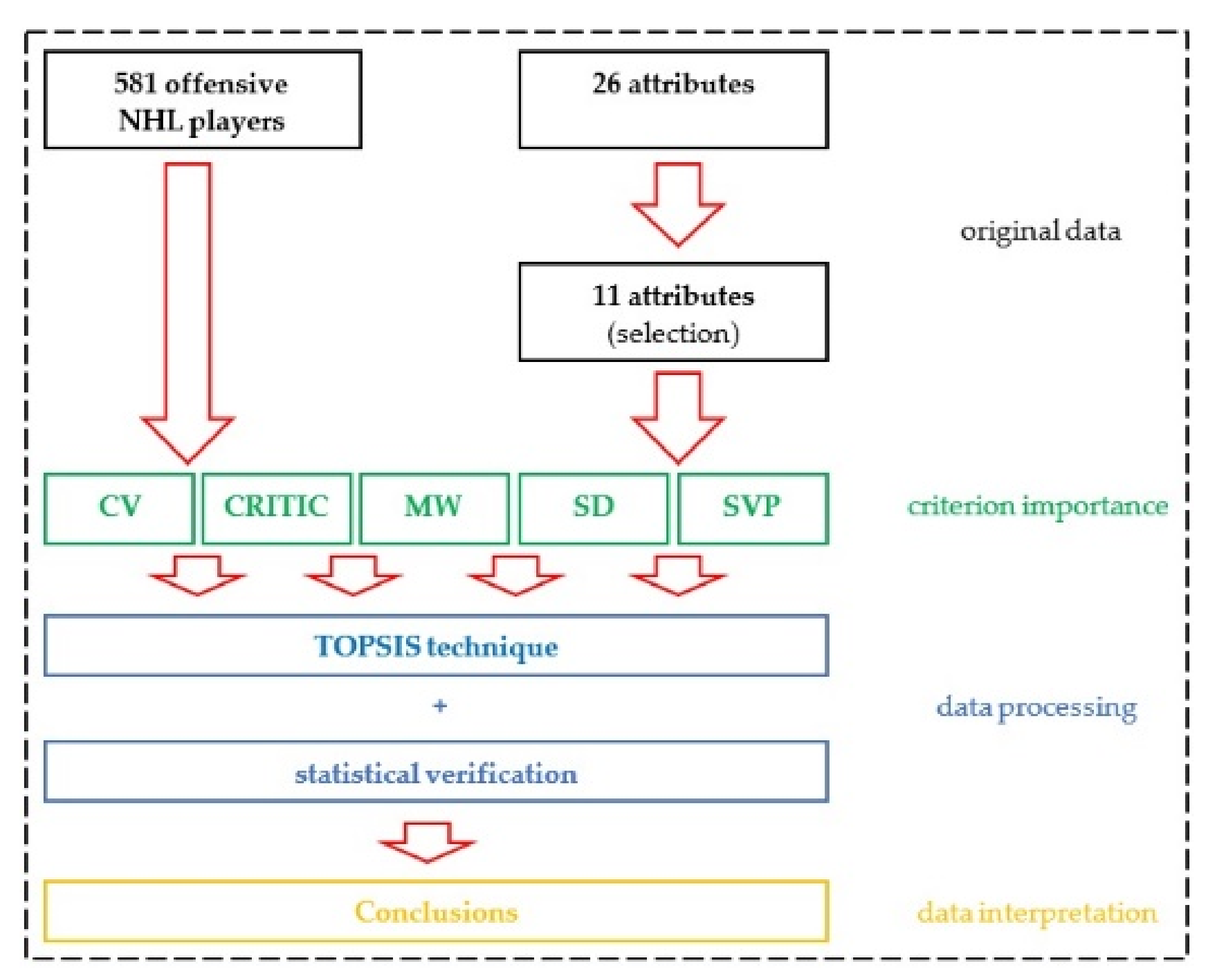
The objective of this research was to perform a comprehensive evaluation of NHL players’ performance regardless of their salary, marketability or any aspects other than those that are directly related to the game itself. The process is illustrated in the following figure (Figure 2).
A total of 11 attributes were selected (Section 4.1) to accomplish such an evaluation; we consider them to be the most important performance indicators that are monitored in practice. These indicators were monitored in a group of 518 offensive NHL players who were included in the statistics provided for individual players on the league’s official website (Section 4.2). The results from the application of the TOPSIS technique and the five methods for weighting the individual attributes are statistically verified and described in Section 4.3.
The objective was not to identify the best player in the NHL. The result of our analysis represents an assessment of the real application of multi-criteria evaluation on this group of NHL players and an identification of differences based on the use of various methods to determine the importance of the attributes applied.
4.1. Attribute Selection
The first phase involved work with the 26 individual data criteria published on the website www.nhl.com, with the goal of comprehensively depicting the performance of NHL offensive players in terms of offensive and defensive characteristics. All of the monitored attributes are absolute in nature and were recorded for the entire 2018/2019 regular season (see Table 1).
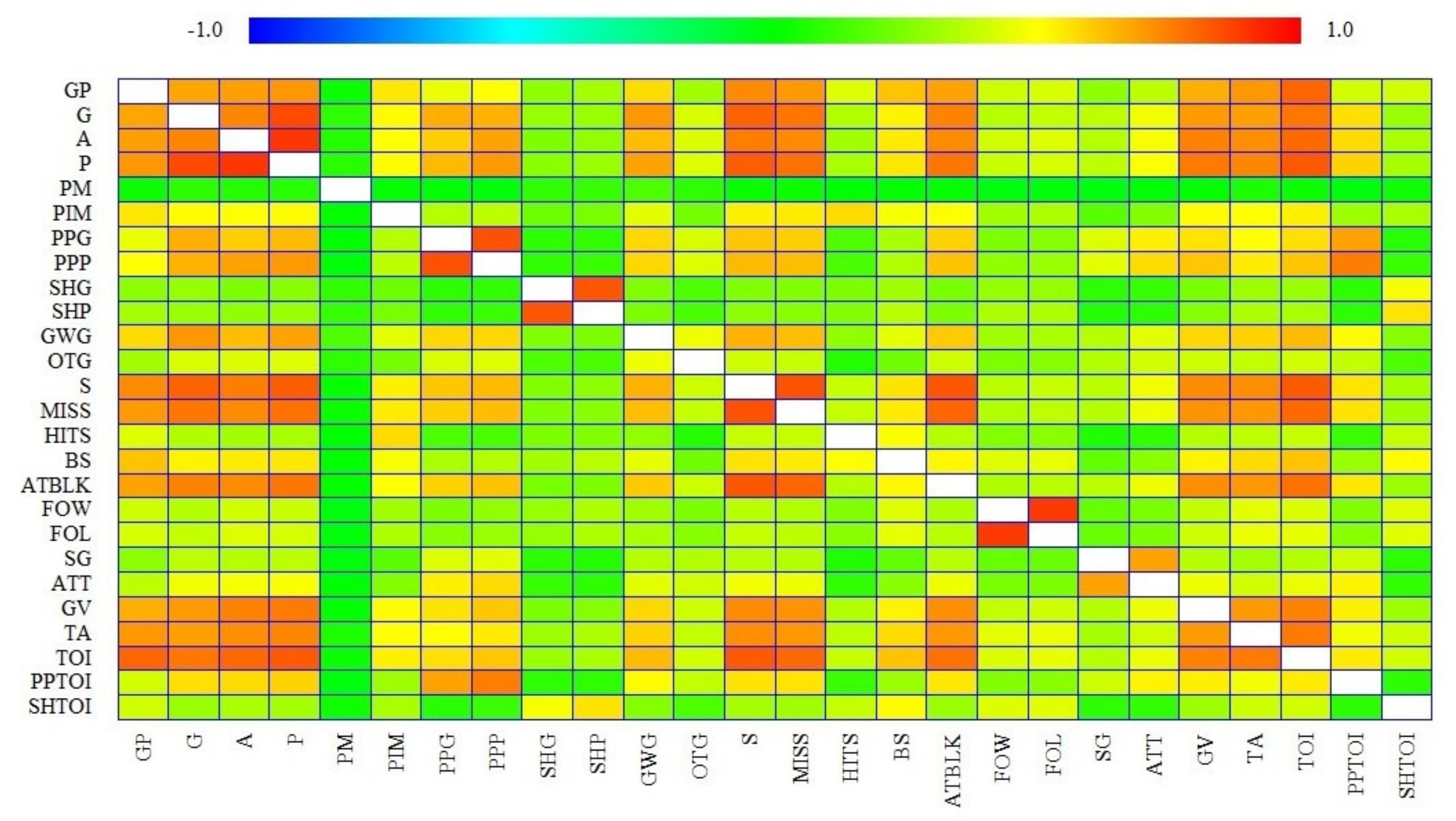
As noted above, the idea behind this research was to apply the TOPSIS technique to assess the performance of NHL players, while the aim was to apply attributes with a true testimonial value, meaning the lowest multi-collinearity of the input data. For this purpose, a linear order correlation (due to failure to meet the normal distribution condition) was calculated between the individual pairs of results, with the results captured in Figure 3.
Given the accepted level of a linear relationship (≤0.7), the majority of attributes whose structure and variability was duplicated with other monitored attributes were excluded from this group of attributes. The FOW or FOL attribute, which is dominant especially in the case of centers, given the logic of the game, was also excluded, as it could not be applied to the entire group of players (i.e., wings). The result of this selection was a group of 11 attributes that represent the input data for analysis using the TOPSIS technique (see Table 2).
The resulting structure of the monitored indicators sufficiently depicts, in our opinion, the accomplishment of both the offensive and defensive tasks of centers (C), as well as left (L) and right (R) wings.
4.2. Selected Methods for Weighting Indicators
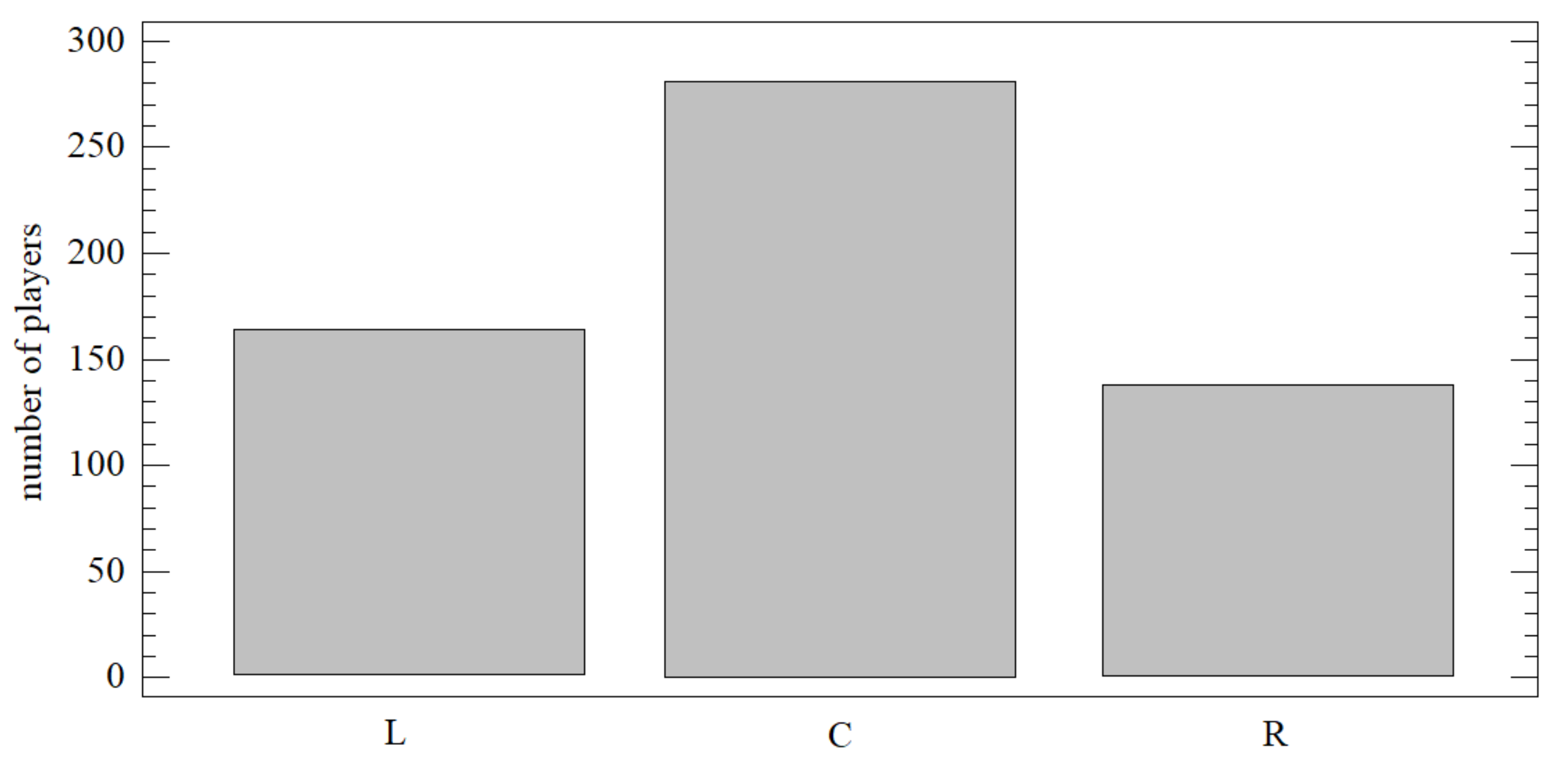
The set of players examined as specified in the evaluation methodology above includes all offensive players (C, L and R positions) who played in the 2018/2019 regular season and whose statistics are recorded on the NHL’s official website. There were 581 players in total, and their structure is specified below (see Figure 4).
To verify the testimonial value of the generated results, selected players who were nominated for certain awards for the 2018/2019 season were identified in the overall rankings (see Table 3). These are players who were nominated for at least 2 awards, specifically Nikita Kucherov, Connor McDavid and Patrick Kane, who were the top three players in terms of points at the end of the 2018/2019 regular season (assuming that none of them would be evaluated as the best by any of the combinations).
The performance of these players should be above average in the evaluated dataset, and they should be found near the top of the overall evaluation using the TOPSIS technique, regardless of the method applied for weighting the monitored attributes.
4.3. Methods of Processing and Statistical Verification of the Results Obtained
Analysis using the TOPSIS technique was completed a total of five times using the following methods for weighting the monitored attributes: CV, CRITIC, MW, SD and SVP (see Section 3). These results were then subjected to detailed statistical analysis, which included the following:
- The Kendall rank coefficient (rK)
- n—number of observations of a pair of variables;nc—number of concordant pairs;nd—number of discordant pairs.This was used for the initial monitoring of multi-collinearity between the individual attributes under consideration, as well as the linear relationship of these attributes with the overall results.
- The Kolmogorov–Smirnov test (K-S)
- —empirical distribution function of the first sample;
- —empirical distribution function of the second sample.
- The K-S test was used for verification of the conformity of the distribution functions of results obtained using the TOPSIS technique and individual methods for weighting the attributes.
- The Levene test (LE)
- k—number of values of the monitored categorical variable;
- N—number of observations;
- Ni—number of observations in the i-th group;
- Yij—measured value of the j-th unit of the i-th group;
- —average value of the i-th group;
- —median of the i-th group;
- —average of groups Zij;
- —average Zij for the i-th group.
- This test was used to verify the variance of these five results, i.e., verification of homoscedasticity.
- The Kruskal–Wallis test (Q) was used to verify the conformity of the mean of the results obtained:
- n—number of observations;
- ni—number of observations in the i-th group;
- —total number of orders in the i-th group.
- The Shapiro–Wilk test (S-W) to verify normal distribution of the distribution function of the results:
- n—number of observations;
- ni—empirical frequency;
- pi—theoretical probability that the values of a random variable lie in the i-th interval.
Multi-criteria evaluation using the TOPSIS technique and the weighting of the individual attributes was completed in MS Excel. Statistica 13.4 and Statgraphics XVIII software were used for statistical verification in the scope defined above and for graphic illustration purposes.
5. Results of Multi-Criteria Evaluation
The first section describes the different weights obtained through the application of the CV, CRITIC, MW, SD and SVP methods (Section 5.1). The results of the completed analysis are then divided into five separate sub-sections devoted to the application of the individual methods for weighting the monitored attributes combined with the TOPSIS technique (Section 5.2). The results are compared in the final section using the above-specified statistical apparatus (Section 5.3).
5.1. Comparison of the Importance of Weights by the Individual Methods
Weighting a monitored parameter is one of the steps in every multi-criteria method, including the TOPSIS technique, in which the weights are applied in the third step using a normalized criteria matrix. Their importance is covered, for example, by Vavrek [52], who assessed the impact of the selection of a suitable method for weighting monitored parameters on the overall results.
This research involved five objective methods for weighting the 11 monitored parameters, the result of which is depicted in Figure 5. This graphical illustration reveals significant and clear differences between the assigned weights, which are documented by the values of the coefficient of variance for every parameter at a level greater than 24% (vx ≥ 0.24), and a minimum standard deviation of sx ≥ 0.01963. The most significant differences in terms of the monitored parameters were observed in the case of short-handed time on ice (SHTOI) and HITS, for which the variance range was significantly different from that of the others (RHITS = 0.3239; RSHTOI = 0.3183). These results also contributed to rejecting the null hypothesis of the Levene test, i.e., confirming the heteroscedasticity of the weights of individual parameters (LE = 8.065; p < 0.01).
Significant differences also appear in terms of the individual methods and the distribution of 100% weight among the 11 parameters. Only the MW method shows an even distribution, which is of course given by its very name and especially the calculation itself. In such a case, all the parameters are equivalent and thus, insignificant, in terms of the TOPSIS technique (since there is multiplication by a constant, which does not change the structure of the data). The CV method came the closest to such an even distribution of weights, followed by the SVP method (note that the order of the specific parameters is not considered). In the former, the cumulative weight of the four most important parameters is 47.09% (36.3% in the case of MW), while the least important parameter has a weight of 2.32% (PM). In the SVP method, 79% of the importance is distributed between the SHTOI and HITS parameters, while the total weight of the last eight parameters is 6.89%. A higher number of overtime goals (in the OTG parameter) almost disappears from the results obtained using the method, as it is assigned a weight of only 0.005% (see Figure 6).
Given the above, it may be said that the selection of a method has a significant and clear impact on the results of the MCDM method, be it the TOPSIS technique or any other available method used in practice. The differences are so significant that they may substantially negate any attempt on the part of the decision-maker to select parameters with a clear testimonial value (without multi-collinearity), as was the case in the research provided (see Section 4.1). This conclusion was then verified in the evaluation of the overall results of the TOPSIS technique, combined with the CV, CRITIC, MW, SD and SVP methods for weighting.
5.2. Methods of Processing and Statistical Verification of the Results Obtained
This section briefly describes the results obtained using the TOPSIS technique combined with the five methods employed to define the importance of the input indicators, specifically the CV, CRITIC, MW, SD and SVP methods. Within each of them, attention is paid to identifying the best-rated players as well as differences compared to three award-winning players: Nikita Kucherov, Connor McDavid and Patrick Kane.
5.2.1. Results Obtained Based on the CV–TOPSIS Combination
Artemi Panarin (Columbus Blue Jackets) was identified as the best player based on the evaluation using the TOPSIS technique and the CV method for weighting the attributes (see Table 4). Overall, the rating of players is heterogeneous, using 60.06% of the potential variance range . A positive skew (γ1 = 1.189) indicates a higher number of below-average players, i.e., players with a result of ci < 0.1348 and rejection of the potential normal distribution of results (S-W = 0.890; p < 0.01).
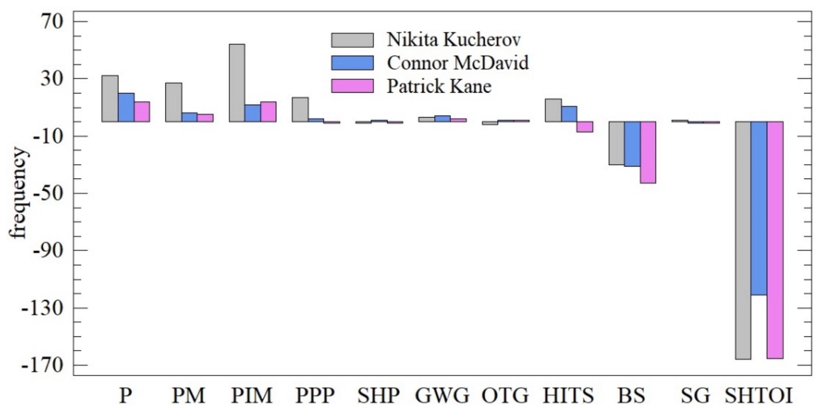
The best player as evaluated by the CV–TOPSIS combination in comparison to the three specified award-winning players (Kucherov, McDavid and Kane) exhibited better and more stable results in terms of individual parameters, meaning that he is among the best in most indicators. A significantly lower number of penalty minutes (PIM) ranks him higher than Kucherov, and his better plus/minus rating (PM) puts him ahead of McDavid and Kane. These differences ultimately influenced the overall ranking of the players (see Figure 7).
5.2.2. Results Obtained Based on the CRITIC–TOPSIS Combination
The second CRITIC–TOPSIS combination identified Aleksander Barkov (Florida Panthers) as the best player among the sample of 581 evaluated players, a ranking of whom is provided in Table 5. Differences in the evaluations of these players decreased (R = 0.5293), and there was a decrease in the skew of the results (γ1 = 0.314), which also indicates minimal differences in player rating and equalization of the overall score. Analysis of these results, given the results of the Shapiro–Wilk test, permits rejection of the hypothesis of their normal distribution (S-W = 0.954; p < 0.01).
Within the monitored attributes showing Aleksander Barkov as the highest-ranked player using the CRITIC–TOPSIS combination, there is a balance between a set of four indicators (SHP, GWG, OTG and SG), among which differences are minimal. Short-handed time on ice (SHTOI) is a clear differentiating factor compared to Kucherov, McDavid and Kane. These results underline the fact that the selected indicators are comprehensive and offer their own testimonial value (see Figure 8).
5.2.3. Results Obtained Based on the MW–TOPSIS Combination
Evaluation using the MW–TOPSIS combination provided the same result as the evaluation in the previous section and identified Aleksander Barkov (Florida Panthers) as the best player (see Table 6). Other parameters, specifically variance range and skew, show very similar values (γ1 = 0.266; R = 0.5151), which led to a rejection of the hypothesis of the normal distribution of the MW–TOPSIS results (S-W = 0.961; p < 0.01).
Identifying the same player as the de facto best means that the evaluation is similar to that in the previous Section 5.2.2, as the composition of the players remains unchanged.
5.2.4. Results Obtained Based on the SD–TOPSIS Combination
The most significant difference was the identification of Brandon Tanev (Winnipeg Jets) as the best or most effective player based on an evaluation of the 11 indicators (see Table 7). The differences between other players increased, which resulted in an increase in the overall variance range (R = 0.7176). A majority of the players delivered below-average results (ci < 0.2192), while the structure of these results did not have a normal distribution, as in the previous instances (S-W = 0.952; p < 0.01).
In the case of Brandon Tanev, the HITS and SHTOI indicators can be identified as the reason for his ranking. He is a fundamentally different kind of player (compared to Kucherov, McDavid and Kane) whose deficiencies on the offensive side are compensated by his defensive play, meaning his on-ice tasks are of a different nature (see Figure 9).
5.2.5. Results Obtained Based on the SVP–TOPSIS Combination
The trend identified while using the SD–TOPSIS combination concurred with the SVP–TOPSIS combination result. Brandon Tanev (Winnipeg Jets) was once again ranked first, his defensive efforts once again being the driving force (HITS, SHTOI). Significant differences were also identified between individual players (R = 0.800), while the evaluations of the three best players (see Table 8) can be described as outliers.
Identifying the same player as the de facto best means that the evaluation is similar to that in the previous Section 5.2.4, as the composition of the players remains unchanged. Once again, this result may be characterized as a rejection of the normal distribution of the results obtained (S-W = 0.925; p < 0.01).
5.3. Statistical Verification of the Results Obtained
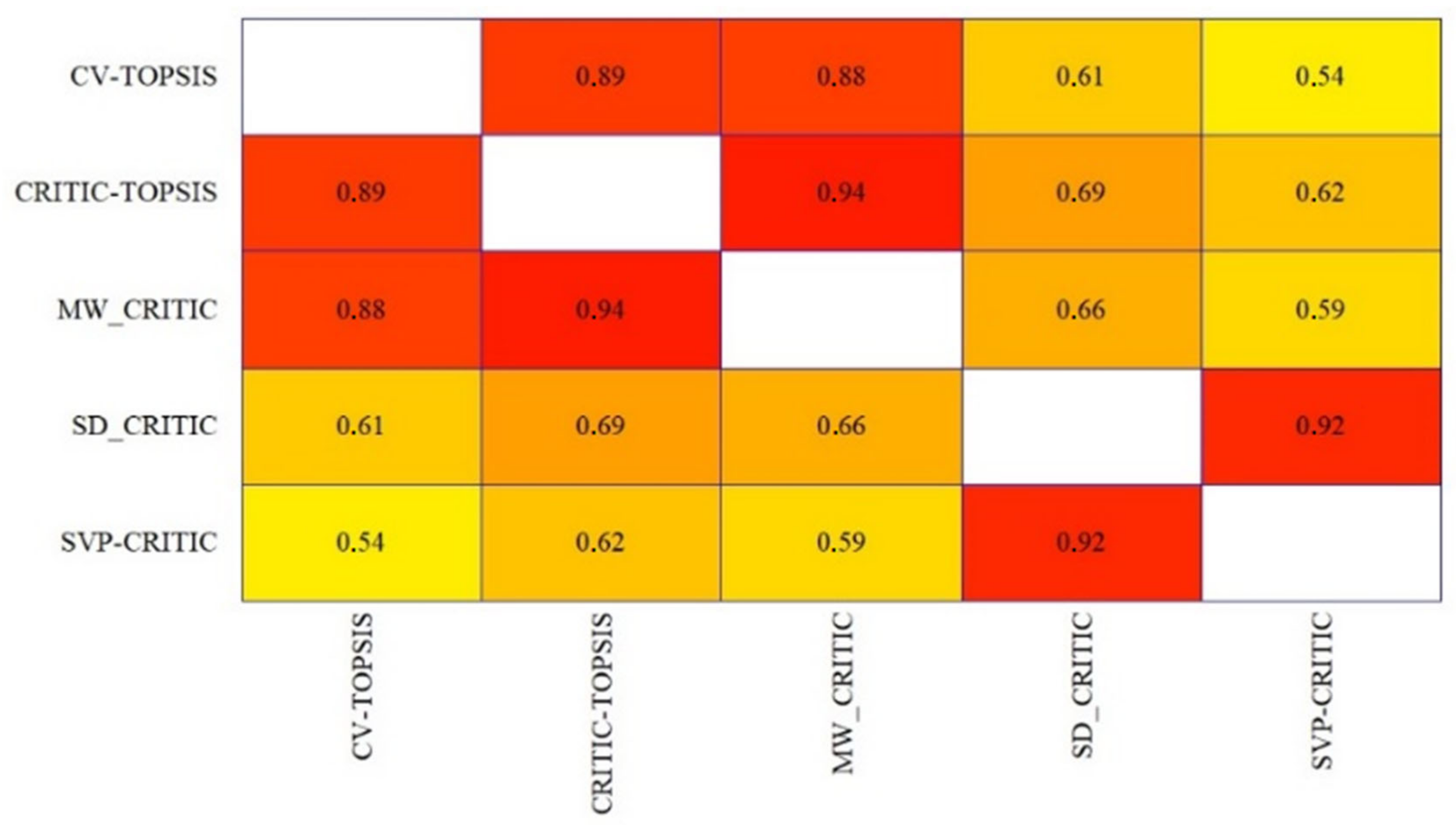
A comparison of the results obtained was completed from numerous perspectives with the goal of ascertaining the feasibility of using the TOPSIS technique to evaluate NHL players and any best combination for its actual implementation. In the first step, the testimonial value of the results obtained using the Kendall coefficient was compared to the following results (see Figure 10).
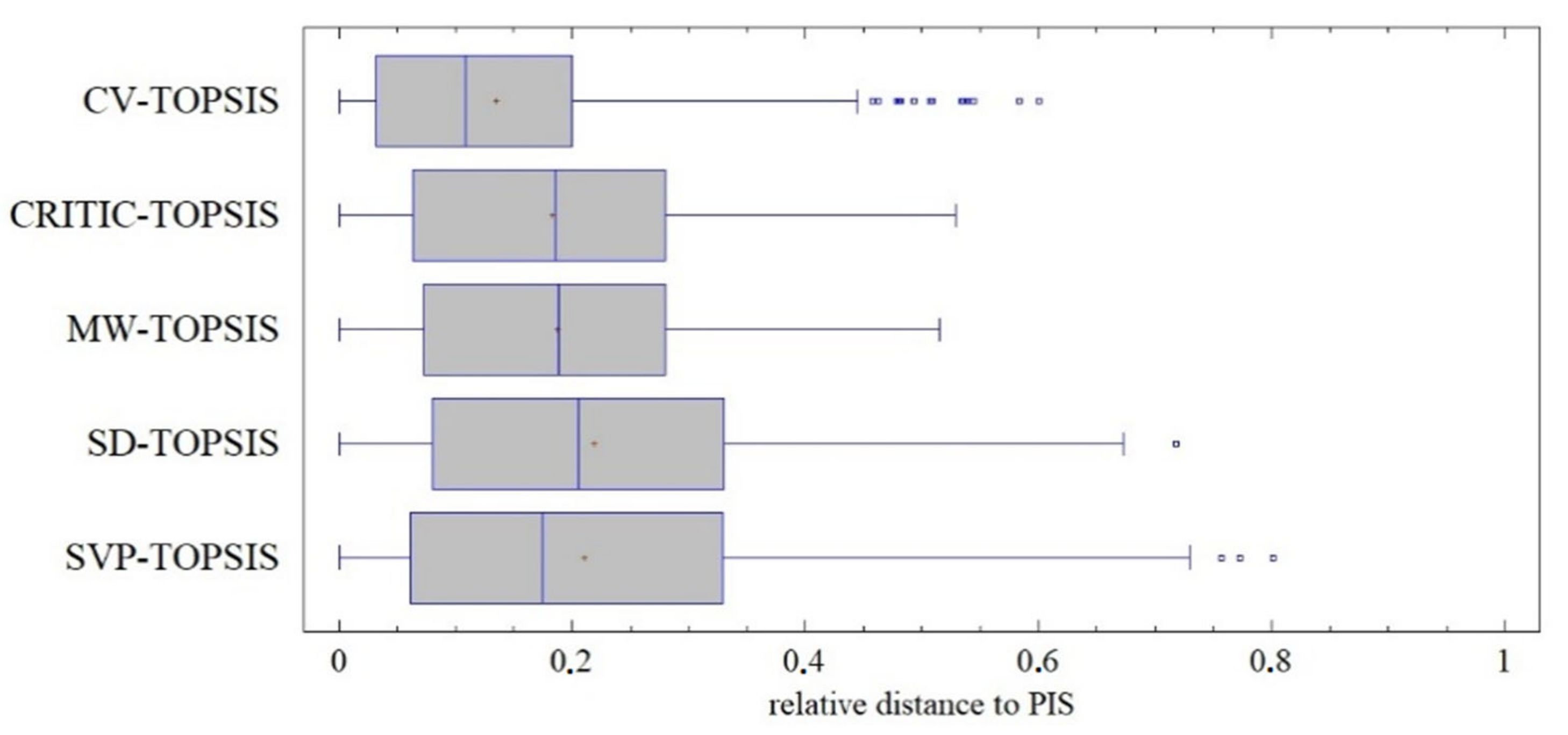
Figure 10 shows a high correlation between the pairs of results, namely the TOPSIS results obtained with CV–CRITIC, CV–MW, CRITIC–MW and SVP–SD. The alternation of these pairs may be considered, and therefore, the use of both would be superfluous from a methodological perspective. In the second step, the differences between selected momentary characteristics were compared and tested, specifically in terms of the mean value (Kruskal–Wallis test) and variance (Levene test), with the following results (see Figure 11).
Differences at the level of the variance range and the positions of the mean values (based on skew) are described in Section 5.2. In Figure 11, there are differences in variance (LE = 39.42; p < 0.01) and mean value (Q = 111.512; p < 0.01). Differences in the median are primarily observed for the CV–TOPSIS combination with other combinations, which were significant in all instances. In the next (third) step, the focus was on comparing the distribution functions of the results obtained using the Kolmogorov–Smirnov test, which confirmed the consistency of the distribution functions of the results obtained in two cases, namely CRITIC–MW (K-S = 0.645; p = 0.799) and SD–SVP (K-S = 1.32; p = 0.061). These results confirm the characteristics identified in Section 5.2 and the high correlation confirmed by the Kendall coefficient.
Figure 12 provides a closer examination of the overall results in terms of the individual positions (L, C and R). From a statistical perspective, there is no significant difference in the mean value (Q = 1.14; p = 0.565) or variance (LE = 0.139; p = 0.871) between the rankings for these positions, and their testimonial value is identical (rK = 1; p < 0.01).
Differences can be observed only between the individual methods—for instance, the best-rated left wings using the SD method for weighting the individual input indicators, etc. However, differences identified in this way are the same across all monitored positions, and therefore, it is not possible to assume either a positive or negative impact of the selected method on only certain subsets of the players analyzed.
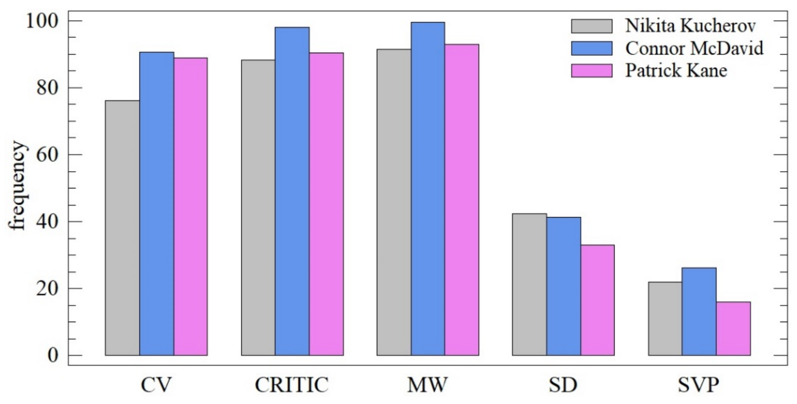
The ability to reflect a professional view of the quality of individual players was verified by the ranking of the three players (Kucherov, McDavid and Kane) in the evaluation of individual combinations, which is illustrated in Figure 13 and is, at first glance, markedly different.
Differences in the results produced by the individual methods appeared here as well. While the selected players were among the best in the TOPSIS combinations with CV, CRITIC and MW, they fell back to the average among the 581 NHL players in the SD and SVP combinations. The difference in results underlines the comparison of their evaluation compared to the ranking of the best player for the given combination, which once again emphasizes differences in the results obtained (see Figure 14).
6. Discussion
Any evaluation of the quality of a player in any sport is subject to various criteria and differences in perspectives among experts and the general public. How do we choose the best, and which criteria should be used to evaluate them? When considering only one league—in this case, the NHL— is the best player the one who scores the most goals (Maurice Richard Trophy) or the one who has the most points (Art Ross Trophy)? Or is the best player the one selected by the NHL Players’ Association (Ted Lindsay Award)? Today’s open world provides numerous potential answers to this question. Some try and identify the 10, 25, 50 or 100 best players [78,79,80,81], while others even select the 250 they consider the best [82]. There is also the ability to evaluate players based on their attributes in virtual reality or in video games (see [83]). Furthermore, there is an opinion that players should be evaluated not together, but instead by individual positions [84], etc. The only thing that these approaches have in common is the absence of any evaluation methodology. An evaluation method, a set of evaluation attributes and a method for calculating an overall evaluation, and therefore a final ranking, are completely lacking.
Of course, there have been attempts to take a quantitative approach to answering this question. One example is the research of Tarter et al. [85], who ranked players based on a set of 12 attributes, including goals per game, penalty minutes and physical parameters, such as height and weight. Macdonald [86] used four indicators, including goals and shots, to evaluate players. Von Allem et al. [87] used games played, goals and five other indicators. Other attempts can be found in the research of Chen et al. [88] and Qader et al. [89]. In composing a set of monitored indicators, our approach was based on this research, using 26 freely available indicators as the starting point. These were subjected to multi-collinearity testing to identify indicators with an independent testimonial value. The result was 11 evaluated attributes, which include points, penalty minutes, hits and others (see Table 2 for a complete list of the evaluated indicators), based on which the NHL players were evaluated within the provided research.
To evaluate the performance of players using this group of monitored indicators, the TOPSIS technique was selected, the application of which has been proven in numerous fields, including tourism [90], transportation [91], agriculture [54], risk assessment [92], the evaluation of cloud services providers [93] and the evaluation of local government entities [50]. One of the most important steps in every MCDM method, including TOPSIS, is weighting, or determining the importance of the evaluated indicators. To ensure that the analysis was not affected by our subjective outlook or subjectivity, we selected five objective methods for weighting the indicators: the CV, CRITIC, MW, SD and SVP methods. The selected methods are proven in practice and are unique and specific thanks to their individual approaches to calculation (see Section 3.1).
A difference in approach towards determining the importance of the selected indicators appeared in the first step of completing the analysis. Some methods, despite the individual testimonial value of the selected indicators, designated some of them as nearly unnecessary (such as OTG when the SVP method was used for weighting). Importance was most evenly distributed among the monitored indicators using the CV method (see Figure 6), which most closely approximated the MW method. This method considers the indicators to be equivalent (and there is no need to consider the importance of the indicators in this case).
Similar results were obtained using the MW and CRITIC methods and the SD and SVP methods. These pairs showed a high correlation of results (rK > 0.9) or a statistically significant match between their distribution functions. The generated results may be labeled as significantly different, especially in terms of two groups:
- The CV, CRITIC and MW methods, which primarily considered offensively skilled players to be the best when used within the TOPSIS technique, and which specifically identified Aleksander Barkov and Artemi Panarin as the best players;
- The SD and CVP methods, which primarily considered defensively skilled players to be the best when used within the TOPSIS technique, both of which identified Brandon Tanev as the best player.
7. Conclusions
A total of 581 NHL (offensive) players were evaluated in this research using a set of 11 indicators for the 2018/2019 regular season. These data were used for multi-criteria assessment using the TOPSIS technique and five objective methods to determine the importance of the input indicators (CV, CRITIC, MW, SD and SVP). These combinations produced significantly different results, which highlights the need for greater diligence when selecting a suitable method for weighting input indicators. This selection does not have an impact on the internal connections between the subjects of evaluation, which was shown in a comparison of the results by the players’ positions (see Figure 12). Based on the results obtained, we would favor one of the CV, CRITIC and MW methods for the purposes of evaluating athletes (as the subjects of evaluation). In this specific case, we have the greatest preference for the MW method and would consider the input indicators as equivalents for the purpose of multi-criteria evaluation. Therefore, we can recommend its usage in many problems requiring multiple criteria to be taken into account (not only in sports).
Further research can be carried out in three ways: (1) the results achieved can be processed via different methods (e.g., sensitivity analysis, factor analysis); (2) the group of objective weighting methods could be extended or compared with the results achieved using any subjective methods (e.g., the Fuller method); (3) the group of objective weighting methods could be applied on different MCDM methods (e.g., VIKOR, ELECTRE or PROMETHEE).
Funding
This research received no external funding.
Institutional Review Board Statement
Not applicable.
Informed Consent Statement
Not applicable.
Data Availability Statement
Publicly available datasets were analyzed in this study. This data can be found here: [https://www.nhl.com/], [https://www.tsn.ca/] (accessed on 5 December 2020).
Conflicts of Interest
The author declares no conflict of interest.
References
- Abeza, G.; Finch, D.; O’Reilly, N.; MacIntosh, E.; Nadeau, J. An Integrative Model of Sport Relationship Marketing: Transforming Insights Into Action. J. Sport Man. 2019, 33, 343–360. [Google Scholar] [CrossRef]
- Foster, G.; O’Reilly, N.; Shimizu, C.; Khosla, N.; Murray, R. Determinants of Regional Sport Network Television Ratings in MLB, NBA, and NHL. J. Sport Man. 2014, 28, 356–375. [Google Scholar] [CrossRef]
- Kelley, K.; Harrolle, M.G.; Casper, J.M. Estimating Consumer Spending on Tickets, Merchandise, and Food and Beverage: A Case Study of a NHL Team. J. Sport Man. 2014, 28, 253–265. [Google Scholar] [CrossRef]
- Duvinage, C.; Jost, P.C. The Role of Referees in Professional Sports Contests. J. Sports Econ. 2019, 20, 1014–1050. [Google Scholar] [CrossRef]
- Fort, R.; Lee, Y.H.; Oh, T. Quantile Insights on Market Structure and Worker Salaries: The Case of Major League Baseball. J. Sports Econ. 2019, 20, 1066–1087. [Google Scholar] [CrossRef]
- Humbhreys, B.R.; Johnson, C. The Effect of Superstars on Game Attendance: Evidence From the NBA. J. Sports Econ. 2019, 21, 152–175. [Google Scholar] [CrossRef]
- Ge, Q.; Humphreys, R.; Zhou, K. Are Fair Weather Fans Affected by Weather? Rainfall, Habit Formation, and Live Game Attendance. J. Sports Econ. 2019, 17–24. [Google Scholar] [CrossRef]
- Top 10 Most Popular Sports in America 2019 (TV Ratings). Available online: https://sportsshow.net/most-popular-sports-in-america/ (accessed on 5 December 2020).
- NHL Top Players. Available online: https://www.nhl.com/fans/nhl-top-players (accessed on 5 December 2020).
- TOP 10 Hokejistů pro Vstupní Draft NHL 2019. Bude Jedničkou Hughes Nebo Kakko? Available online: http://www.nhl.cz/top-10-hokejistu-pro-vstupni-draft-nhl-2019-bude-jednickou-hughes-nebo-kakko/5017893 (accessed on 11 January 2021).
- Trofeje NHL. Available online: http://nhlnews.cz/historie/trofeje-nhl/ (accessed on 3 December 2020).
- Booth, K.E.C.; Chan, T.C.Y.; Shalaby, Y. A mathematical optimization framework for expansion draft decision making and analysis. J. Quant. Anal. Sports 2019, 15, 27–40. [Google Scholar] [CrossRef]
- Farah, L.; Schorer, J.; Baker, J.; Wattie, N. Heterogeneity in Community Size Effects: Exploring Variations in the Production of National Hockey League Draftees Between Canadian Cities. Front. Psych. 2019, 9, 2746. [Google Scholar] [CrossRef]
- Madsen, R.; Smith, J.; Edwards, J.; Gentile, M.; Wayne, A. A fork in the road: Factors contributing to elite hockey players’ decisions to choose the NCAA route. Sport Soc. 2019, 23, 1235–1255. [Google Scholar] [CrossRef]
- Nandakumar, N.; Jensen, S.T. Historical Perspectives and Current Directions in Hockey Analytics. Ann. Rev. Stat. App. 2019, 6, 19–36. [Google Scholar] [CrossRef]
- Chiarlitti, N.; Delisie-Houde, P.; Reid, P.E.R.; Kennedy, C.; Andersen, R.E. Importance of Body Composition in the National Hockey League Combine Physiological Assessments. J. Strength Cond. Res. 2018, 32, 3135–3142. [Google Scholar] [CrossRef] [PubMed]
- Depken, C.A.; Ducking, J.; Groothuis, P.A. Career duration in the NHL: Pushing and pulling on Europeans? App. Econ. 2017, 49, 5923–5934. [Google Scholar] [CrossRef]
- Adams, R.; Kaye-Kauderer, H.; Haider, S.; Maniya, A.; Sobotka, S.; Choudhri, T. The effects of altitude on concussion incidence in the 2013-2017 National Hockey League seasons. Neurology 2018, 91, 16–17. [Google Scholar] [CrossRef] [Green Version]
- Navarro, S.M.; Pettit, R.W.; Haeberle, H.S.; Frangiamore, S.J.; Rahman, N.M.; Farrow, L.D.; Schickendantz, M.S.; Ramkumar, P.N. Short-Term Impact of Concussion in the NHL: An Analysis of Player Longevity, Performance, and Financial Loss. J. Neuro 2018, 35, 2391–2399. [Google Scholar] [CrossRef]
- Morencos, E.; Romero-Moraleda, B.; Castagna, C.; Casamichana, D. Positional Comparisons in the Impact of Fatigue on Movement Patterns in Hockey. Int. J. Sports Phys. Perf. 2018, 13, 1149–1157. [Google Scholar] [CrossRef] [PubMed]
- Echemendia, R.J.; Bruce, J.M.; Meeuwisse, W.; Hutchison, M.G.; Comper, P.; Aubry, M. Can visible signs predict concussion diagnosis in the National Hockey League? Brit. J. Sport Med. 2018, 52, 1149–1154. [Google Scholar] [CrossRef]
- Gebhard, C.E.; Gebhard, C.; Maafi, F.; Bertrand, M.J.; Stahli, B.E.; Wildi, K.; Galvan, Z.; Toma, A.; Zhang, Z.W.; Smith, D. Hockey Games and the Incidence of ST-Elevation Myocardial Infarction. Can. J. Cardio 2018, 34, 744–751. [Google Scholar] [CrossRef]
- Roy, J.; Forest, G. Greater circadian disadvantage during evening games for the National Basketball Association (NBA), National Hockey League (NHL) and National Football League (NFL) teams travelling westward. J. Sleep Res. 2018, 27, 86–89. [Google Scholar] [CrossRef] [Green Version]
- Treber, J.; Mulcahy, L.; Sharma, M.B. Empty Seats or Empty Threats? Examining the Effects of the 1994-1995 and 2004-2005 Lockouts on Attendance and Revenue in the National Hockey League. J. Sports Econ. 2016, 19, 395–677. [Google Scholar] [CrossRef]
- Ge, Q.; Lopez, M.J. Lockouts and Player Productivity: Evidence from the National Hockey League. J. Sports Econ. 2016, 17, 427–452. [Google Scholar] [CrossRef]
- Jasina, J.; Rotthoff, K. The Impact of the NHL Lockout on County Employment. Int. J. Sport Fin. 2016, 11, 114–123. [Google Scholar] [CrossRef] [Green Version]
- O’Reilly, N.; Stroebel, T.; Pfahl, M.; Kahler, J. An empirical exploration of sponsorship sales in North American professional sport Is it time to rethink our approach? Sport Bus. Man. Int. J. 2018, 8, 15–34. [Google Scholar] [CrossRef]
- Bragg, M.A.; Miller, A.N.; Roberto, C.A.; Sam, R.; Sarda, V.; Harris, J.L.; Brownell, K.D. Sports Sponsorships of Food and Nonalcoholic Beverages. Pediatrics 2018, 141, e20172822. [Google Scholar] [CrossRef] [PubMed] [Green Version]
- O’Reilly, N.; Foster, G.; Murray, R.; Shimizu, C. Merchandise sales rank in professional sport Purchase drivers and implications for National Hockey League clubs. Sport Bus. Man. Int. J. 2015, 5, 307–324. [Google Scholar] [CrossRef]
- Brander, J.A.; Egan, E.J. Seniority Wages in the National Hockey League. East. Econ. J. 2018, 44, 84–96. [Google Scholar] [CrossRef]
- Donaldson, L.; Li, B.; Cusinano, M.D. Economic burden of time lost due to injury in NHL hockey players. Inj. Prevent. 2014, 20, 347–349. [Google Scholar] [CrossRef] [PubMed]
- Franjkovic, A.; Matkovic, B. Effects of Game-Related Statistical Parameters on Final Outcome in National Hockey League (NHL). In Proceedings of the 8th International Scientific Conference on Kinesiology, Zagreb, Croatia, 10–14 May 2017; University of Zagreb: Zagreb, Croatia, 2017. [Google Scholar]
- Cyrenne, P. Salary Inequality, Team Success, League Policies, and the Superstar Effect. Cont. Econ. Pol. 2018, 36, 200–214. [Google Scholar] [CrossRef] [Green Version]
- Schulte, O.; Khademi, M.; Gholami, S.; Zhao, Z.Y.; Javan, M.; Desaulniers, P. A Markov Game model for valuing actions, locations, and team performance in ice hockey. Data Mining Knowl. Discov. 2017, 31, 1735–1757. [Google Scholar] [CrossRef]
- Friesl, M.; Lenten, L.J.A.; Libich, J.; Stehlik, P. In search of goals: Increasing ice hockey’s attractiveness by a sides swap. J. Operat. Res. Soc. 2017, 68, 1006–1018. [Google Scholar] [CrossRef]
- Bowman, R.A.; Lambrinos, J.; Ashman, T. Prospective measures of competitive balance application to money lines in the national hockey league. Appl. Econ. 2018, 50, 1925–4936. [Google Scholar] [CrossRef]
- Hoffmann, M.D.; Loughead, T.M.; Dixon, J.C.; Crozier, A.J. Examining the home advantage in the National Hockey League: Comparisons among regulation, overtime, and the shootout. Psych. Sport Exer. 2017, 28, 24–30. [Google Scholar] [CrossRef]
- Beaudoin, D.; Schulte, O.; Swartz, T.B. Biased penalty calls in the National Hockey League. Stat. Anal. Data Mining 2016, 9, 365–372. [Google Scholar] [CrossRef]
- Camire, M. Benefits, Pressures, and Challenges of Leadership and Captaincy in the National Hockey League. J. Clin. Sport Psych. 2016, 10, 118–136. [Google Scholar] [CrossRef]
- Rockerbie, D.W. Fighting as a profit maximizing strategy in the National Hockey League: More evidence. Appl. Econ. 2016, 48, 292–299. [Google Scholar] [CrossRef]
- Lopez, M.J. Inefficiencies in the National Hockey League Points System and the Teams That Take Advantage. J. Sports Econ. 2015, 16, 410–424. [Google Scholar] [CrossRef]
- Gu, W.; Saaty, T.L.; Whitaker, R. Expert System for Ice Hockey Game Prediction: Data Mining with Human Judgment. Int. J. Inf. Technol. Decis. Mak. 2016, 15, 763–789. [Google Scholar] [CrossRef]
- Burdekin, R.C.K.; Morton, M.G. Blood Money: Violence for Hire in the National Hockey League. Int. J. Sport Fin. 2015, 10, 328–356. [Google Scholar]
- Landry, J.; Edgar, D.; Harris, J.; Grant, K. National Hockey League guaranteed contracts A principal agent problem impacting on performance. Manag. Res. Rev. 2015, 38, 1306–1330. [Google Scholar] [CrossRef] [Green Version]
- Zavadskas, E.K.; Mardani, A.; Turskis, Z.; Jusoh, A.; Nor, K. Development of TOPSIS Method to Solve Complicated Decision-Making Problems: An Overview on Developments from 2000 to 2015. Int. J. Inf. Technol. Decis. Mak. 2016, 15, 1–38. [Google Scholar] [CrossRef]
- Tramarico, C.L.; Mizuno, D.; Antonio, V.; Salomon, P.; Augusto, F.; Marins, S. Analytic Hierarchy Process and Supply Chain Management: A Bibliometric Study. Proc. Comp. Sci. 2015, 55, 441–450. [Google Scholar] [CrossRef] [Green Version]
- Hwang, C.L.; Yoon, K. Multiple Attribute Decision Making, Methods and Applications; Springer: Berlin, Germany, 1981. [Google Scholar]
- Yoon, K. Systems Selection by Multiple Attribute Decision Making; Kansas State University: Kansas, MO, USA, 1980. [Google Scholar]
- Streimikiene, D.; Balezentis, T.; Krisciukaitiene, I.; Balezentis, A. Prioritizing sustainable electricity production technologies: MCDM approach. Renew. Sustain. Energy Rev. 2012, 16, 3302–3311. [Google Scholar] [CrossRef]
- Vavrek, R. Evaluation of the Impact of Selected Weighting Methods on the Results of the TOPSIS Technique. Int. J. Inf. Tech. Decis. Mak. 2019, 18, 1821–1843. [Google Scholar] [CrossRef]
- Vavrek, R.; Bečica, J. Capital City as a Factor of Multi-Criteria Decision Analysis—Application on Transport Companies in the Czech Republic. Mathematics 2020, 8, 1765. [Google Scholar] [CrossRef]
- Vavrek, R.; Papcunová, V.; Tej, J. Evaluation of Financial Management of Towns in relation to Political Cycles using CV-TOPSIS. Lex-loc. J. Loc. Self-Gov. 2020, 18, 231–252. [Google Scholar] [CrossRef]
- Pavic, Z.; Novoselac, M. Notes on TOPSIS Method. Int. J. Res. Eng. Sci. 2013, 1, 5–12. [Google Scholar]
- Seyedmohammadi, J.; Sarmadian, F.; Jafarzadeh, A.A.; Ghorbani, M.A.; Shahbazi, F. Application of SAW, TOPSIS and fuzzy TOPSIS models in cultivation priority planning for maize, rapeseed and soybean crops. Geoderma 2018, 310, 178–190. [Google Scholar] [CrossRef]
- Keršuliene, V.; Zavadskas, E.K.; Turskis, Z. Selection of rational dispute resolution method by applying new step-wise weight assessment ratio analysis (SWARA). J. Bus. Econ. Manag. 2010, 11, 243–258. [Google Scholar] [CrossRef]
- Kendall, M.G. Rank Correlation Methods; Griffin: London, UK, 1970. [Google Scholar]
- Fisher, R.A.; Yates, F. Statistical Tables for Biological, Agricultural and Medical Research; Oliver and Boyd: London, UK, 1963. [Google Scholar]
- Girling, A.J. Relative efficiency of unequal cluster sizes in stepped wedge and other trial designs under longitudinal or cross-sectional sampling. Stat. Med. 2018, 37, 4652–4664. [Google Scholar] [CrossRef] [PubMed] [Green Version]
- Thangjai, W.; Niwitpong, S.A. Confidence intervals for the weighted coefficients of variation of two-parameter exponential distributions. Cog. Math. 2017, 4, 1315880. [Google Scholar] [CrossRef]
- Tran, K.P.; Heuchenne, C.; Balakrishnan, N. On the performance of coefficient of variation charts in the presence of measurement errors. Qual. Reliab. Eng. Int. 2019, 35, 329–350. [Google Scholar] [CrossRef] [Green Version]
- Muhammad, A.N.B.; Yeong, W.C.; Chong, Z.L.; Lim, S.L. Monitoring the coefficient of variation using a variable sample size EWMA chart. Comp. Ind. Eng. 2018, 126, 378–398. [Google Scholar] [CrossRef]
- Bhowate, A.; Aware, M.; Sharma, S. Predictive Torque Control with Online Weighting Factor Computation Technique to Improve Performance of induction Motor Drive in Low Speed Region. IEEE Access 2019, 7, 42309–42321. [Google Scholar] [CrossRef]
- Singla, A.; Sing Ahuja, I.; Sing Sethi, A. Comparative Analysis of Technology Push Strategies Influencing Sustainable Development in Manufacturing Industries Using TOPSIS and VIKOR Technique. Int. J. Qual. Res. 2017, 12, 129–146. [Google Scholar]
- Yalcin, N.; Ünlü, U. A Multi-Criteria Performance Analysis of Initial Public Offering (IPO) Firms Using Critic and Vikor Methods. Tech. Econ. Dev. Econ. 2018, 24, 534–560. [Google Scholar] [CrossRef]
- Ighravwe, D.E.; Babatunde, D.E. Evaluation of landfill gas plant siting problem: A multi-criteria approach. Environ. Health Eng. Manag. J. 2019, 6, 1–10. [Google Scholar] [CrossRef]
- Jiang, S.H.; Zhang, Y.L.; Zhao, F.C.; Yu, Z.J.; Zhou, X.F.; Chu, H.Q. Impact of transmembrane pressure (TMP) on membrane fouling in microalgae harvesting with a uniform shearing vibration membrane system. Algal Res. 2018, 35, 613–623. [Google Scholar] [CrossRef]
- Kumari, M.; Kulkarni, M.S. Single-measure and multi-measure approach of predictive manufacturing control: A comparative study. Comp. Ind. Eng. 2019, 127, 182–195. [Google Scholar] [CrossRef]
- Tus, A.; Adali, E.A. The new combination with CRITIC and WASPAS methods for the time and attendance software selection problem. Opsearch 2019, 56, 528–538. [Google Scholar] [CrossRef]
- Narayanamoorthy, S.; Ramya, L.; Kang, D.; Baleanu, D.; Varghese, J.; Veerappan Annapoorani, K. A new extension of hesitant fuzzy set: An application to an offshore wind turbine technology selection process. IET Renew. Power Gener. 2021. [Google Scholar] [CrossRef]
- Xing, H.F.; Chen, Z.Y.; Zhang, X.X.; Yang, H.T.; Gou, M.F. Optimal Weighted Fusion Based on Recursive Least Squares for Dynamic North-Finding of MIMU on a Tilting Base. IEEE Access 2019, 7, 96215–96222. [Google Scholar] [CrossRef]
- Feng, Z.Y.; Cao, C.X.; Liu, Y.T.; Zhou, Y.L. A Multiobjective Optimization for Train Routing at the High-Speed Railway Station Based on Tabu Search Algorithm. Math. Prob. Eng. 2018, 2018, 8394397. [Google Scholar] [CrossRef] [Green Version]
- Ouerghi, H.; Mourali, O.; Zagrouba, E. Non-subsampled shearlet transform based MRI and PET brain image fusion using simplified pulse coupled neural network and weight local features in YIQ colour space. IET Image Process. 2018, 10, 1873–1880. [Google Scholar] [CrossRef]
- Nasser, A.A.; Alkhulaidi, A.A.; Mansoor, N.A.; Hankal, M.; Al-olofe, M. A Study on the Impact of Multiple Methods of the Data Normalization on the Result of SAW, WED and TOPSIS Ordering in Healthcare Multi-Attributtes Decision Making Systems based on EW, ENTROPY, CRITIC and SVP Weighting Approaches. Ind. J. Soc. Tech. 2019, 12, 99982. [Google Scholar] [CrossRef]
- Tayali, H.A.; Timor, M. Ranking with Statistical Variance Procedure based Analytic Hierarchy Process. Acta Info. 2017, 1, 31–38. [Google Scholar]
- Geetha, S.; Narayanamoorthy, S.; Manirathinam, T.; Kang, D. Fuzzy case-based reasoning approach for finding COVID-19 patients priority in hospitals at source shortage period. Exp. Syst. Appl. 2021, 178, 114997. [Google Scholar] [CrossRef]
- Narayanamoorthy, S.; Ramya, L.; Kalaiselvan, S.; Varghese Kureethara, J.; Kang, D. Use of DEMATEL and COPRAS method to select best alternative fuel for control of impact of greenhouse gas emissions. Soc. Econ. Plan. Sci. 2020, 100996. [Google Scholar] [CrossRef]
- Ramya, L.; Narayanamoorthy, S.; Kalaiselvan, S.; Varghese Kureethara, J.; Annapoorani, V.; Kang, D. A Congruent Approach to Normal Wiggly Interval-Valued Hesitant Pythagorean Fuzzy Set for Thermal Energy Storage Technique Selection Applications. Int. J. Fuzzy Syst. 2021, 1–19. [Google Scholar]
- Predicting the 10 Best NHL Players in the 2019–20 Season. Available online: https://bleacherreport.com/articles/2213535-predicting-the-10-best-nhl-players-in-the-2019-20-season#slide0 (accessed on 5 January 2021).
- Ranking the top 25 NHL forwards in 2019–20. Available online: https://www.sportingnews.com/us/nhl/news (accessed on 5 January 2021).
- NHL Rank: Predicting the 50 Best Players for the 2019–20 Season. Available online: https://www.espn.com/nhl/story/_/id/27653007/nhl-rank-predicting-50-best-players-2019-20-season (accessed on 6 January 2021).
- Top 100 NHL Players of 2018–19: The Full List. Available online: https://www.sportsnet.ca/hockey/nhl/top-100-nhl-players-2018-19-full-list/ (accessed on 6 January 2021).
- Fantasy Hockey top 200 Rankings for 2019–20. Available online: https://www.nhl.com/news/nhl-fantasy-hockey-top-250-rankings-players-2019-20/c-281505474 (accessed on 6 January 2021).
- NHL 19 Player Ratings Top 50. Available online: https://www.easports.com/nhl-19/ratings/nhl-19-player-ratings-top-50 (accessed on 6 January 2021).
- Official Websites. Available online: http://www.nhl.com/stats/ (accessed on 16 November 2020).
- Tarter, B.; Kirisci, L.; Tarter, R.; Jamnik, V.; Gledhill, N.; McGuire, E.J. Use of the Sports Performance Index for Hockey (SPI-H) to predict NHL player value. Int. J. Perf. Anal. Sport 2009, 9, 238–244. [Google Scholar] [CrossRef]
- An Expected Goals Model for Evaluating NHL Teams and Players. Available online: https://pdfs.semanticscholar.org/001d/fd90cc14f6444f9c5745198137f4505a814b.pdf (accessed on 6 January 2021).
- Von Allmen, P.; Michael, M.; Malakorn, J. Victims or Beneficiaries? Wage Premia and National Origin in the National Hockey League. J. Sport Manag. 2015, 29, 633–641. [Google Scholar] [CrossRef]
- Chen, C.; Lee, Y.; Tsai, C. Professional Baseball Team Starting Pitcher Selection Using AHP and TOPSIS Methods. Int. J. Perf. Anal. Sport 2017, 14, 545–563. [Google Scholar] [CrossRef]
- Qader, M.A.; Zaidan, B.B.; Zaidan, A.A.; Ali, S.K.; Kamaluddin, M.A.; Radzi, W.B. A methodology for football players selection problem based on multi-measurements criteria analysis. Measurement 2017, 111, 38–50. [Google Scholar] [CrossRef]
- Yin, J.; Yang, X.Y.; Zheng, X.M.; Jiao, N.T. Analysis of the investment security of the accommodation industry for countries along the B&R: An empirical study based on panel data. Tour. Econ. 2017, 23, 1437–1450. [Google Scholar]
- Markovic, L.; Mitrovic, S.; Stanarevic, S. The Evaluation of Alternative Solutions for the Highway Route E-763 Belgrade—South Adriatic: A Case Study of Serbia. Vjes. Tech. Gaz. 2017, 24, 1951–1958. [Google Scholar]
- Zolfani, H.S.; Antucheviciene, J. Team Member Selecting Based on AHP and TOPSIS Grey. Inz. Ekon. Eng. Econ. 2012, 23, 425–434. [Google Scholar] [CrossRef]
- Radulescu, C.Z.; Radulescu, I.C. An Extended TOPSIS Approach for Ranking Cloud Service Providers. Stud. Inf. Cont. 2017, 26, 183–192. [Google Scholar] [CrossRef]
Figure 1.
Graphical presentation of the TOPSIS technique based on Tramarico et al. [46].
Figure 1.
Graphical presentation of the TOPSIS technique based on Tramarico et al. [46].

Figure 2.
Research methodology algorithm.

Figure 3.
Kendall rank correlation plot of potential attributes.

Figure 4.
Frequency of individual positions among evaluated NHL players.

Figure 5.
Comparison of the assigned weights based on the individual methods (CV, CRITIC, MW, SD and SVP).
Figure 5.
Comparison of the assigned weights based on the individual methods (CV, CRITIC, MW, SD and SVP).

Figure 6.
Cumulative frequency of weights within the individual methods (CV, CRITIC, MW, SD and SVP).
Figure 6.
Cumulative frequency of weights within the individual methods (CV, CRITIC, MW, SD and SVP).

Figure 7.
Comparison with the best player as evaluated by the CV–TOPSIS combination (Artemi Panarin).
Figure 7.
Comparison with the best player as evaluated by the CV–TOPSIS combination (Artemi Panarin).

Figure 8.
Comparison with the best player as evaluated by the CRITIC–TOPSIS combination (Aleksander Barkov).
Figure 8.
Comparison with the best player as evaluated by the CRITIC–TOPSIS combination (Aleksander Barkov).

Figure 9.
Comparison with the best player as evaluated by the SD–TOPSIS combination (Brandon Tanev).
Figure 9.
Comparison with the best player as evaluated by the SD–TOPSIS combination (Brandon Tanev).

Figure 10.
Rank correlation between the results obtained (TOPSIS combined with CV, CRITIC, MW, SD and SVP).
Figure 10.
Rank correlation between the results obtained (TOPSIS combined with CV, CRITIC, MW, SD and SVP).

Figure 11.
Box plot of results obtained (TOPSIS combined with CV, CRITIC, MW, SD and SVP).

Figure 12.
Box plot of results obtained by player position (TOPSIS combined with CV, CRITIC, MW, SD and SVP).
Figure 12.
Box plot of results obtained by player position (TOPSIS combined with CV, CRITIC, MW, SD and SVP).

Figure 13.
Ranking of selected players within the completed analysis (TOPSIS combined with CV, CRITIC, MW, SD and SVP).
Figure 13.
Ranking of selected players within the completed analysis (TOPSIS combined with CV, CRITIC, MW, SD and SVP).

Figure 14.
Share of the rankings for selected players and the best player within the completed analysis (TOPSIS combined with CV, CRITIC, MW, SD and SVP).
Figure 14.
Share of the rankings for selected players and the best player within the completed analysis (TOPSIS combined with CV, CRITIC, MW, SD and SVP).


Table 1.
Structure of potential attributes.
| Attribute | Acronym | Attribute | Acronym |
|---|---|---|---|
| Games played | GP | Missed shots | MISS |
| Goals | G | Hits | HITS |
| Assists | A | Blocked shots | BS |
| Points | P | Attempts/blocked | ATBLK |
| Plus–minus | PM | Faceoffs won | FOW |
| Penalty minutes | PIM | Faceoffs lost | FOL |
| Power play goals | PPG | Shootout goals | SG |
| Power play points | PPP | Shootout attempts | ATT |
| Shorthanded goals | SHG | Giveaways | GV |
| Shorthanded points | SHP | Takeaways | TA |
| Game-winning goals | GWG | Time on ice | TOI |
| Overtime Goals | OTG | Power play time on ice | PPTOI |
| Shots | S | Short-handed time on ice | SHTOI |
Table 2.
Resulting structure of monitored indicators.
| Attribute | Acronym | Attribute | Acronym |
|---|---|---|---|
| Points | P | Overtime goals | OTG |
| Plus–minus | PM | Hits | HITS |
| Penalty minutes | PIM | Blocked shots | BS |
| Power play points | PPP | Shootout goals | SG |
| Shorthanded points | SHP | Short-handed time on ice | SHTOI |
| Game-winning goals | GWG | ||
Table 3.
Players nominated for selected awards for the 2018/2019 season.
| Art Ross Trophy | Nikita Kucherov, Connor McDavid, Patrick Kane |
| Hart Trophy | Nikita Kucherov, Sidney Crosby, Connor McDavid |
| Ted Lindsay Award | Nikita Kucherov, Connor McDavid, Patrick Kane |
Table 4.
Ten best players as evaluated by the CV–TOPSIS combination.
| Rank | Player | Club | Position | Results |
|---|---|---|---|---|
| 1. | Artemi Panarin | CBJ | L | 0.60064 |
| 2. | Jack Eichel | BUF | C | 0.58337 |
| 3. | Connor McDavid | EDM | C | 0.54490 |
| 4. | Aleksander Barkov | FLA | C | 0.53997 |
| 5. | Dylan Larkin | DET | C | 0.53788 |
| 6. | Jonathan Toews | CHI | C | 0.53554 |
| 7. | Patrick Kane | CHI | R | 0.53452 |
| 8. | Evgeny Kuznetsov | WSH | C | 0.50903 |
| 9. | Mika Zibanejad | NYR | C | 0.50700 |
| 10. | Brad Marchand | CBJ | L | 0.49276 |
Table 5.
Ten best players as evaluated by the CRITIC–TOPSIS combination.
| Rank | Player | Club | Position | Results |
|---|---|---|---|---|
| 1. | Aleksander Barkov | FLA | C | 0.52937 |
| 2. | Connor McDavid | EDM | C | 0.51943 |
| 3. | Mika Zibanejad | NYR | C | 0.51758 |
| 4. | Artemi Panarin | CBJ | L | 0.51044 |
| 5. | Jonathan Toews | CHI | C | 0.50699 |
| 6. | Brad Marchand | BOS | L | 0.50560 |
| 7. | Dylan Larkin | DET | C | 0.49847 |
| 8. | Jack Eichel | BUF | C | 0.48082 |
| 9. | Patrick Kane | CHI | R | 0.47866 |
| 10. | Mark Scheifele | WPG | C | 0.47855 |
Table 6.
Ten best players as evaluated by the MW–TOPSIS combination.
| Rank | Player | Club | Position | Results |
|---|---|---|---|---|
| 1. | Aleksander Barkov | FLA | C | 0.51513 |
| 2. | Mika Zibanejad | NYR | C | 0.51367 |
| 3. | Connor McDavid | EDM | C | 0.51276 |
| 4. | Artemi Panarin | CBJ | L | 0.51187 |
| 5. | Jack Eichel | BUF | C | 0.49910 |
| 6. | Jonathan Toews | CHI | C | 0.49323 |
| 7. | Dylan Larkin | DET | C | 0.49194 |
| 8. | Brad Marchand | BOS | L | 0.48991 |
| 9. | Patrick Kane | CHI | R | 0.47885 |
| 10. | Mark Scheifele | WPG | C | 0.47179 |
Table 7.
Ten best players as evaluated by the SD–TOPSIS combination.
| Rank | Player | Club | Position | Results |
|---|---|---|---|---|
| 1. | Brandon Tanev | WPG | L | 0.71764 |
| 2. | Blake Coleman | NJD | C | 0.67292 |
| 3. | Luke Glendening | DET | C | 0.66895 |
| 4. | Cedric Paquette | TBL | C | 0.65945 |
| 5. | Adam Lowry | WPG | C | 0.64738 |
| 6. | Lawson Crouse | ARI | L | 0.60936 |
| 7. | Blake Comeau | DAL | L | 0.59844 |
| 8. | Marcus Foligno | MIN | L | 0.58080 |
| 9. | Chris Wagner | BOS | R | 0.57555 |
| 10. | Leo Komarov | NYI | R | 0.57347 |
Table 8.
Ten best players as evaluated by the SVP–TOPSIS combination.
| Rank | Player | Club | Position | Results |
|---|---|---|---|---|
| 1. | Brandon Tanev | WPG | L | 0.80071 |
| 2. | Blake Coleman | NJD | C | 0.77260 |
| 3. | Cedric Paquette | TBL | C | 0.75702 |
| 4. | Adam Lowry | WPG | C | 0.72968 |
| 5. | Luke Glendening | DET | C | 0.71979 |
| 6. | Blake Comeau | DAL | L | 0.67405 |
| 7. | Lawson Crouse | ARI | L | 0.66584 |
| 8. | Marcus Foligno | MIN | L | 0.64864 |
| 9. | Leo Komarov | NYI | R | 0.63582 |
| 10. | Chris Wagner | WPG | R | 0.63406 |
Publisher’s Note: MDPI stays neutral with regard to jurisdictional claims in published maps and institutional affiliations. |
© 2021 by the author. Licensee MDPI, Basel, Switzerland. This article is an open access article distributed under the terms and conditions of the Creative Commons Attribution (CC BY) license (https://creativecommons.org/licenses/by/4.0/).
Share and Cite
MDPI and ACS Style
Vavrek, R. An Analysis of Usage of a Multi-Criteria Approach in an Athlete Evaluation: An Evidence of NHL Attackers. Mathematics 2021, 9, 1399. https://0-doi-org.brum.beds.ac.uk/10.3390/math9121399
AMA Style
Vavrek R. An Analysis of Usage of a Multi-Criteria Approach in an Athlete Evaluation: An Evidence of NHL Attackers. Mathematics. 2021; 9(12):1399. https://0-doi-org.brum.beds.ac.uk/10.3390/math9121399
Chicago/Turabian StyleVavrek, Roman. 2021. "An Analysis of Usage of a Multi-Criteria Approach in an Athlete Evaluation: An Evidence of NHL Attackers" Mathematics 9, no. 12: 1399. https://0-doi-org.brum.beds.ac.uk/10.3390/math9121399
Note that from the first issue of 2016, this journal uses article numbers instead of page numbers. See further details here.