
A Kronecker Algebra Formulation for Markov Activity Networks with Phase-Type Distributions


1
Enerbrain, 10132 Turin, Italy
2
Computer Science Department, University of Turin, 10149 Turin, Italy
3
Mechanical Engineering Department, Polytechnic University of Milan, 20133 Milan, Italy
*
Author to whom correspondence should be addressed.
Mathematics 2021, 9(12), 1404; https://0-doi-org.brum.beds.ac.uk/10.3390/math9121404
Submission received: 1 June 2021
/
Revised: 11 June 2021
/
Accepted: 12 June 2021
/
Published: 17 June 2021
(This article belongs to the Special Issue Theoretical and Computational Research in Various Scheduling Models)
Abstract
:The application of theoretical scheduling approaches to the real world quite often crashes into the need to cope with uncertain events and incomplete information. Stochastic scheduling approaches exploiting Markov models have been proposed for this class of problems with the limitation to exponential durations. Phase-type approximations provide a tool to overcome this limitation. This paper proposes a general approach for using phase-type distributions to model the execution of a network of activities with generally distributed durations through a Markov chain. An analytical representation of the infinitesimal generator of the Markov chain in terms of Kronecker algebra is proposed, providing a general formulation for this class of problems and supporting more efficient computation methods. This entails the capability to address stochastic scheduling in terms of the estimation of the distribution of common objective functions (i.e., makespan, lateness), enabling the use of risk measures to address robustness.
1. Introduction
In the application of scheduling to real planning problems, such as industrial production, research and development, or software development, uncertainty or incomplete information are inevitably present. Deviations from what was planned can be due to a wide range of possible disturbances, both internal and external, affecting the execution of the scheduled activities. Among the most common source of disturbances are activities taking more or less than originally estimated, machine breakdowns, worker absenteeism, delayed supplies of materials and/or components, and so forth. A disrupted schedule quite often entails a cost due to missed due dates, resource idleness, a higher work-in-process inventory, or scarce utilization of the available resources.
Scheduling approaches should be able to cope with this uncertainty, such as exploiting stochastic models [1]. A specific class of approaches aims at providing a robust schedule, such as a schedule incorporating a protection, at least to a certain extent, against the possible occurrence of uncertain events. Robust scheduling approaches are based on a stochastic model for the objective function to optimize, and quite often require the calculation of the associated stochastic distribution. Nevertheless, this is a difficult problem to solve; hence, many approaches have been proposed to provide exact estimations, approximations, bounds or heuristic methods to cope with this problem. In this paper, grounded on the results in [2], we exploit a Markov chain to model the execution of a stochastic program evaluation and review technique (PERT) network; moreover, exploiting the approximation of phase-type (PH) distributions, we extend this model to generally distributed durations of the activity and general phase-type forms, thus generalizing the preliminary formalization described in [3] through the Kronecker algebra. This formal approach allows significant benefits in comparison with the existing approaches in the literature exploiting phase-type approximations [3,4,5,6]. In fact, it allows the embedding of PH distributions that are able to reach high/low coefficients of variations and higher-moment-matching with a number of phases that are smaller, compared to other phase-type subclasses. In addition, it provides a compact expression of the infinitesimal generator of the resulting continuous time Markov chain (CTMC), exploiting Kronecker algebra, without the need of explicitly enumerating all the possible states. Thank to this, it is possible to tackle the problem avoiding an uncontrollable increase of the dimension of the state space governing the Markov chain, which is typical when phase-type distributions are used to model multiple activities executed in parallel. Moreover, this also supports the definition of efficient and modular calculation strategies to solve the Markov chain and, hence, estimate the distribution of its time to absorption, that is, the makespan of the PERT network [7,8,9]. A test of the proposed approach and calculation method is provided, to assess the possibility to use phase-type distributions to approximate generally distributed stochastic durations with a reasonable number of phases.
The paper is organized as follows: Section 2 addresses the related literature, Section 3 describes Markov activity networks, while Section 4 and Section 5 address phase-type distributions and their embedding in Markov activity networks, respectively. Section 6 shows how to deal with phase-type distributions in Markov activity networks using Kronecker algebra, and in Section 7 we report on several numerical experiments with the proposed approach. The paper is concluded in Section 8.
2. State of the Art
The literature related to stochastic scheduling mostly addresses scheduling problems where the duration of the jobs are modeled as random variables. A first class of approaches focuses on analytical approaches, with the aim of developing proper scheduling policies. To this aim, different classes of policies have been investigated together with their performance in the stochastic version of the considered scheduling problem. With the aim not to constrain the analysis to specific scheduling problems, we will address the project scheduling approaches as a generalization of any schedule problem. A network of activities with stochastic durations is often referred to as a stochastic PERT network. In this field, preselective policies have been proposed in [10,11] and further developed in [12]. Based on these theoretical results, specific dominance rules have been proposed by [12,13] and exploited by [13] in branch-and-bound algorithms for the optimization of the expected makespan.
Although being a reasonable objective function, the expected value of the makespan, as well as any other objective function addressed in terms of its expected value, does not entirely model the stochastic nature of the problem. In fact, minimizing the expected makespan aims at ensuring an average good performance, but does not protect against the worst case scenario if their probability is low [14,15,16,17]. A balanced compromise between values and the impact of rare but unfavourable events typically requires knowledge of the distribution of the objective function under study.
However, this problem has been demonstrated to be hard to solve in general [18]; hence, numerous approaches have been proposed to provide proper bounds to the distribution function [19,20]. For this reason, heuristics approaches for this class of problems have been proposed by many authors, where some examples are [21,22].
Under the hypothesis that the durations are independent and exponentially distributed, ref. [2] developed an exact approach for the calculation of the distribution of the makespan using a continuous-time Markov chain (CTMC) model. This approach has been a starting point for the work of many authors [23,24] exploiting the exponential distribution to support the analysis of the execution of the activities in the network in terms of net present value (NPV).
A different approach is to include in the model phase-type (PH) distributions which allow to approximate the behavior of general distributions by preserving the Markov property. Their use to provide an approximation to generic distributed activity durations in terms of a mixture of exponential distributions have been addressed by [25] and further developed in [3], where a preliminary analytical formulation of the problem has been provided for a generic network of activities. A further step to develop a framework based on PH distributions was taken in [26], which is the starting point of this article. Similar concepts have been used in [5,6] including resource constraints. Nevertheless, the author limits the analysis to phase-type subclasses (i.e., Cox and Erlang). Although these subclasses are capable of approximating a wide range of distributions, they cannot cope with high/low coefficients of variations and higher-moment-matching with a limited number of phases.
The use of PH distributions is interesting, since they allow the fitting of non-Markov distributions by means of Markov chains. Hence, PH distributions can be used as building blocks for the construction of Markov processes that embed generally distributed transitions instead of exponential only. Since PH distributions are fully described by a Markov chain, they preserve the Markov property, although the model dynamics are not memoryless anymore. As a consequence, the resulting model is able to match more realistic cases, but can still be modeled and solved using numerical methods designed for Markov chains whose performances are good from a computational point of view.
The class of PH distributions is dense in the field of distributions with a positive domain, that is, any distribution in this class can be approximated by PH distributions with any given accuracy, provided that a suitable number of phases is used. This fact, however, does not directly provide a practical method to fit distributions by PH distributions. Several authors proposed fitting methods, and most of these fall into two categories: maximum likelihood (ML)-based estimation of the parameters and moment-matching techniques.
One of the first works on ML estimation considered acyclic PH distributions [27], while an approach for the whole family, based on the expectation-maximization method, is proposed in [28]. Since these early papers, many new methods and improvements have been suggested for the whole PH family and for its sub-classes.
For what concerns moment-matching, for low-order (≤3) PH distributions, moment bounds and moment-matching formulas are either known in an explicit form, or there exist iterative numerical methods to check if given moments can be captured [29,30]. For higher-order ones, there exist matching algorithms, but these often result in improper density functions and the validity check is a non-trivial problem.
In [31], a simple method is provided that constructs a minimal-order acyclic PH distribution given three moments. Tool support is available for the construction of PH and ME distributions. Specifically, ML-based fitting is implemented in the software package PhFit [32], and a set of moment-matching functions is provided in the software package BuTools [33].
Although promising and useful in modeling general distributions for activity durations, the approximation through phase-types also has drawbacks. The main one is the considerable increase in terms of number of phases and, consequently, in terms of the states of the comprehensive Markov chain and the associated computational time. To cope with this issue, the use of Kronecker algebra to formalize the Markov model allows the exploitation of numerical methods able to operate the computation of the models without the need to explicitly build the whole infinitesimal generator [7,8,9].
3. Markov Activity Networks
The presented formulation of the scheduling problem grounds on the the formalization proposed in [2] to define a Markov activity network (MAN), that is, a Markov model describing the execution of a set of different activities whose durations follow an exponential distribution and are linked by precedence relations. Given that (i) the durations of the activities are mutually independent and (ii) exponentially distributed, the execution of the activity network can be represented through a CTMC.
The model is conveniently described by means of an Activity-on-Arc (AoA) network where is a set of vertices describing the precedences and is a set of edges corresponding to the activities. The number of vertices is denoted with N, whereas K refers to the number of edges. Since each edge corresponds to an activity, the total number of activities composing the task is equal to K as well. Given a vertex v, and indicate the set of incoming and outgoing edges, respectively.
The graph also contains one root vertex without ingoing arcs () and one termination vertex without outgoing arcs (). These two vertices are connected by at least one path, while no cycle can exist in the whole network to guarantee the network to be acyclic. In the following, the root vertex will be referred to as and the termination vertex as . The semantic of the model is such that:
- contains those activities without dependencies that can start as soon as the execution of the network begins;
- The set of activities that departs from a vertex corresponds to , and they directly depend on ;
- Activities start as soon as all of the preceding activities are completed; this means that there is no time span between the end of an activity and the start of its successors;
- Activities are never preempted and there is no limit to the number of activities that can be executed in parallel, that is, no resource constraint is enforced;
- The duration of each activity i is modeled as a continuous distribution .
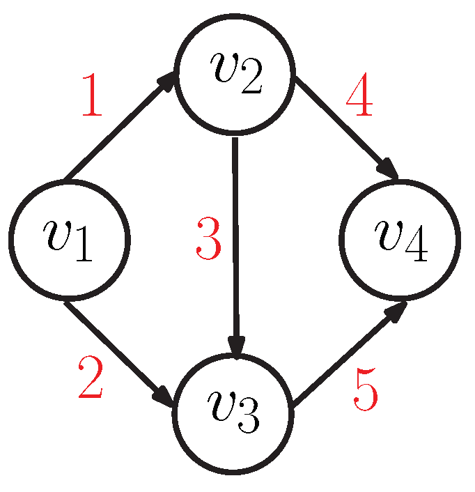
To provide an example, let us consider the activity network in Figure 1 with four vertices and five arcs, that is, modelling the processing of five activities. The execution of the network starts with the parallel processing of activities 1 and 2, since they belong to . As activity 1 is completed, activities 3 and 4 can start since vertex only contains activity 1. Activity 5 can start only if both 2 and 3 have been completed, because contains 2 and 3. Finally, when activities 4 and 5 are completed, the entire network is also completed because vertex does not have any outgoing arc.
Because of the assumptions described above, the dynamics of an activity network can be described by a discrete-state stochastic process whose state corresponds to a vector where each entry , refers to an activity and can assume the values Pending (P), Running (R), and Terminated (T). Entry is equal to P if activity i is waiting for its predecessors to complete and be allowed to start; it is equal to R if activity i is being executed; finally, it is equal to T if activity i has been completed.
The execution of the activities in the network can be modeled through a sequence of states whose transitions are triggered by the completion of a single activity and the number of transitions that departs from a state is always equal to the number of activities that are running in . Let be an indicator function that is equal to one when a transition between a state and a state is possible by means of the termination of the ith activity. Then, we have:
where is a function that returns the set of activities that have to be completed to start activity j but are not yet finished in state . The condition in Equation (1) consists of two terms. The first term, , refers to the activity that causes the transition, therefore activity i must be running in and it must be finished in state . The second term refers to all the other activities defining two possible compatible scenarios. The first one, , refers to activities not changing their status moving from to , that is, running activities keep running while completed activities remain completed. Nevertheless, the start of some activities could be triggered by the completion of activity i, hence, states that there could be an activity j moving from state P to R, but this is possible only if activity i was the only one blocking the start of activity j.
The state transition graph of the stochastic process can be generated based on the conditions in (1). Specifically, starting from an initial state where all the activities are pending but those in , all the possible states can be generated enumerating the completion of each of the running activities, one at time. As all the states have been generated, the procedure necessarily reaches the ending state where all activities are terminated and stop.
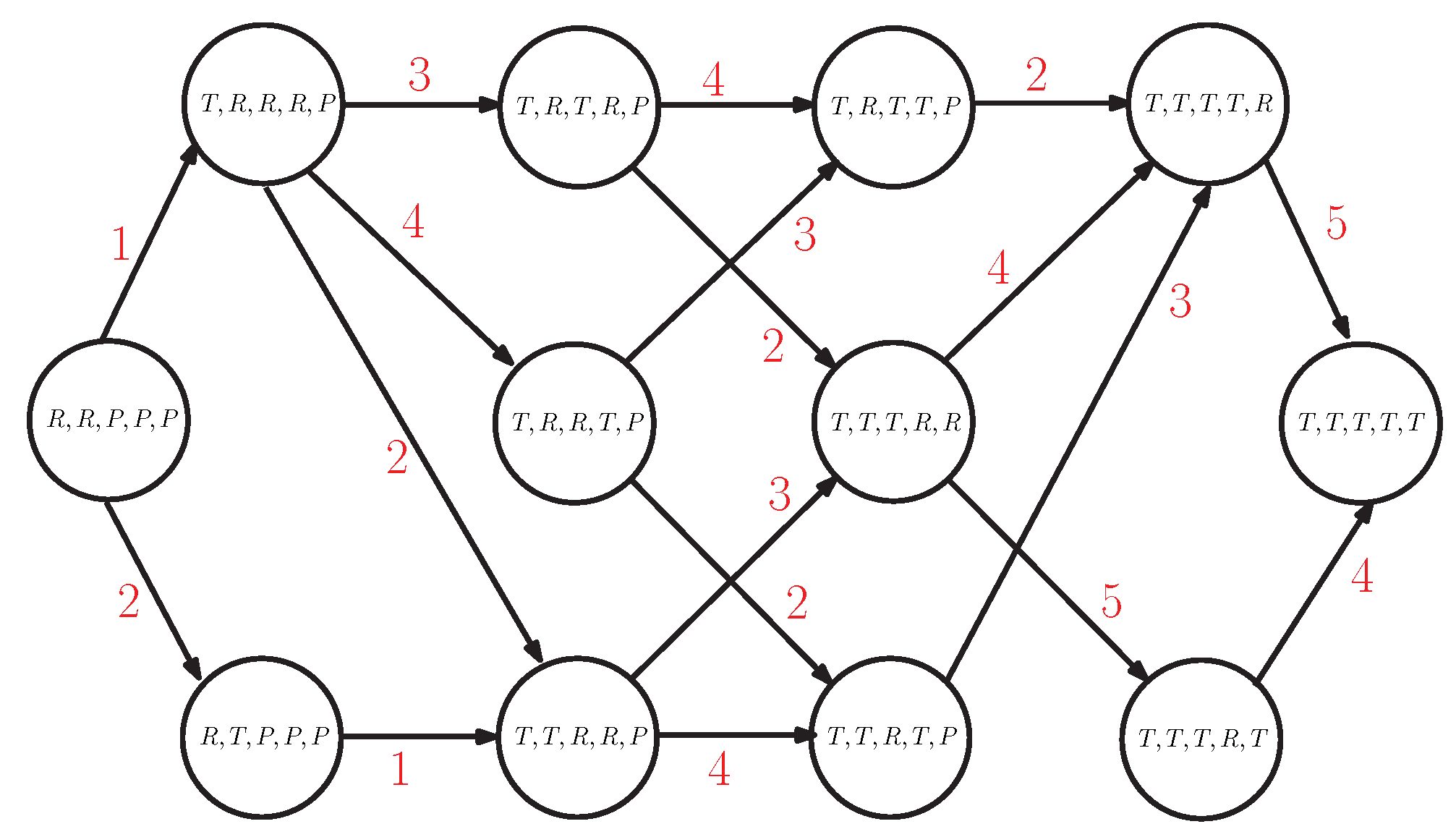
Figure 2 provides an example of the state transition graph for the network in Figure 1. Within each node, the status of the system is defined, for example, the node on the right is the starting node where activities 1 and 2 are running, while the others are pending, that is, . The labels on the arcs indicate the activity, hence, the arc labeled with 1 connects the state with the one representing the state of the system when activity 1 has been completed; that is, activity 4 and 5 can start and the new state is labeled as . The last state on the right is the absorbing one, where all the activities are completed, .
The state transition graph in Figure 2 has some properties: (i) it contains all the possible paths between the initial state and an absorbing one where all the activities are completed; (ii) the length of these paths is constant and equal to K because each of these paths represent a different ordering for the completion of the activities in the network; (iii) the graph does not contain cycles and all its states are transient, except for the absorbing one .
As claimed at the beginning of the paragraph, under the assumption that the durations of the activities are modelled with exponential distributions, that is, , , where is the average time of the activity and the activity network is a MAN. The state transition graph in Figure 2 is the support for the definition of a CTMC whose dynamics are described by a set of ordinary differential equations with cardinality equal to the number of states composing the process.
Assuming to be the probability to find the process in state at time t, each equation has the following structure:
Assuming that all the state probabilities are collected in a vector and all the transitions are grouped in an infinitesimal generator matrix Q, the solution of the ODE system described in Equation (2) is given by and the entry of that corresponds to contains the cumulative distribution of the time to absorption of the CTMC, that is, the distribution of the makespan of the network of activities. The term is the initial probability vector whose entries are all equal to zero, but the one referring to the initial state whose probability is 1.0. The function is the matrix exponential, whose computation is a common problem whose solution can take advantage of a wide range of efficient and numerically safe methods (e.g., [34]).
As an example, Table 1 reports the infinitesimal generator for the model in Figure 1. The infinitesimal generator is a matrix describing the state transition graph in Figure 2. For each possible transition from a state to another, the infinitesimal generator contains the rate of the activity causing the transition. The values on the diagonal, on the contrary, correspond to the sum of all the rates going out from the state called intensity. The initial activities are 1 and 2, thus, the initial state is , with , since it is the only nonzero entry of .
Although it provides a considerable advantage in terms of computation, the restriction to exponentially distributed activity durations represents a limiting hypothesis, specifically in the application to real industrial processes and, hence, to scheduling.
In the following, we present an extension of a classical MAN taking advantage of methods available for CTMCs by using a class of distributions able to approximate general distributions with arbitrary accuracy.
4. Phase-Type Distributions
In the field of Markov models, phase-type (PH) distributions are widely used to provide an approximation of a general distribution. Basically, a set of inter-related exponential delays are put together to approximate a general distribution. Formally, a continuous-time PH distribution is the distribution of the time to absorption of a CTMC, and its order is given by the number of the contained transient states. Consequently, the PH distribution is defined through a vector , providing the initial probabilities of the transient states and a matrix T containing the intensities of the transitions among the transient states.
The cumulative distribution function is given by
whereas the probability density function corresponds to
The i-th moment of a PH distribution is equal to
where denotes a column vector of ones of the same dimension of the T.
PH distributions provide a way to fit a general distribution with a certain degree of accuracy. It must be noted that a MAN can be seen as a PH distribution; in fact, the time to absorption in a MAN, usually not exponentially distributed, is represented through a structure of exponential delays (the execution of each activity) with mutual interactions (precedence relations among the activities).
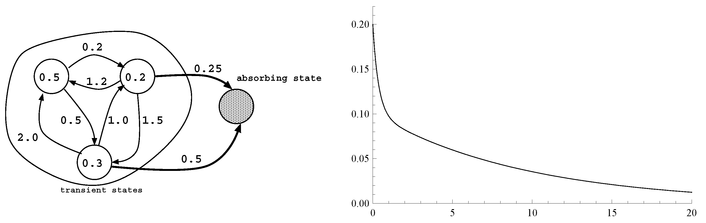
As an example, let us consider the CTMC in Figure 3 with four states, three transient and one absorbing, whose initial probabilities and infinitesimal generator are:
The entries of must sum up to one, while the sum of the elements in a row of Q must be equal to zero. Thus, the representation for this PH distribution is redundant. A non-redundant representation can be obtained by considering the transient states only, resulting in:
The structure of the generator T determines the class of the PH distribution and its capability to catch the moments of the distribution to approximate [35,36]. An exhaustive description of the possible classes of PH distributions is beyond the scope of this paper. Nevertheless, it is important to point out that the method presented in the next section supports the use of any class PH distribution without limitations.
5. Markov Activity Networks Enhanced with PH Distributions
In this section, we extend the formalism of MAN to embed the use of PH distributions and cope with non-exponential durations of the activities, while keeping the advantages provided by a CTMC model. We assume that the processing time of an activity i is distributed according to a PH distribution with representation , . Additionally, in this case we assume that durations of the activities are mutually independent.
Due to this hypothesis, the structure of the CTMC modeling the execution of the activities is more complicated, because every state of the original model has to be expanded to consider the sub-states related to the PH model, that is, the aging of the activities in process. Thus, the execution of the activities progresses according to two levels: a macro level characterized by the completion of the activities, triggering the start of the execution of new ones; and the progress among the phases of the PH distribution of each activity during its execution.
The dynamics of the process modeling the execution of the MAN is still governed by an ODE system, but the probability of a single state evolves over time, according to the following differential equation:
where and are matrices describing the transitions within a single state and between two states, respectively. In particular, describes the aging of the PH distributions within state , that is, the parallel execution of activities that are being processed in . In more detail:
where ⨁ is the Kronecker sum operator. On the contrary, matrix describes the dynamics triggered by the completion of an activity i and the consequent transition from state to state . Thus, the matrix embeds the dynamics related to:
- The completion of the activity that caused the transition from to ;
- The memory of the states within the PH for the activities that were running in state and will continue to run in ;
- The start of activities triggered by the completion of activity i defined by precedence relations.
In formulas, this corresponds to:
In Equation (8), ⨂ denotes the Kronecker product operator iterated over all the activities in , and is an identity matrix whose size is equal to the order of the PH distribution associated with activity j, and .
The value of in Equation (8) is different according to the status of the considered activity j in and . If , then activity j is the one that has been completed, and is a vector that contains the “finishing” intensities of the PH distribution associated to activity j.
If activity j is starting later due to the completion of activity i, then coincides with the initial vector of the PH distribution ().
If activity j is running in both and , is equal to the identity matrix .
Finally, if activity j is not active in both and , is equal to 1 and has no impact in the Kronecker product.
The initial probability vector of the ODE system requires some reformulations. In fact, it is now composed of multiple blocks corresponding to phases of the PH distributions, and it must take into consideration the fact that each of them has its own initial vector.
Let us assume that is the initial state; then is equal to and coincides with the nonzero entries of the initial vector .
The infinitesimal generator for the network in Figure 1, where PH distributions are used for all the activities, is reported in Table 2. The structure of the matrix is the same as the exponential case (Table 1). However, the matrix contains sub-matrices instead of scalar values. Matrices D are placed on the diagonal, since they describe the dynamics within a given state, where one or more activities are in progress. Matrices O are placed out of the diagonal, describing the dynamics of the transitions between states.
If we consider state , , modeling the superposition of the PH distributions active in that state, that is, the ones associated to activities 1 and 2. Additionally, if we consider the transition between state and , this is caused by the completion of activity 1, but it must also keep the memory of the PH distribution of activity 2 (the associated sub-states remain the same during the transition). Moreover, the completion of activity i also triggers the start of activities 3 and 4. Thus, , with containing the rates characterizing the completion of activity 1, keeps the memory of activity 2; and initialize the PH distributions of activities 3 and 4. The initial activities for the whole network are 1 and 2, thus, . Finally, it is important to point out that the Kronecker sum and the Kronecker product do not have the commutative property, hence, the order of the operations must be preserved.
6. A Kroncker Algebra Approach for a Markov Activity Network with PH Distributions
There are several reasons supporting the use of a structured approach based on Kronecker algebra for the formal description of a Markov activity network enhanced through PH distributions. The first one, as stated in [37] with respect to matrix-geometric solutions for stochastic models, is to ensure that the models are in the best and most natural form for numerical computation. For this reason, although unstructured approaches have been proposed to expand the state space of a CTMC with additional states to mimic the behaviour of PH distributions [4,5], these are practicable only for a subset of PH distributions having a simple structure, such as the Coxian, the Erlang, or the Hyper-Exponential.
These approaches also quickly become unfeasible for certain classes of acyclic phase-types as, for instance, the Hyper-Erlang, which corresponds to a mixture of Erlang distributions having a different number of phases. Due to their structure, the Hyper-Erlang is extremely sparse and the tracking of each chain of states is not straightforward, already with a small number of phases. Despite this, their use is fundamental for the fitting of empirical data which are often characterized by irregular shapes and multi-modalities. These situations are often troublesome for the approaches based on moment-matching, because: (i) the moments might not satisfy the bounds of the PH class; (ii) a proper characterization of the shape of the distribution might be preferable to an exact estimation of the first N moments (see [38] for a detailed description of these cases).
Although such cases may seem pure theoretical speculations, their relevance in the modeling of real industrial cases is rather common. An example is manually executed activities, whose duration, as long as the execution goes smoothly, can be easily modeled through simple distributions. On the contrary, the occurrence of possible problems in their execution causes the duration to increase, and the probability distribution fitting the processing times is likely to be multi-modal. In such cases, simply fitting the first two (or three) moments does not provide a reasonable approximation, and different classes of PH distributions could be needed.
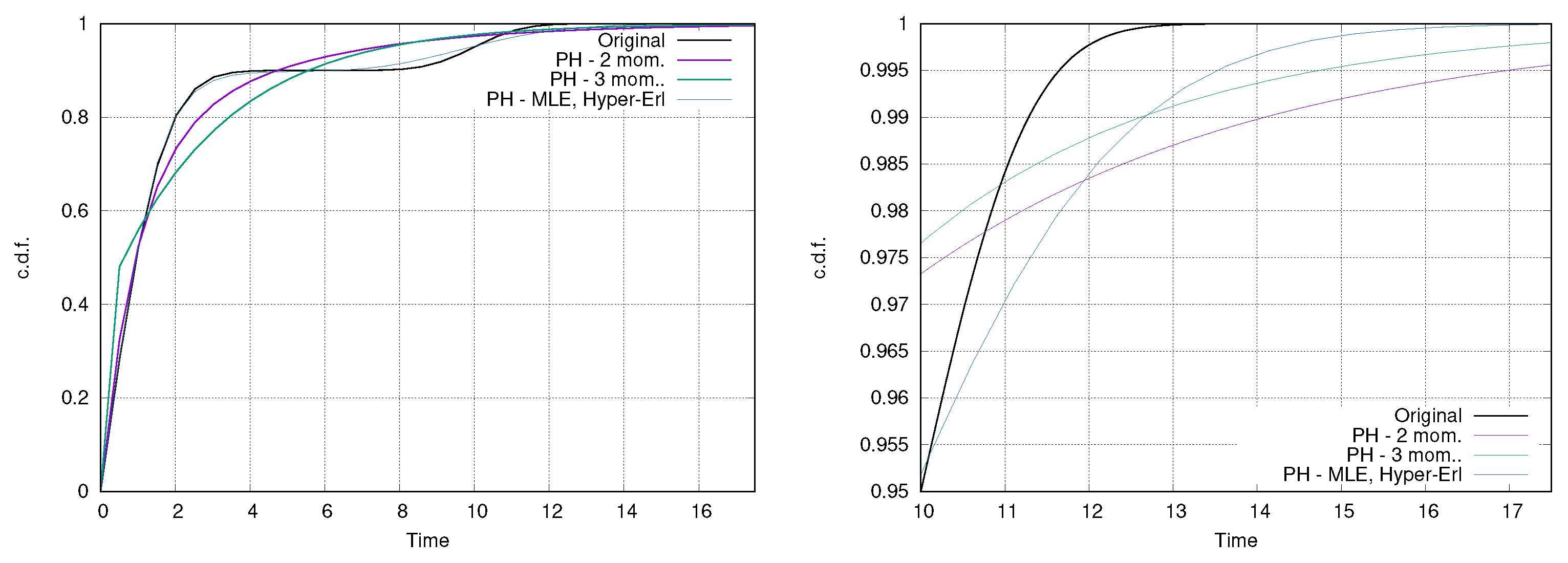
Figure 4 provides a graphical example of a case where moment-based approaches exploiting an acyclic PH are outperformed by a different fitting approach, namely a Hyper-Erlang distribution obtained through Hyper-* [39], a tool that couples clustering approaches with methods for the fitting of phase-type distributions. Figure 4 shows how the moment-based approaches fail in representing the bi-modality of the distribution, whereas the Hyper-Erlang is able to approximate the original distribution with good accuracy. Moment-based methods perform slightly better on the tail of the distribution where they are able to outperform the Hyper-Erlang between 10 and 12. The matching of three moments generates much smaller phase-types than the one provided by Hyper-* (in the case presented, 2 against 29 phases), but does not provide an adequate approximation. Specifically, the phases of the Hyper-Erlang are organized in three Erlang distributions: the first is made up of three phases, with = 2.301 and a probability to be chosen equal to ≈45%; the second with a single phase, and probability ≈0.44%; and the last one composed of 25 phases, with and probability ≈10%. Since with this class of fitting methods (e.g., [39]) the structure of the Hyper-Erlang (in terms of number of branches and length of each path) cannot be foreseen, it is not straightforward to enhance the Markov activity network with these classes of PH distributions by simply expanding the state space of the CTMC through unstructured approaches.
In addition, unstructured approaches become even more impractical when coping with cyclic distributions, that is, creating loops within the states of the CTMC. The use of cyclic PH distributions in practical scheduling problems is justified by concrete requirements. The first one is that, although the class of acyclic phase types is able to represent any cyclic phase-type, there is no guarantee on the finiteness of the number of phases. Hence, a cyclic phase-type might be able to approximate a distribution in a more compact way. This applies for specific classes of distributions, for example, mixtures of monocyclic phase-types (see [40]). Algorithms for the fitting of cyclic phase-types exist and are currently being used; for example, the Butools library provides a method for the transformation of a matrix exponential distribution in a monocyclic phase-type [33].
Another notable reason is that cyclic phase-types are massively used in the context of fault tolerance systems, where mechanisms for restarting, rejuvenation, and check pointing are implemented to model the execution of specific classes of processes often restarted by a controller, when their duration exceeds a certain threshold, or when a risk of stalling [41] arises. These models also allow the use of Kronecker algebra to combine two or more simple dynamics to represent a more complex phenomenon, for example, the failure modes of a machine tool in isolation together with the degradation of a machine tool during the execution of a machining process [42].
Finally, the last argument supporting a structured approach based on Kronecker algebra is that it decouples the exploration of the state space from the PH distribution of each activity. Therefore, the selection of a proper PH approximation for certain activities does not require the redefinition of the whole state space, but only involves those states where the modifications have an impact.
In conclusion, the use of a structured approach to embed PH distributions into activity networks is preferable to unstructured approaches imposing limitations on the class of approximating distributions, as well as failing to provide support for efficient calculation.
7. Testing
This section provides a set of experiments to test the model described in Section 3, as well as an assessment of the degree of approximation entailed by the use of PH distributions with a limited number of phases. The goal is to demonstrate the accuracy achievable in the estimation of the distribution of the makespan with generally distributed durations of the activities modeled with PH distributions. In addition, results related to the required computation time are reported.
The testing phase is organized in three parts. The first one focuses on the evaluation of the impact of a single PH distribution in the activity network in Figure 1, by assessing the accuracy of the fitting for a small activity network. The second one takes into consideration a more general case, where all the activities are non-exponential and, thus, approximated through PH distributions. The aim is to show how the errors associated to each activity have an impact on the estimation of the makespan. Finally, the third part reports the results obtained by using the proposed approach on a set of 150 networks, randomly selected from the PSPLIB set of instances [43]. This part also reports a more detailed analysis of the performance of the approach in terms of computational effort, with respect to the number of states composing the underlying Markov chain. All the experiments have been carried out using a JAVA code implementing both the numerical methods for the analysis of the activity networks using PH approximations and a Monte Carlo simulator to provide an exact estimation of the makespan distribution. The fitting of PH distributions has been operated using the software packages Butools 2.0 [33] and Mathematica 11.0 (other commercial tools like Matlab, and free software like Octave or Python could also be easily used to develop the approach).
7.1. Activity Network with a Single PH Distributed Activity Duration
To analyze the impact of a single PH distribution in a network, we consider the one in Figure 1. Three experiments have been carried out with different classes of distributions. Each experiment is organized in two steps:
- A PH distribution is fitted to approximate the general distribution;
- The resulting PH distribution is plugged into the activity network.
The first step takes advantage of two fitting methods, although any fitting method able to generate a PH distribution can be used. The first one, described in [36], is based on MLE and takes as input a set of data-points and the desired number of phases. The data-points are fitted into a PH distribution corresponding to a hyper-Erlang distribution having the specified number of phases. The second method, described in ([31]), is based on moment-matching. It considers up to three moments and returns a PH distribution with an arbitrary number of phases matching the moments. Both the methods are available in the Butools library. Alternative tools for the fitting of PH distributions are implemented in the software packages PH-fit [32] and G-Fit [36].
The second step addresses the activity network in Figure 1, assuming that all the activities but 3 are distributed according to the Erlang-5 distribution. Since this distribution belongs to the family of PH distributions, its PH representation is exact. On the contrary, the duration of activity 3 is assumed to be generally distributed and approximated through the fitting of a PH distribution according to what is described for the first step. Hence, the durations of activity 1, 2, 4 and 5 are modeled exactly, while an approximation can exist for activity 3. This approximation is the only source of error.
The decision to perform the testing on activity 3 is aimed at stressing the accuracy of the model. In fact, activity 3 connects the two paths 1–4 and 2–5 (Figure 1). To make the impact of the activities on the makespan uniform, their mean duration was set to 5.
The experiments have been carried out considering three different classes of distributions for activity 3:
- Normal: It represents the ideal scenario for PH approximation because it is continuous and light-tailed on both sides;
- Log-Normal: It is a more challenging scenario because of heavy tails;
- Uniform: It represents the more difficult case, because PH distributions cannot model a distribution with finite support. Hence, a higher number of phases will be needed to reach a reasonable approximation.
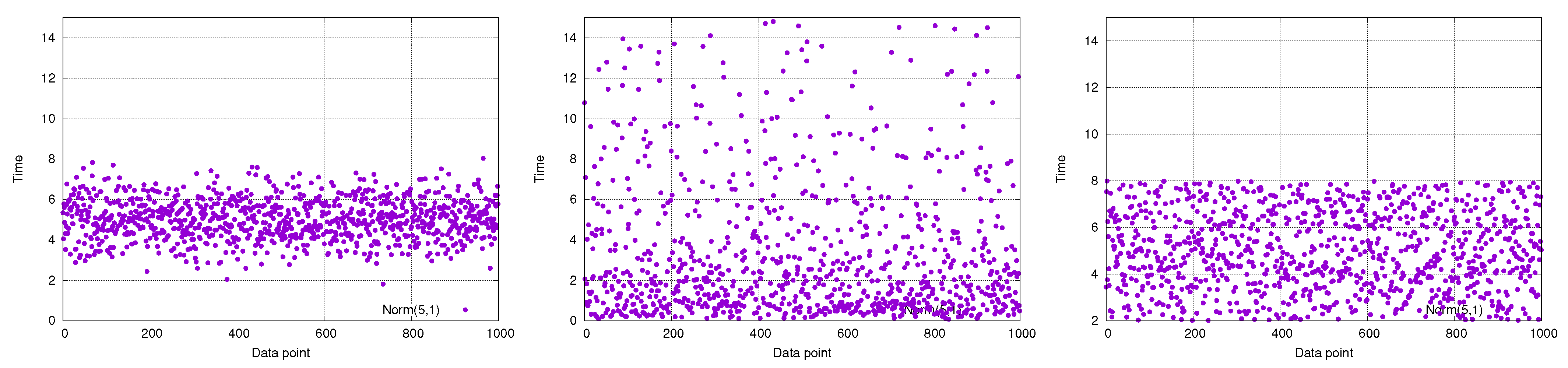
Figure 5 provides a graphical representation of the differences between the distributions used in the three scenarios with each plot showing 1000 data-points. It is possible to notice that points related to a normal distribution are centered around 5 and their frequency decades with the distance from the average. On the contrary, points drawn from the log-normal are sparser and can be found at high values, whereas those drawn from the uniform distribution are equally distributed all along the interval.
For this set of experiments, both the Monte Carlo simulations and the CTMC calculations required less than a second to be performed. Confidence intervals are not provided because more than 100,000 runs have been computed for the Monte Carlo approach; hence, the intervals are tight enough not to be visualized.
7.1.1. PH Approximation for a Normally Distributed Activity
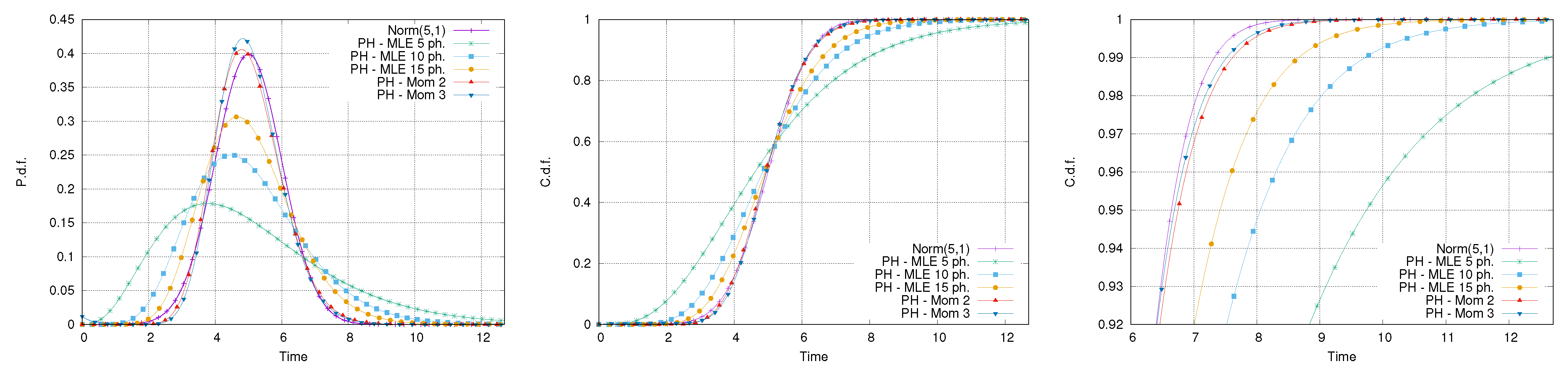
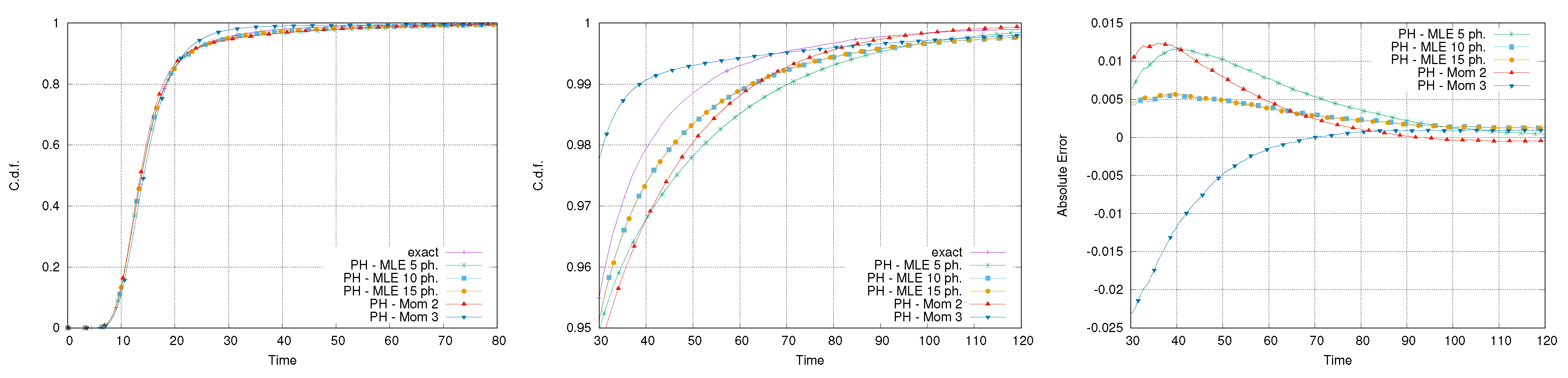
The first set of experiments addresses the use of PH to fit a normal distribution, with a mean equal to 5 and a coefficient of variation equal to 0.2. A very small coefficient of variation has been used to mimic an industrial scenario where activities have a high level of formalization and, thus, are usually characterized by a small variation. This choice also guarantees the absence of negative values, impossible for a time span, during the fitting phase. Five different fitting approaches have been performed: the first three using the MLE method with a number of phases equal to 5, 10, and 15, respectively; the fourth and the fifth using the moment-based approach by matching the first two and the first three moments. The PHs generated through the moment-based approach had orders equal to 25 and 28, respectively.
Figure 6 reports the comparison between the original normal distribution and the fitted PH ones. It is possible to notice that only the distributions fitted using the moment-matching method have a Gaussian-like shape, whereas the other PH distributions underestimate the peak and are far from being symmetric. This is a consequence of the small coefficient of variation used, requiring a high number of phases to be fitted. Despite this, observing the right tail of the distribution, it is possible to notice that the absolute error for the 95th and 99th percentile, obtained using the PH approximation with 15 phases, is rather small, that is, about 1 time unit.
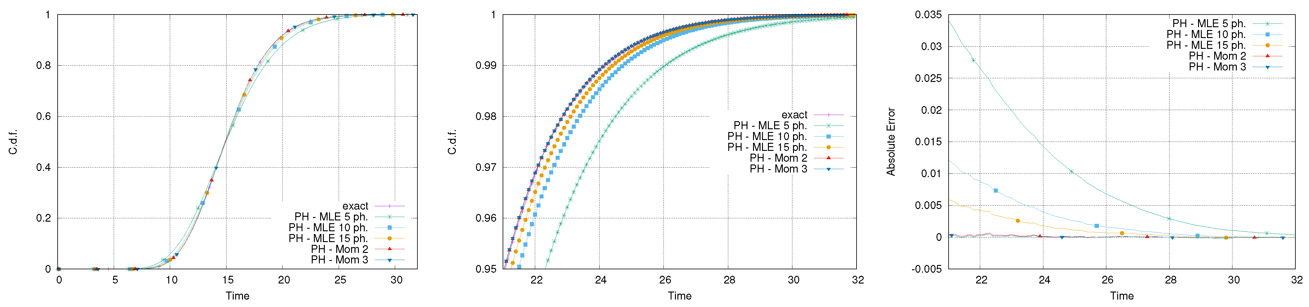
Figure 7 reports the exact and PH-approximated distributions of the makespan for the network of activities in Figure 1. It can be observed that all the approximated makespans are able to provide a reasonable approximation. This is particularly evident by observing the right tail of the distribution, where the absolute error remains below in all the cases.
7.1.2. PH Approximation for a Log-Normal-Distributed Activity
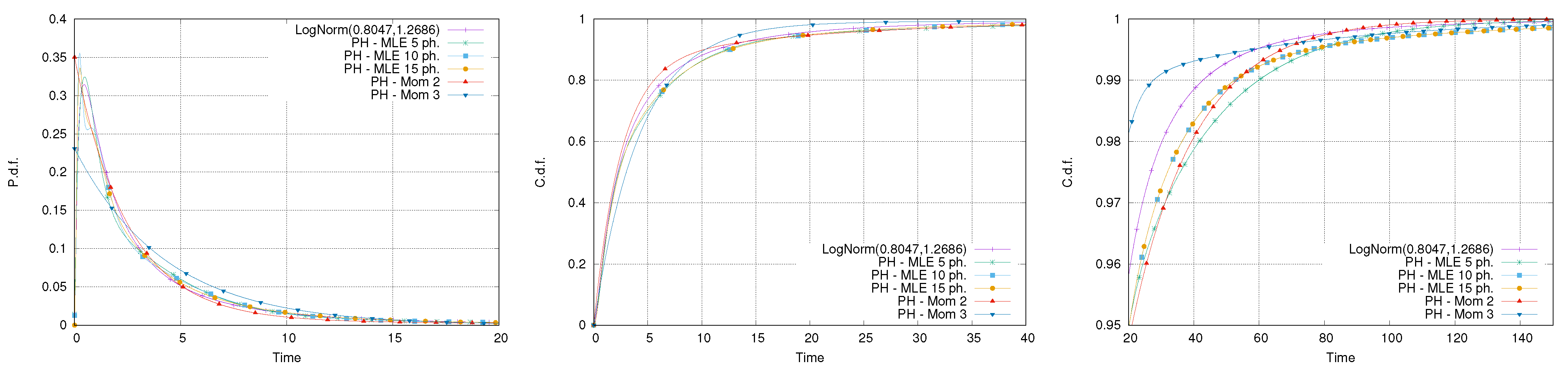
The second set of experiments considers a log-normal distribution with parameters and . This corresponds to a mean equal to 5 and coefficient of variation of 2. The same fitting approaches of the previous case have been used and, in this case, the moment-based approach was able to match the first three moments by using only two phases.
Figure 8 reports the result of the fitting. It is possible to notice that the worst approximation is provided by the PH distribution that matches three moments. This result is counter-intuitive because, at least in principle, the distribution matching the first three moments should provide a better approximation than the distribution that matches only the first two.
However, this phenomenon might occur when using a fitting method that only considers moment-matching, because it does not guarantee any accuracy with respect to the shape of the distribution. Therefore, for heavy-tailed distributions, matching additional moments is not likely to improve the accuracy of the fitting, particularly for small quantiles. In fact, the fitting matching three moments in this case provides an accurate approximation for extremely high values of the quantiles only.
Figure 9 reports the exact and PH-approximated distributions of the makespan for the network of activities in Figure 1. The plots confirm the errors highlighted in Figure 8 for the fitting. Specifically, referring to the tail of the distribution of the makespan, this was partly expected. The Erlang-5, the PH distributions obtained using five phases, has a low coefficient of variation in comparison with the log-normal, therefore, the propagation of the error significantly affects the accuracy in the estimation of the distribution of the makespan. Despite this, the absolute error for all the approximated distributions of the makespans stays below , with respect to the tail of the distribution (Figure 8, right).
7.1.3. PH Approximation for a Uniform Distribution
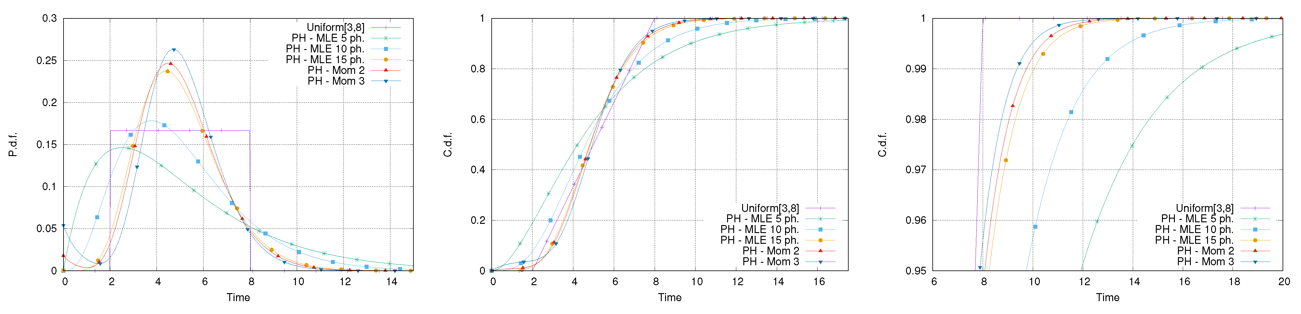
The third set of experiments considers a uniform distribution in the interval . In this case, there is no chance for a finite number of phases to be able to represent the finite support of the uniform distribution. The moment-based approach requires nine phases to match the first two moments and 12 to match the first three. The impact of this limitation for PH distributions is clear by observing Figure 10 reporting the result of the fitting. It is possible to notice that the pdf of the approximating PH distributions tends to be bell-shaped and trespasses the limited domain of the uniform distribution both in the right and left tails. Additionally, the shape of the tail is overestimated by all the approximating PH distributions (Figure 10, right).
Figure 11 shows the comparison between the exact and approximated distribution of the makespan of the activity network in Figure 1 showing that the overall error reduces in comparison with the one related to activity 3 only. In particular, while the PH distribution of order 5 demonstrates an error greater than in the tail of the distribution, the other approximating distributions have an error that stays below and becomes almost zero near the 99th percentile.
7.2. PH Approximation for All the Activities in the Network
In this section, we hypothesize a general distribution for all the activities in the network, with the aim to show that the accuracy in the estimation of the makespan is reasonable even with a large number of approximated distributions. For this test, we used a 30-job instance from the PSPLIB set of instances [43]. Since the repository only contains activity networks with deterministic durations, a distribution and a coefficient of variation have been randomly sampled for each activity, whereas the mean value has been set equal to the original deterministic duration. Two classes of distributions have been considered: log-normal and half-normal, with each activity having the same probability to be distributed as one or the other. The coefficients of variation have been assigned in a similar way, by sampling among three possible values: 0.5, 1, and 1.5.
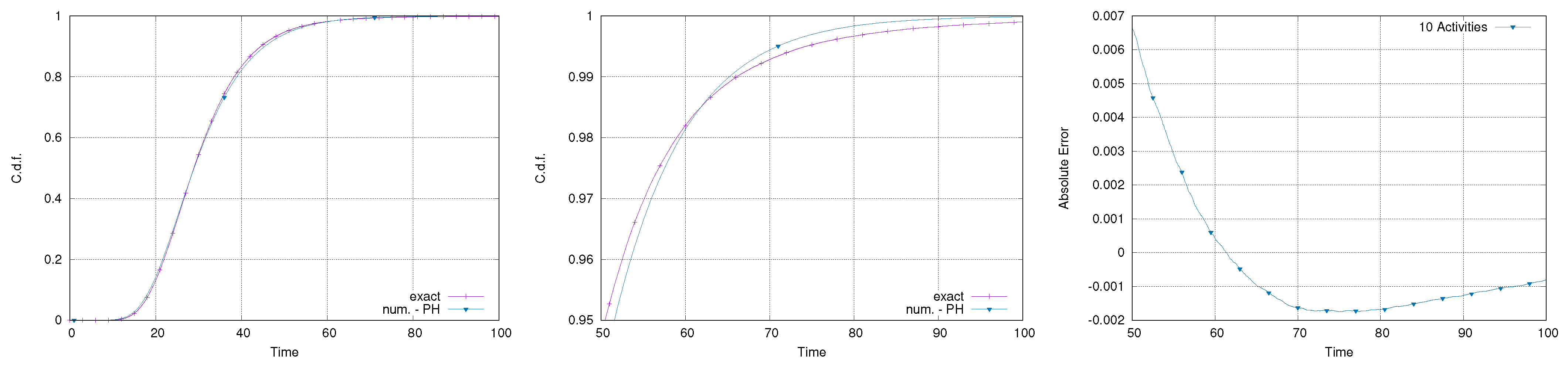
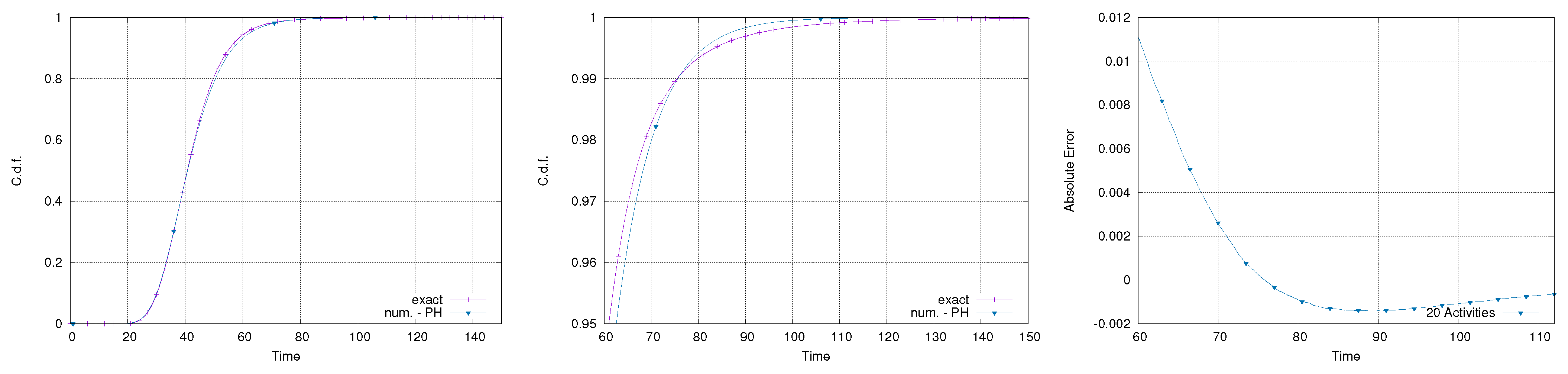
The 32 activities in the network, together with their distributions, have been fitted by matching the first two moments. All the fittings required, at most, four phases to match the moments. Then, three sub-models have been considered in order to analyze the approximation error as the number of approximated distributions increases. Specifically, within the same network, subsets containing the first 5, 10, and 20 activities have been considered.
The structure of the network and its distributions are reported in Table 3. Horizontal lines delimit the considered subsets.
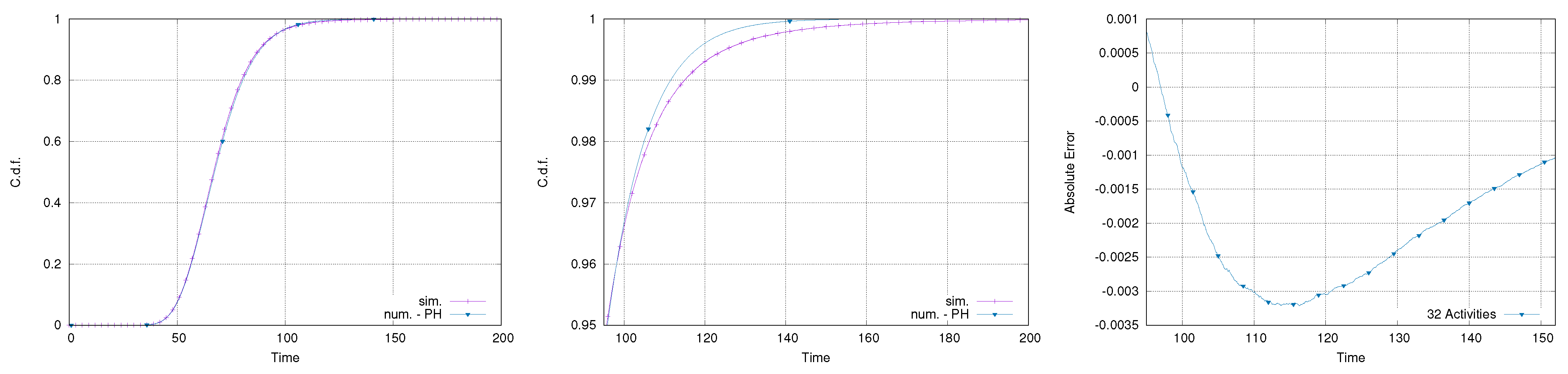
The four networks with an increasing number of activities have also been analyzed using a Monte Carlo simulation, to provide a reference distribution to be considered as the real one. Table 4 summarizes the experiments, showing that the state space of the CTMC grows very fast and the number of transitions increases even faster. Despite this, for a network consisting of up to 20 activities, the numerical solution requires less time than performing 100,000 samples for the Monte Carlo simulation.
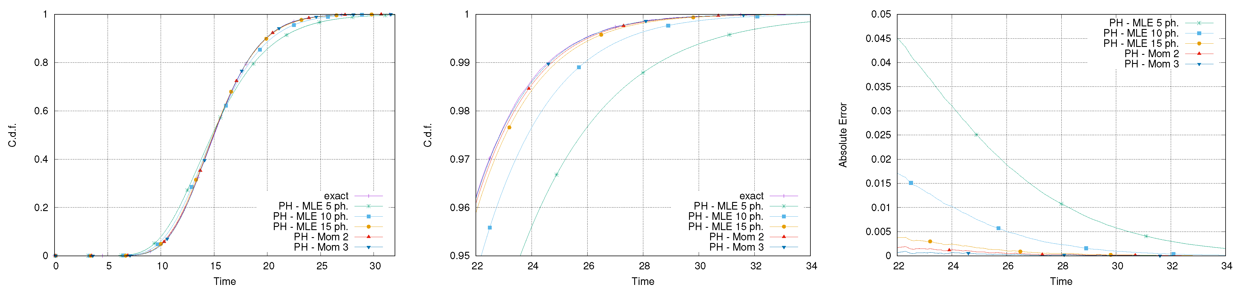
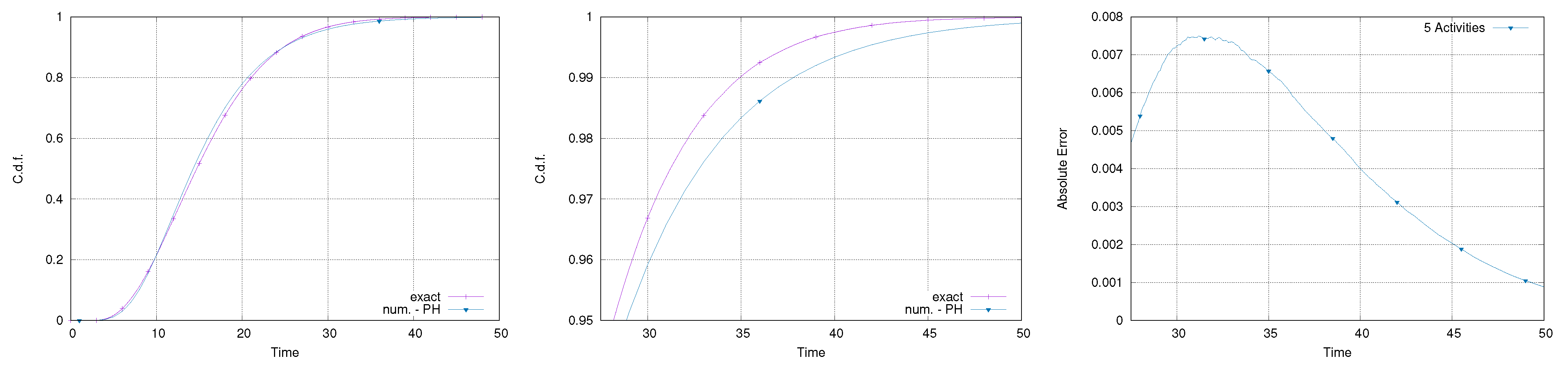
Figure 12, Figure 13, Figure 14 and Figure 15 report the results of the calculation of the makespan for the four models considered. All the comparisons show good accuracy and an error on the percentiles that rarely exceeds . Specifically, it is relevant to notice that the error does not increase with the number of activities. Although there is no guarantee for these results to represent a general behavior, it is important to point out that all the fittings have been done automatically, without any specific selection or tuning of the fitting method.
7.3. Test on a Set of Activity Networks
The described approach has been tested on multiple networks of activities obtained by randomly selecting a set of 150 from the instances in the PSPLIB [43]. The structure of the networks has been considered as given, while the randomness in the duration of the activities has been introduced using the same approach described in Table 3. Hence, a PH distribution has been fitted for each activity in the network by matching the first two moments. The fitting of the activity distributions has been done in negligible time. In fact each activity required 0.017 s, on average, to find the approximating PH type.
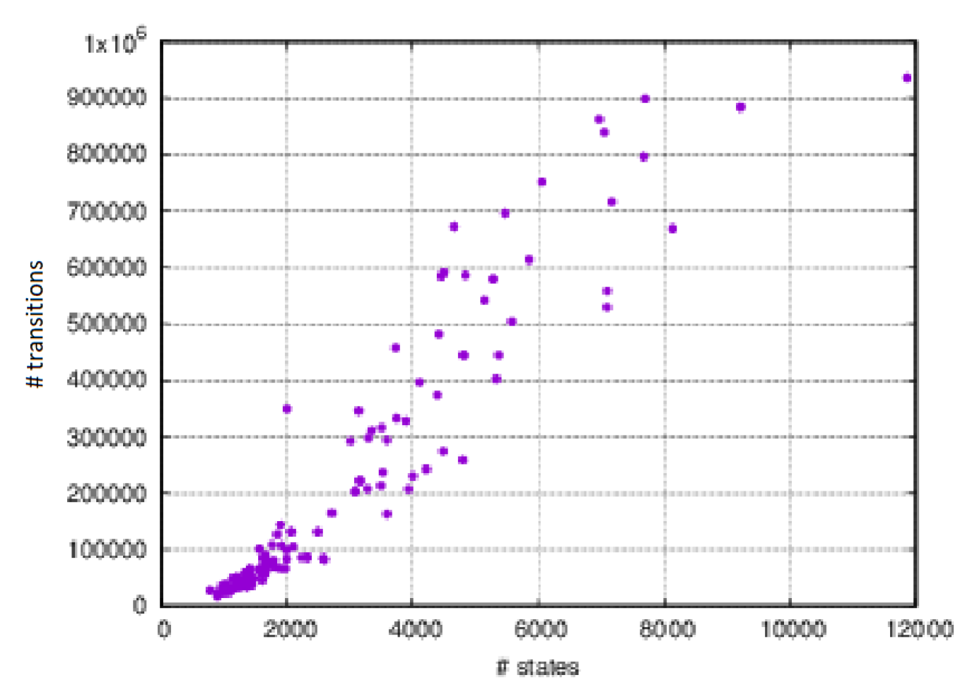
Figure 16 provides a quick glimpse of the heterogeneity of the networks considered in the experiment, by showing a clear direct correlation between the overall number of transitions and the number of states for each network.
However, the higher the number of states composing the CTMC, the more variable the number of transitions in the model. This is due to the fact that the number of transitions heavily depends on the level of concurrency in the network, that is, the number of activities that are in execution in each state. A network having many activities and, consequently, many states, has a higher probability of having multiple activities in execution at the same time. If this number is high, the number of transitions is high as well. As a consequence, the number of PH distributions enabled at the same time in the states, and the consequent number of transitions, is less variable among the different instances. A summary of the networks used for the experiments is reported in Table 5, providing information in terms of the number of states composing the CTMC and the number of transitions. It is possible to observe that the average number of states is equal to 2763.73, with a minimum of 779 states and a maximum of 11,858. On the contrary, the average number of transitions is equal to 207,343.59, with a maximum of 935,440 and a minimum of 17,298.
In order to quantify the error introduced by the approximation using PH distributions, we consider the average Kullback–Leibler divergence (KL) of the network, also called average entropy, defined as
where is the probability density function (pdf) of the exact distribution for activity i, is the pdf of the approximated PH distribution, and K is the total number of activities in the network and the integral is operated on the duration of each activity. If the durations of the activities in the network are well-approximated by the PH distributions, is close to zero.
Table 5 also reports the value of the average entropy corresponding to 0.0359. Being the value rather close to zero, we can conclude that the PH distributions approximate the general distributions with good accuracy, despite the fact that only the first two moments are matched.
Table 6 compares the time required to compute the quantile of the distribution of the time to absorption of the CTMC with PH distributions, that is, the distribution of the makespan for the network of activities. This performance is compared with the one obtained executing a Monte Carlo simulation with one million samples from the original distributions.
It is possible to observe that the Monte Carlo simulation is, on average, faster than the numerical solution. The good performance of Monte Carlo simulation is due to:
- Large networks requiring a considerable amount of data to be stored in the RAM and slowing down the computation due to the swapping between primary and secondary memory;
- The calculation of the desired percentiles (performed with the bisection method) that increases the computational effort.
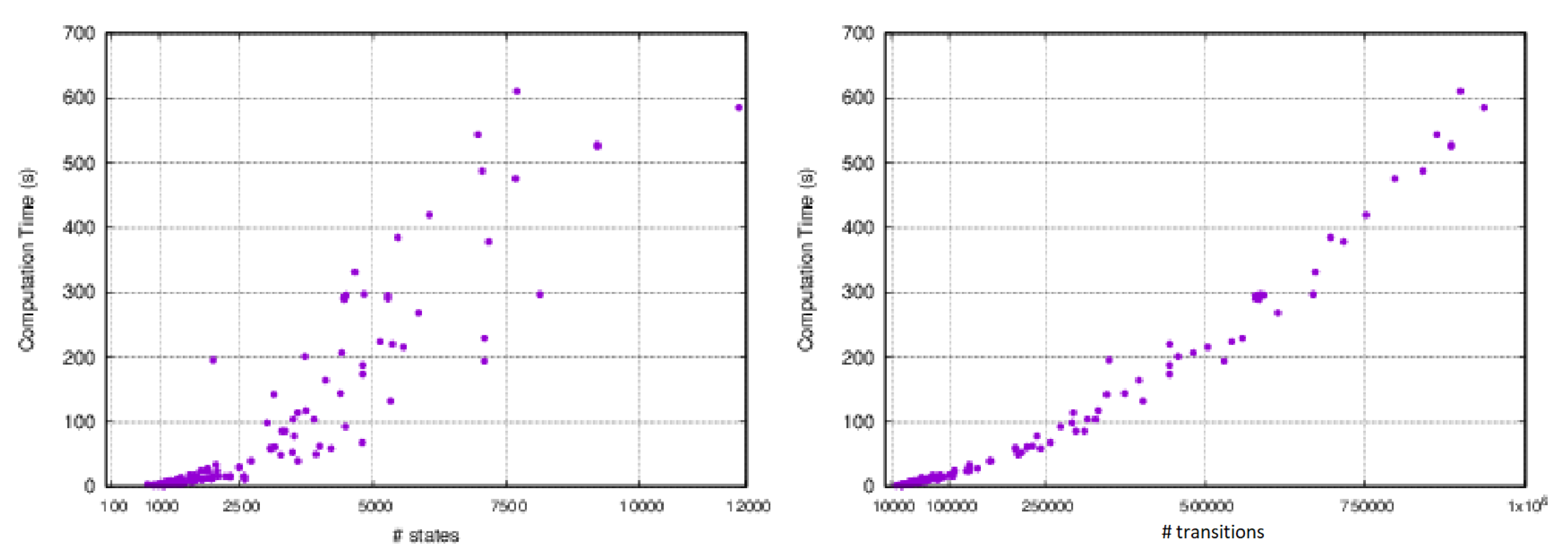
To provide a clearer picture of the overall performance of the approach, Figure 17 shows the computation times for all the experiments in relation to the number of states of the CTMC and the number of transitions. It is clear that the computation time increases exponentially with the size of the problem. Indeed, the Monte Carlo simulation does not suffer from this problem, since the overall complexity is bounded by , where R is the number of simulation runs. Nevertheless, it is important to point out that:
- The CTMC can be solved using more advanced techniques able to reduce the computation time;
- The CTMC defines a model for the execution of the network of activities that can support decomposition approaches, for example, calculating subnets and incorporating the obtained solution or estimation in the comprehensive network.
Finally, Table 7 reports the error in the estimation of the distribution of the makespan using PH distributions for different percentiles. It is possible to notice that the error increases with the considered percentile. At the 90th percentile, the error is, on average , and the confidence interval is , with a minimum of and a maximum of , whereas at the 99th percentile, the error is, on average, with a confidence interval equal to , a minimum of and a maximum of .
8. Conclusions
In this paper, a general approach has been proposed to exploit Markov chains and phase-type distributions to model the execution of a stochastic PERT network with general distributed processing times. A general and concise formulation has been proposed, based on Kronecker algebra, to support the application without any constraint on the class of phase-type distributions allowed.
The motivation for the approach stems from the need to fit real data and use this information in the planning and scheduling of manufacturing operations, overcoming the limitation of a large portion of the literature related to stochastic scheduling, requiring strong hypotheses on the underlying distributions. Coping with real data, characterized by asymmetry, multi-modality, and so forth, PH distributions are a very effective approximation approach also entailing the capability of using Markov activity networks and the associated corpus of approaches.
The proposed formulation also allows to easily change and/or refine the fitting according to the accuracy requirements to keep the computation time in line with the specific needs and without the need of recomputing the whole model from zero.
An analytical description has been provided, as well as experiments on a wide range of test instances. The testing demonstrated good performance both in terms of computation time and accuracy of the approximation, although the computational effort rapidly increases with the dimension of the network and the number of phases used.
Moreover, the algebraic formulation also allows the use of more advanced numerical methods able to evaluate the Markov activity network without the need to explicitly build the whole infinitesimal generator, thus paving the way to more efficient calculation approaches.
Hence, modeling the execution of an activity network through a Markov process and phase-type distributions provides a promising path towards embedding the proposed estimation approach in scheduling algorithms to optimize a function of the makespan distribution, such as an associated risk measure.
Further developments will address advanced calculation methods to speed up the computation time, as well as the exploitation of this method to support stochastic scheduling approaches.
Author Contributions
Conceptualization, M.U.; methodology, A.A., A.H. and M.U.; software, A.A.; writing, A.A., A.H. and M.U. All authors have read and agreed to the published version of the manuscript.
Funding
This research received no external funding.
Institutional Review Board Statement
Not applicable.
Informed Consent Statement
Not applicable.
Data Availability Statement
Not applicable.
Conflicts of Interest
The authors declare no conflict of interest.
References
- Malcolm, D.; Rosenbloom, J.; Clark, C.; Fazar, W. Application of a technique for research and development program evaluation. Oper. Res. 1959, 7, 646–669. [Google Scholar] [CrossRef]
- Kulkarni, V.; Adlakha, V. Markov and Markov-regenerative pert networks. Oper. Res. 1986, 34, 769–781. [Google Scholar] [CrossRef]
- Urgo, M. Stochastic Scheduling with General Distributed Activity Durations Using Markov Activity Networks and Phase-Type Distributions. In Sequencing and Scheduling with Inaccurate Data; Nova Publisher: Hauppauge, NY, USA, 2014. [Google Scholar]
- Elmaghraby, S.; Benmansour, R.; Artiba, A.; Allaoui, H. On The Approximation of Arbitrary Distributions by Phase-Type Distributions. In Proceedings of the 3rd International Conference on Information Systems, Logistics and Supply Chain, Casablanca, Morocco, 13 April 2010. [Google Scholar]
- Creemers, S. Minimizing the expected makespan of a project with stochastic activity durations under resource constraints. J. Sched. 2015, 18, 263–273. [Google Scholar] [CrossRef]
- Creemers, S. Maximizing the expected net present value of a project with phase-type distributed activity durations: An efficient globally optimal solution procedure. Eur. J. Oper. Res. 2018, 267, 16–22. [Google Scholar] [CrossRef] [Green Version]
- Buchholz, P. Structured analysis approaches for large Markov chains. Appl. Numer. Math. 1999, 31, 375–404. [Google Scholar] [CrossRef]
- Buchholz, P.; Kemper, P. Kronecker Based Matrix Representations for Large Markov Models. In Validation of Stochastic Systems: A Guide to Current Research; Baier, C., Haverkort, B.R., Hermanns, H., Katoen, J.P., Siegle, M., Eds.; Springer: Berlin/Heidelberg, Germany, 2004; pp. 256–295. [Google Scholar]
- Ballarini, P.; Horváth, A. Memory Efficient Analysis for a Class of Large Structured Markov Chains: Work in Progress. In Proceedings of the Fourth International ICST Conference on Performance Evaluation Methodologies and Tools, Pisa, Italy, 20–22 October 2009; pp. 21:1–21:4. [Google Scholar]
- Igelmund, G.; Radermacher, F.J. Preselective Strategies for the Optimization of Stochastic Project Networks under Resource Constraints. Networks 1983, 13, 1–28. [Google Scholar] [CrossRef]
- Igelmund, G.; Radermacher, F.J. Algorithmic Approaches to Preselective Strategies for Stochastic Scheduling Problems. Networks 1983, 13, 29–48. [Google Scholar] [CrossRef]
- Radermacher, F.J. Scheduling of Project Networks. Ann. Oper. Res. 1985, 4, 227–252. [Google Scholar] [CrossRef]
- Stork, F. Branch-and-Bound Algorithms for Stochastic Resource-Constrained Project Scheduling; Technical Report; Research Report No. 702/2000; Technische Universität Berlin: Berlin, Germany, 2000. [Google Scholar]
- Tolio, T.; Urgo, M.; Váncza, J. Robust production control against propagation of disruptions. CIRP Ann. Manuf. Technol. 2011, 1, 489–492. [Google Scholar] [CrossRef]
- Radke, A.M.; Tolio, T.; Tseng, M.M.; Urgo, M. A risk management-based evaluation of inventory allocations for make-to-order production. CIRP Ann. Manuf. Technol. 2013, 1, 459–462. [Google Scholar] [CrossRef]
- Urgo, M.; Buergin, J.; Tolio, T.; Lanza, G. Order allocation and sequencing with variable degree of uncertainty in aircraft manufacturing. CIRP Ann. Manuf. Technol. 2018, 67, 431–436. [Google Scholar] [CrossRef]
- Urgo, M.; Váncza, J. A branch-and-bound approach for the single machine maximum lateness stochastic scheduling problem to minimize the value-at-risk. Flex. Serv. Manuf. J. 2018, 31, 472–496. [Google Scholar] [CrossRef] [Green Version]
- Hagstrom, J.N. Computational complexity of PERT problems. Networks 1988, 18, 139–147. [Google Scholar] [CrossRef]
- Kleindorfer, G. Bounding distributions for a stochastic acyclic network. Oper. Res. 1971, 19, 586–601. [Google Scholar] [CrossRef]
- Moehring, R. Scheduling under Uncertainty: Bounding the Makespan Distribution. In Computational Discrete Mathematics; Springer: Berlin/Heidelberg, Germany, 2001; pp. 79–97. [Google Scholar]
- Golenko-Ginsburg, D.; Gonik, A. Stochastic Network Project Scheduling with Non-Consumable Limited Resources. Int. J. Prod. Econ. 1997, 48, 29–37. [Google Scholar] [CrossRef]
- Tsai, Y.W.; Gemmill, D.D. Using Tabu Search to Schedule Activities of Stochastic Resource-Constrained Projects. Eur. J. Oper. Res. 1998, 111, 129–141. [Google Scholar] [CrossRef]
- Buss, A.H.; Rosenblatt, M.J. Activity delay in stochastic project networks. Oper. Res. 1997, 45, 661–677. [Google Scholar] [CrossRef]
- Sobel, M.; Szmerekovsky, J.; Tilson, V. Scheduling projects with stochastic activity duration to maximize expected net present value. Eur. J. Oper. Res. 2009, 198, 697–705. [Google Scholar] [CrossRef]
- Elmaghraby, S.E.; Ramachandra, G. Optimal Resource Allocation in Activity Networks: II. The Stochastic Case; Research Report; NCSU: Raleigh, NC, USA, 2012. [Google Scholar]
- Angius, A.; Horváth, A.; Urgo, M. Analysis of activity networks with phase type distributions by Kronecker algebra. In Proceedings of the 14th International Conference on Project Management and Scheduling (PMS’14), Munich, Germany, 30 March–2 April 2014; pp. 1–5. [Google Scholar]
- Bobbio, A.; Cumani, A. ML estimation of the parameters of a PH distribution in triangular canonical form. Comput. Perform. Eval. 1992, 22, 33–46. [Google Scholar]
- Asmussen, S.; Nerman, O.; Olsson, M. Fitting Phase-Type Distributions via the EM Algorithm. Scand. J. Stat. 1996, 23, 419–441. [Google Scholar]
- Telek, M.; Heindl, A. Matching moments for acyclic discrete and continuous phase-type distributions of second order. Int. J. Simul. Syst. Sci. Technol. 2002, 3, 47–57. [Google Scholar]
- Horváth, G.; Telek, M. A canonical representation of order 3 phase type distributions. Lect. Notes Theor. Comput. Sci. 2007, 4748, 48–62. [Google Scholar]
- Bobbio, A.; Horváth, A.; Telek, M. Matching Three Moments with Minimal Acyclic Phase Type Distributions. Stoch. Model. 2005, 21, 303–326. [Google Scholar] [CrossRef]
- Horváth, A.; Telek, M. PhFit: A General Phase-Type Fitting Tool. In Proceedings of the 12th Performance TOOLS, London, UK, 14–17 April 2002; Volume 2324. [Google Scholar]
- BuTools 2.0. 2018. Available online: http://webspn.hit.bme.hu/~telek/tools/butools (accessed on 1 April 2021).
- Moler, C.; Loan, C.V. Nineteen Dubious Ways to Compute the Exponential of a Matrix, Twenty-Five Years Later. SIAM Rev. 2003, 45, 3–49. [Google Scholar] [CrossRef]
- Horváth, A. Approximating Non-Markovian Behavior by Markovian Models. Ph.D. Thesis, Department of Telecommunications, Budapest University of Technology and Economics, Budapest, Hungary, 2002. [Google Scholar]
- Thummler, A.; Buchholz, P.; Telek, M. A Novel Approach for Phase-Type Fitting with the EM Algorithm. IEEE Trans. Dependable Secur. Comput. 2006, 3, 245–258. [Google Scholar] [CrossRef]
- Neuts, M.F. Matrix-Geometric Solutions in Stochastic Models: An Algorithmic Approachg; Dover: Mineola, NY, USA, 1981. [Google Scholar]
- Angius, A.; Horvath, A.; Halawani, S.M.; Barukab, O.; Ahmad, A.R.; Balbo, G. Constructing Matrix Exponential Distributions by Moments and Behavior around Zero. Math. Probl. Eng. 2014, 2014, 610907. [Google Scholar] [CrossRef]
- Reinecke, P.; Krauß, T.; Wolter, K. Cluster-based fitting of phase-type distributions to empirical data. Comput. Math. Appl. 2012, 64, 3840–3851. [Google Scholar] [CrossRef] [Green Version]
- Mocanu, S.; Commault, C. Sparse representations of phase-type distributions. Commun. Stat. Stoch. Model. 1999, 15, 759–778. [Google Scholar] [CrossRef]
- Wolter, K. Stochastic Models for Fault Tolerance-Restart, Rejuvenation and Checkpointing; Springer: Berlin/Heidelberg, Germany, 2010. [Google Scholar] [CrossRef]
- Angius, A.; Colledani, M.; Yemane, A. Impact of condition based maintenance policies on the service level of multi-stage manufacturing systems. Control Eng. Pract. 2018, 76, 65–78. [Google Scholar] [CrossRef]
- PSPLIB. 2018. Available online: http://www.om-db.wi.tum.de/psplib (accessed on 1 April 2021).
Figure 1.
An activity network.

Figure 2.
State transition graph of the stochastic process for the network of activities in Figure 1.
Figure 2.
State transition graph of the stochastic process for the network of activities in Figure 1.

Figure 3.
Graphical representation of an order of three PH distributions (left) and its probability density function (right).
Figure 3.
Graphical representation of an order of three PH distributions (left) and its probability density function (right).

Figure 4.
Comparison between an empirical distribution fitted by using both moment-based approaches and cluster-based fitting: cdf (left) and tail of the cdf (right).
Figure 4.
Comparison between an empirical distribution fitted by using both moment-based approaches and cluster-based fitting: cdf (left) and tail of the cdf (right).

Figure 5.
Scatter plots of the data-points used for the fitting of the Normal distribution (left), Log-Normal distribution (center), and Uniform distribution (right).
Figure 5.
Scatter plots of the data-points used for the fitting of the Normal distribution (left), Log-Normal distribution (center), and Uniform distribution (right).

Figure 6.
Comparison between the normal distribution with mean 5 and coefficient of variation equal to 0.2 and its fitting by means of PH distributions: pdf (left), cdf (center), and tail of the cdf (right).
Figure 6.
Comparison between the normal distribution with mean 5 and coefficient of variation equal to 0.2 and its fitting by means of PH distributions: pdf (left), cdf (center), and tail of the cdf (right).

Figure 7.
Makespan of the example activity network with the duration of activity 3 following a normal distribution with mean 5 and coefficient of variation equal to 0.2; full (left), only the tail (center), and the tail approximation error (right).
Figure 7.
Makespan of the example activity network with the duration of activity 3 following a normal distribution with mean 5 and coefficient of variation equal to 0.2; full (left), only the tail (center), and the tail approximation error (right).

Figure 8.
Comparison between the log-normal distribution with parameters and and its fitting by means of PH distributions: pdf (left), cdf (center), and tail of the cdf (right).
Figure 8.
Comparison between the log-normal distribution with parameters and and its fitting by means of PH distributions: pdf (left), cdf (center), and tail of the cdf (right).

Figure 9.
Makespan of the example activity network with the duration of activity 3 following a log-normal distribution with parameters and ; full (left), only the tail (center), and the tail approximation error (right).
Figure 9.
Makespan of the example activity network with the duration of activity 3 following a log-normal distribution with parameters and ; full (left), only the tail (center), and the tail approximation error (right).

Figure 10.
Comparison between the uniform distribution in the interval and its fitting by means of PH distributions: pdf (left), cdf (center), and tail of the cdf (right).
Figure 10.
Comparison between the uniform distribution in the interval and its fitting by means of PH distributions: pdf (left), cdf (center), and tail of the cdf (right).

Figure 11.
Makespan of the example activity network with the duration of activity 3 following a uniform distribution in the interval ; full (left), only the tail (center), and the tail approximation error (right).
Figure 11.
Makespan of the example activity network with the duration of activity 3 following a uniform distribution in the interval ; full (left), only the tail (center), and the tail approximation error (right).

Figure 12.
Makespan of the five-activity subset within the network; full makespan (left), tail (center), and approximation error on the tail (right).
Figure 12.
Makespan of the five-activity subset within the network; full makespan (left), tail (center), and approximation error on the tail (right).

Figure 13.
Makespan of the 10-activity subset within the network; full makespan (left), tail (center), and approximation error on the tail (right).
Figure 13.
Makespan of the 10-activity subset within the network; full makespan (left), tail (center), and approximation error on the tail (right).

Figure 14.
Makespan of the 20-activity subset within the network; full makespan (left), tail (center), and approximation error on the tail (right).
Figure 14.
Makespan of the 20-activity subset within the network; full makespan (left), tail (center), and approximation error on the tail (right).

Figure 15.
Makespan of the full 32-activity network; full makespan (left), tail (center), and approximation error on the tail (right).
Figure 15.
Makespan of the full 32-activity network; full makespan (left), tail (center), and approximation error on the tail (right).

Figure 16.
Scatter plot of the number of states against the number of transitions composing the CTMC of the networks.
Figure 16.
Scatter plot of the number of states against the number of transitions composing the CTMC of the networks.

Figure 17.
Time required to solve the networks with PH distributions as a function of the number of states (left) and the number of transitions (right).
Figure 17.
Time required to solve the networks with PH distributions as a function of the number of states (left) and the number of transitions (right).


Table 1.
Infinitesimal generator of the CTMC describing the execution of the activity network in Figure 1. Due to space constraints, row labels have not been included (the order of the rows is the same as that of the columns). For the same reason, commas have not been used to separate the entries of each state.
| RRPPP | TRRRP | TRRTP | TRTTP | RTPPP | TRTRP | TTRRP | TTRTP | TTTTR | TTTRR | TTTRT | TTTTT |
|---|---|---|---|---|---|---|---|---|---|---|---|
| 0 | 0 | 0 | 0 | 0 | 0 | 0 | 0 | 0 | |||
| 0 | 0 | 0 | 0 | 0 | 0 | 0 | 0 | ||||
| 0 | 0 | 0 | 0 | 0 | 0 | 0 | 0 | 0 | |||
| 0 | 0 | 0 | 0 | 0 | 0 | 0 | 0 | 0 | 0 | ||
| 0 | 0 | 0 | 0 | 0 | 0 | 0 | 0 | 0 | 0 | ||
| 0 | 0 | 0 | 0 | 0 | 0 | 0 | 0 | 0 | |||
| 0 | 0 | 0 | 0 | 0 | 0 | 0 | 0 | 0 | |||
| 0 | 0 | 0 | 0 | 0 | 0 | 0 | 0 | 0 | 0 | ||
| 0 | 0 | 0 | 0 | 0 | 0 | 0 | 0 | 0 | 0 | ||
| 0 | 0 | 0 | 0 | 0 | 0 | 0 | 0 | 0 | |||
| 0 | 0 | 0 | 0 | 0 | 0 | 0 | 0 | 0 | 0 | ||
| 0 | 0 | 0 | 0 | 0 | 0 | 0 | 0 | 0 | 0 | 0 | 0 |
Table 2.
Infinitesimal generator of the CTMC enhanced with PH distributions describing the model in Figure 1.
Table 2.
Infinitesimal generator of the CTMC enhanced with PH distributions describing the model in Figure 1.
| RRPPP | TRRRP | TRRTP | TRTTP | RTPPP | TRTRP | TTRRP | TTRTP | TTTTR | TTTRR | TTTRT | TTTTT |
|---|---|---|---|---|---|---|---|---|---|---|---|
| 0 | 0 | 0 | 0 | 0 | 0 | 0 | 0 | 0 | |||
| 0 | 0 | 0 | 0 | 0 | 0 | 0 | 0 | ||||
| 0 | 0 | 0 | 0 | 0 | 0 | 0 | 0 | 0 | |||
| 0 | 0 | 0 | 0 | 0 | 0 | 0 | 0 | 0 | 0 | ||
| 0 | 0 | 0 | 0 | 0 | 0 | 0 | 0 | 0 | 0 | ||
| 0 | 0 | 0 | 0 | 0 | 0 | 0 | 0 | 0 | |||
| 0 | 0 | 0 | 0 | 0 | 0 | 0 | 0 | 0 | |||
| 0 | 0 | 0 | 0 | 0 | 0 | 0 | 0 | 0 | 0 | ||
| 0 | 0 | 0 | 0 | 0 | 0 | 0 | 0 | 0 | 0 | ||
| 0 | 0 | 0 | 0 | 0 | 0 | 0 | 0 | 0 | |||
| 0 | 0 | 0 | 0 | 0 | 0 | 0 | 0 | 0 | 0 | ||
| 0 | 0 | 0 | 0 | 0 | 0 | 0 | 0 | 0 | 0 | 0 | 0 |
Table 3.
Activities in the network with the associated distributions. Horizontal lines indicate the subsets that have been incrementally taken into consideration.
Table 3.
Activities in the network with the associated distributions. Horizontal lines indicate the subsets that have been incrementally taken into consideration.
| Activity | Distribution | Average | CV | Dependencies |
|---|---|---|---|---|
| 1 | L | 1 | 0.5 | - |
| 2 | H | 8 | 1 | 1 |
| 3 | H | 9 | 1.5 | 1 |
| 4 | H | 1 | 1.5 | 1 |
| 5 | L | 4 | 0.5 | 3 |
| 6 | H | 4 | 1 | 2 |
| 7 | L | 8 | 1 | 3 |
| 8 | L | 3 | 0.5 | 7 |
| 9 | H | 3 | 1.5 | 6 |
| 10 | L | 9 | 0.5 | 8 |
| 11 | H | 6 | 1 | 9 |
| 12 | H | 3 | 1 | 5 |
| 13 | H | 5 | 1.5 | 9 |
| 14 | H | 4 | 1 | 12 |
| 15 | H | 9 | 1 | 8 |
| 16 | H | 5 | 1.5 | 7, 11, 13 |
| 17 | H | 9 | 1.5 | 6 |
| 18 | H | 9 | 1.5 | 4 |
| 19 | H | 7 | 1.5 | 12, 17 |
| 20 | L | 7 | 0.5 | 10, 14 |
| 21 | L | 8 | 1 | 16, 17, 20 |
| 22 | H | 6 | 1.5 | 10 |
| 23 | H | 10 | 1 | 13, 22 |
| 24 | H | 2 | 1.5 | 15, 21 |
| 25 | H | 1 | 1.5 | 13 |
| 26 | L | 9 | 0.5 | 19, 20, 23 |
| 27 | H | 3 | 1.5 | 14, 18 |
| 28 | H | 7 | 1.5 | 16 |
| 29 | L | 10 | 0.5 | 18 |
| 30 | H | 7 | 1.5 | 18, 24, 26 |
| 31 | L | 9 | 1 | 25, 27, 28 |
| 32 | L | 1 | 0.5 | 29, 30, 31 |
Table 4.
Summary of the experiments.
| # Activities | # States | #Transitions | Time Numerical | Time Monte Carlo |
|---|---|---|---|---|
| 5 | 13 | 77 | 0 s | 15 s |
| 10 | 73 | 1559 | 0 s | 20 s |
| 20 | 1351 | 60,710 | 6 s | 22 s |
| 32 | 6836 | 579,341 | 124 s | 25 s |
Table 5.
Summary of the networks under investigation.
| Average | St. Dev. | Conf. Interval | Min | Max | |
|---|---|---|---|---|---|
| States | 2763.73 | 2037.00 | (2335.28, 3192.16) | 779 | 11,858 |
| Transitions | 207,343.59 | 237,726.36 | (157,342.71, 257,344.45) | 17,298 | 935,440 |
| Entropy | 0.0359 | 0.001 | (0.03575, 0.0362) | 0.0321 | 0.037 |
Table 6.
Computation time for the quantile of the distribution of the makespan for the experiments.
| Approach | # Average | St. Dev. | Conf. Interval | Min | Max |
|---|---|---|---|---|---|
| PH distributions | 85.10 | 138.035 | (56.07, 114.135) | 2 | 610 |
| Monte Carlo | 20.81 | 4.0 | (27.2, 28.9) | 20 | 30 |
Table 7.
Accuracy of the estimation of the makespan distribution for different percentiles.
| Percentile | # Average | St. Dev. | Conf. Interval | Min | Max |
|---|---|---|---|---|---|
| 90 | 1.16 | 0.80 | (0.99,1.33) | 0.017 | 3.46 |
| 95 | 1.72 | 1.16 | (1.47,1.96) | 0.006 | 4.55 |
| 97 | 2.49 | 1.49 | (2.17,2.79) | 0.08 | 5.66 |
| 99 | 2.72 | 2.09 | (2.28,3.15) | 0.04 | 9.60 |
Publisher’s Note: MDPI stays neutral with regard to jurisdictional claims in published maps and institutional affiliations. |
© 2021 by the authors. Licensee MDPI, Basel, Switzerland. This article is an open access article distributed under the terms and conditions of the Creative Commons Attribution (CC BY) license (https://creativecommons.org/licenses/by/4.0/).
Share and Cite
MDPI and ACS Style
Angius, A.; Horváth, A.; Urgo, M. A Kronecker Algebra Formulation for Markov Activity Networks with Phase-Type Distributions. Mathematics 2021, 9, 1404. https://0-doi-org.brum.beds.ac.uk/10.3390/math9121404
AMA Style
Angius A, Horváth A, Urgo M. A Kronecker Algebra Formulation for Markov Activity Networks with Phase-Type Distributions. Mathematics. 2021; 9(12):1404. https://0-doi-org.brum.beds.ac.uk/10.3390/math9121404
Chicago/Turabian StyleAngius, Alessio, András Horváth, and Marcello Urgo. 2021. "A Kronecker Algebra Formulation for Markov Activity Networks with Phase-Type Distributions" Mathematics 9, no. 12: 1404. https://0-doi-org.brum.beds.ac.uk/10.3390/math9121404
Note that from the first issue of 2016, this journal uses article numbers instead of page numbers. See further details here.