Coupling the Cell Method with the Boundary Element Method in Static and Quasi–Static Electromagnetic Problems

Abstract

A unified discretization framework, based on the concept of augmented dual grids, is proposed for devising hybrid formulations which combine the Cell Method and the Boundary Element Method for static and quasi-static electromagnetic field problems. It is shown that hybrid approaches, already proposed in literature, can be rigorously formulated within this framework. As a main outcome, a novel direct hybrid approach amenable to iterative solution is derived. Both direct and indirect hybrid approaches, applied to an axisymmetric model, are compared with a reference third-order 2D FEM solution. The effectiveness of the indirect approach, equivalent to the direct approach, is finally tested on a fully 3D benchmark with more complex topology.

1. Introduction

Hybrid approaches have been devised for analyzing static and quasi-static electromagnetic problems since the early 1980s to overcome several limitations of both differential and integral equation methods [1,2]. Differential equation methods such as the Finite Element Method (FEM) are suited for analyzing field problems encompassing nonlinear, anisotropic, inhomogeneous materials, even though restricted to bounded domains. Integral equation methods such as the Boundary Element Method (BEM) are used for modeling field problems with homogeneous and linear media in unbounded domains. Field problems encountered in the engineering practice include complex parts and open air domains; therefore, it is natural to couple FEM and BEM for an effective modeling.

The Cell Method (CM) has been introduced in computational electromagnetics as a differential equation method alternative to the FEM [3,4]. Compared to the FEM, this discretization approach for boundary value problems (BVPs) shows some remarkable peculiarities. According to the FEM procedure, partial differential equations (PDEs), locally describing the physical behavior of the field problem, are first expressed in variational form and then approximated by means of polynomial shape functions, defining finite dimensional subspaces within the solution space. Conversely, the CM provides field equations directly in algebraic form, suitable for numerical computation, and problem variables are scalar potentials or integrals (termed degrees of freedom, DOFs) related to geometric entities such as points, edges, faces, or cells of the computational domain discretization. A combinatorial discrete model, approximating the continuous physical model, is thus constructed and formulated in a similar fashion of electric network problems as illustrated in [4]. In the CM formulations’ topological equations, describing mesh connectivity, are split from constitutive equations, describing the local behavior of materials, and are then assembled together for yielding the final linear system. In such a way, the approximation error is limited to the discretization of constitutive relationships, differently from the FEM. The so-called energy approach makes it possible to obtain final mass matrices, which discretize local constitutive relationships that are both symmetric and positive definite [5,6]. These algebraic properties lead to well-behaved matrix systems, which can be treated by efficient iterative solvers typically adopted for solving FEM matrix systems. Piecewise constant basis functions, defined only for the CM, have been proposed not only for standard tetrahedral and hexahedral meshes (see, e.g., [5]) but also for general polyhedral meshes allowing for the discretization of any type of model geometry [7]. These basis functions are suitable for CM but not for FEM, since they exhibit less regularity than that required by the FEM. Other valuable advantages of the CM over the FEM are that Gaussian quadrature is not required and matrix assembly is entirely Jacobian-free, reducing both code complexity and computational cost.

The use of DOFs as field problem variables and the splitting between topological and constitutive relationships make the CM well suited for coupling with integral equation methods. In fact, DOFs naturally enforce field trace continuity across the mesh elements and topological relationships are exactly represented by the CM. Both of these features are key in order to ensure an effective hybridization. The first coupling strategy between CM and integral equation methods was proposed in [8] for analyzing 3D nonlinear magnetostatics. Two hybrid approaches were presented, i.e., one based on the Green’s function formulation and the other one based on a direct BEM formulation for modeling the exterior region with constant magnetic permeability. A hybrid formulation for 3D magnetostatics coupling the CM and the Fast Multipole Method (FMM) was proposed in [9]. The use of FMM alleviated computational costs and memory resources compared to previous hybrid CM–based formulations. The coupling strategy adopted for magnetostatics was then extended to 3D time-harmonic magnetic problems in [10]. By using a direct BEM formulation, a final non-symmetric matrix system—to be solved by a $\mathrm{GMRES}$ iterative solver—was obtained. In [11], a novel CM variant was proposed. In this work, the key idea of augmented dual grids, instead of dual grids as in the classical CM [3], was introduced in order to allow for a rigorous treatment of interface and boundary conditions. By using novel topological operators defined in [11], it was possible to obtain a symmetric CM–BEM formulation for 3D magnetostatics, with the great advantage of using a fast $\mathrm{MINRES}$ iterative solver for the final matrix system solution [12]. In a such formulation, $\mathbf{a}$, i.e., line integrals of the magnetic vector potential $\mathbf{A}$ in magnetic regions, and ${\mathbf{\phi }}_r$, i.e., reduced magnetic scalar potentials on the boundary nodes, are the problem unknowns. The key advantage is to minimize the number of DOFs for the discretization of both interior and exterior field problems. This approach was then extended to 3D electrothermal problems with a simply-connected unbounded domain [13]. In such a case, a $\mathrm{TFQMR}$ iterative solver could be used instead of a less efficient $\mathrm{GMRES}$ solver, typically required by the FEM–BEM formulations with unsymmetrical final system matrices.The a–${\phi }_r$ method proved to be also effective and robust for 3D time-harmonic magnetic problems with multiply–connected domains [14].

The main goal of this paper is to show that hybrid approaches coupling the CM and the BEM can be described under a unified theoretical framework, based on the concept of augmented dual grids. These approaches can be regarded as a valid alternative to hybrid methods based on the FEM, which have been thoroughly discussed in the literature. As a result, a novel direct hybrid approach is derived, which is amenable to iterative solution such as a previous companion indirect hybrid approach. Numerical tests show that direct and indirect hybrid methods have similar accuracy.

This paper is organized as follows. The electromagnetic field problem formulation at low frequency is introduced in Section 2 for the continuous setting. PDEs for interior field problems with conductive and magnetic media are derived, whereas boundary integral equations are obtained by using both direct and indirect approaches to model the unbounded air domain. The CM formulation based on augmented dual grids is briefly outlined in Section 3, focusing on the construction of discrete topological operators and constitutive relationships which are key in CM implementations. Direct and indirect BEM formulations, which have been used in the literature for the hybridization with the CM, are discussed in Section 4. Such a theoretical framework is used in Section 5 to derive CM–BEM hybrid formulations already presented in the literature for analyzing static and quasi-static electromagnetic field problems over simply connected and multiply-connected domains. Moreover, a novel hybrid method, based on the direct BEM approach, is obtained as a main outcome of this research. In Section 6, direct and indirect hybrid approaches, based on the a–${\phi }_r$ formulation, are validated on an axisymmetric model with a third-order 2D FEM solution, taken as a reference. As an example of the application of the 3D CM–BEM software, a classic validation benchmark (the so-called “Bath Plate” problem) is finally considered. Conclusions are given in Section 7.

2. Electromagnetic Field Problems

In this work, only static or quasi-static electromagnetic field problems are considered, which amounts to neglecting the electric displacement current density from Maxwell’s equations. According to the time-harmonic assumption, any field source is assumed to operate at fixed angular frequency $\omega$ [2]. In such a way, by assuming linear conductive media (with locally piecewise constant electric conductivity $\sigma$) and magnetic media (with locally piecewise constant magnetic permeability $\mu$), any field quantity in the time domain can be described in terms of phasors, i.e., complex valued vector fields. For instance, the electric field $\mathcal{E}$ can be derived from its corresponding phasor $\mathbf{E}$, as:

$$\mathcal{E}(x,t)=\mathrm{Re}\left(\mathbf{E}\right(x)exp(ı\omega t\left)\right),$$

(1)

where ı is the imaginary unit, x is the position, and t is time. The same expression holds for other relevant field problem quantities, i.e., magnetic field $\mathbf{H}$, magnetic flux density $\mathbf{B}$, and current density $\mathbf{J}$. In the following, the dependence from x of field variables is neglected for the sake of conciseness. The eddy-current model, which holds at a low frequency and for linear media, is governed by [15]:

$$\begin{array}{cc}\hfill \nabla \times \mathbf{E}+ı\omega \mathbf{B}& =\mathbf{0},\hfill \end{array}$$

(2)

$$\begin{array}{cc}\hfill \nabla \times \mathbf{H}& =\mathbf{J},\hfill \end{array}$$

(3)

$$\begin{array}{cc}\hfill \mathbf{J}& =\sigma \mathbf{E}+{\mathbf{J}}_{\mathbf{0}},\hfill \end{array}$$

(4)

$$\begin{array}{cc}\hfill \mathbf{H}& =\nu \mathbf{B},\hfill \end{array}$$

(5)

where $\nu ={\mu }^{-1}$ is the magnetic reluctivity. Electromagnetic excitation is represented by an ideal coil in which a fixed solenoidal source current density ${\mathbf{J}}_{\mathbf{0}}$, such that $\nabla ·{\mathbf{J}}_0=0$, is imposed. Note that conservation laws for the magnetic flux density (i.e., Gauss law) and the current density (i.e., charge conservation for magneto-quasistatics) that is

$$\begin{array}{cc}\hfill \nabla ·\mathbf{B}& =0,\hfill \end{array}$$

(6)

$$\begin{array}{cc}\hfill \nabla ·\mathbf{J}& =0,\hfill \end{array}$$

(7)

are implicitly fulfilled by (2) and (3), respectively. (2)–(5) have to be supplemented by the following decay conditions ensuring electric and magnetic energies to be bounded in ${\mathbb{R}}^3$:

$$\mathbf{E}\left(x\right)=\mathcal{O}\left({\parallel x\parallel }^{-2}\right),\mathbf{H}\left(x\right)=\mathcal{O}\left({\parallel x\parallel }^{-2}\right),\mathrm{constantly}\mathrm{for}\parallel x\parallel \to \infty .$$

(8)

Note that field equations for magnetostatics are simply obtained as a special case of (2)–(5), by setting $\omega =0$ (static problem) and $\sigma =0$ (i.e., only magnetic media). In such a case, due to the lack of eddy–currents, the Faraday–Neumann Equation (2) can be dropped (i.e., $\mathbf{E}$ does not need to be considered), and $\mathbf{J}$ is due only to field sources. For this reason, only numerical models for solving the eddy-current model will be presented hereinafter.

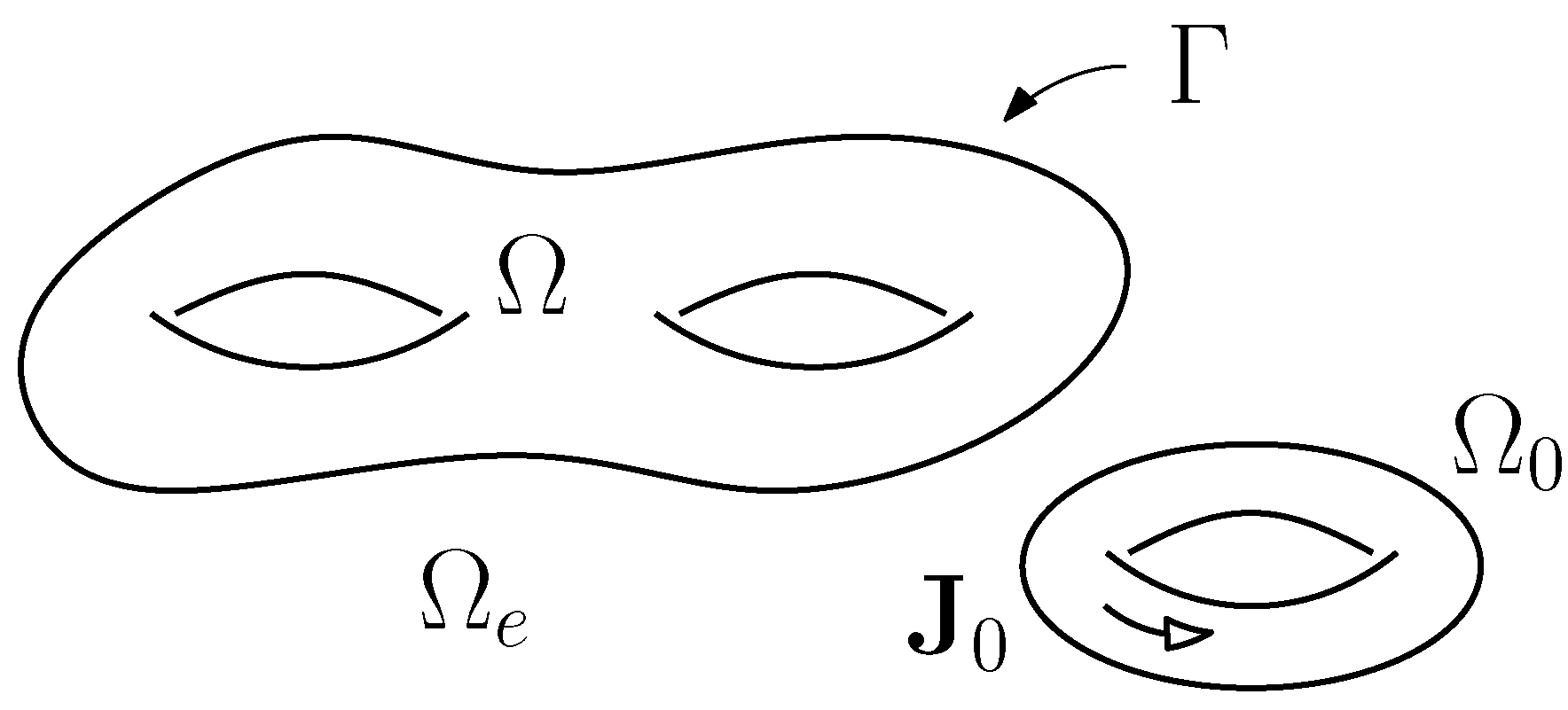
The computational domain of the eddy-current model is depicted in Figure 1. The interior region $\Omega ={\bigcup }_{k=1}^n{\Omega }_k$ is defined as the union of n open bounded and possibly multiply-connected subdomains ${\Omega }_k\subseteq {\mathbb{R}}^3$, $k=1\dots n$, which include conductive and/or magnetic linear materials. Let $\overline{\Omega }$ be the set closure of $\Omega$. The domain ${\Omega }_e={\mathbb{R}}^3\backslash \overline{\Omega }$ is then defined as the exterior region, which is unbounded and possibly multiply-connected, and includes field sources in the subdomain ${\Omega }_0\subseteq {\Omega }_e$. The air region can be possibly split between $\Omega$ and ${\Omega }_e$. Note also that ${\Omega }_0$ is strictly embedded in the exterior region, so that $\partial {\Omega }_0\cap \partial {\Omega }_e=\varnothing$. The interface between interior and exterior regions is the surface $\Gamma =\overline{\Omega }\cap {\overline{\Omega }}_e$, which can be partitioned into several connected components ${\Gamma }_k=\partial {\Omega }_k$, $k=1,\dots ,n$. Finally, it has to be noted that the surface $\Gamma$ is also the boundary of $\Omega$.

2.1. Interior Problem

In order to reduce the number of field problem variables, a magnetic vector potential $\mathbf{A}$, such that $\mathbf{E}=-ı\omega \mathbf{A}$, can be used [15]. By letting the vector potential in (2), it results in:

$$\mathbf{B}=\nabla \times \mathbf{A},$$

(9)

which implicitly fulfills (6) in $\Omega$. By eliminating the magnetic field variable from Ampère’s law (3) and by taking ${\mathbf{J}}_{\mathbf{0}}=\mathbf{0}$ since no source currents flow in the interior domain, the magnetic vector potential diffusion equation in $\Omega$ is obtained:

$$\nabla \times \nu \nabla \times \mathbf{A}+ı\omega \sigma \mathbf{A}=\mathbf{0}.$$

(10)

Note that the use of an “electric variable” $\mathbf{A}$ makes it possible to also model parts of $\Omega$ that are non-conducting (i.e., ${\Omega }_{nc}\subseteq \Omega$, with $\sigma =0$ locally), which is very common in practical engineering problems. On the other hand, for numerical computing purposes, the interior region has to be restricted as much as possible in order to reduce the mesh region and, in turn, the number of unknowns in the discretized model. (10) can be solved after imposing Dirichlet boundary conditions ${\gamma }_D\mathbf{A}$ on $\Gamma$, which are provided by interface conditions given in Section 2.2 and thus require the combined solution of the exterior field problem in Section 2.3. The solution of (10) is not unique if there exists any subdomain ${\Omega }_{nc}$, since $\mathbf{A}+\nabla u$ still fulfills (10) for any scalar potential u. Once $\mathbf{A}$ has been obtained, all other vector fields defined in $\Omega$ can be easily reconstructed.

2.2. Interface Conditions

The tangent component of the magnetic field $H_t$ and the normal component of the magnetic flux density $B_n$ need to be continuous across the interface $\Gamma$, which separates the interior region from the exterior region. In order to enforce the continuity of field components, suitable Dirichlet ${\gamma }_D$ and Neumann ${\gamma }_N$trace operators are defined [15]. For any smooth vector field $\mathbf{U}$ on $\Gamma$, there it holds:

$$\begin{array}{cc}\hfill {\gamma }_D\mathbf{U}& =\left(\mathbf{n}\times \mathbf{U}\right)\times \mathbf{n},\hfill \end{array}$$

(11)

$$\begin{array}{cc}\hfill {\gamma }_N\mathbf{U}& =\left(\nabla \times \mathbf{U}\right)\times \mathbf{n},\hfill \end{array}$$

(12)

where $\mathbf{n}$ is the exterior unit normal vector pointing from $\Omega$ to ${\Omega }_e$. Denoting with superscript + the exterior traces (i.e., approaching $\Gamma$ from outside along $\mathbf{n}$ direction) and with − the interior ones, the conservation of $B_n$ across $\Gamma$ can be recast as:

$${\gamma }_D^{-}\mathbf{A}={\gamma }_D^{+}\mathbf{A},$$

(13)

where ${\gamma }_D^{-}\mathbf{A}$ are the Dirichlet conditions for solving the interior problem. By noting that ${\Omega }_e$ does not include magnetic media (i.e., ${\nu }_0={\mu }_0^{-1}$, with ${\mu }_0$ air magnetic permeability), the conservation of $H_t$ across $\Gamma$ can be rephrased as:

$$\nu {\gamma }_N^{-}\mathbf{A}={\nu }_0{\gamma }_N^{+}\mathbf{A}.$$

(14)

2.3. Exterior Problem

The exterior region does not include any conductor by definition; therefore, eddy–currents are not present here. For ${\Omega }_e$, the following equations for magnetostatics hold:

$$\begin{array}{cc}\hfill \nabla \times \mathbf{H}& ={\mathbf{J}}_{\mathbf{0}},\hfill \end{array}$$

(15)

$$\begin{array}{cc}\hfill \mathbf{B}& ={\mu }_0\mathbf{H},\hfill \end{array}$$

(16)

complemented by Gauss’s law (6). The key idea of hybrid methods is to formulate the magnetostatic problem in the exterior region in integral form and to discretize it by means of the BEM, which does not require to use a volume mesh for discretizing Laplace’s equation and is suitable for analyzing unbounded field problems.

In hybrid formulations, the source magnetic field, generated by current density distribution ${\mathbf{J}}_0$, is analytically computed by using Biot–Savart’s law:

$${\mathbf{H}}_0\left(x\right)={\int }_{{\Omega }_0}\frac{{\mathbf{J}}_0\left(y\right)\times (x-y)}{{\parallel x-y\parallel }^3}dy,\mathrm{for}\mathrm{any}x\in {\mathbb{R}}^3\backslash {\overline{\Omega }}_0.$$

(17)

Therefore, the complementary part of the source field, i.e., ${\mathbf{H}}_c=\mathbf{H}-{\mathbf{H}}_0$, is curl-free due to (15). Any curl-free field is a representative of the first de Rham cohomology group $H_{dR}^1\left({\Omega }_e\right)=Z_{dR}^1\left({\Omega }_e\right)/B_{dR}^1\left({\Omega }_e\right)$ that is the quotient space of curl-free fields $Z_{dR}^1\left({\Omega }_e\right)$ and $B_{dR}^1\left({\Omega }_e\right)$ gradient fields [16]. The dimension of $H_{dR}^1\left({\Omega }_e\right)$ is proven to be equal to the first Betti number ${\beta }_1(\Omega )$ of the interior region $\Omega$. In other words, there exists an isomorphism between the cohomology of ${\Omega }_e$ and the homology $H_1(\Omega )$ of $\Omega$ [14]. This basic observation is key in order to derive the magnetic field decomposition in ${\Omega }_e$.

Since ${\mathbf{H}}_c\in Z_{dR}^1\left({\Omega }_e\right)$, in the most general case of a multiply-connected domain, i.e., ${\beta }_1(\Omega )\ge 1$, the complementary field in ${\Omega }_e$ can be represented as:

$${\mathbf{H}}_c=\nabla \phi +\sum _{k=1}^{{\beta }_1(\Omega )}{\alpha }_k{\mathbf{h}}_k,$$

(18)

where $\phi$ is a scalar potential, ${\alpha }_k$ are complex coefficients, and ${\mathbf{h}}_k$, $k=1,\dots ,{\beta }_1(\Omega )$, is the so-called cohomology basis, i.e., a vector basis of representatives of $H_{dR}^1\left({\Omega }_e\right)$. For simply connected domains, as $Z_{dR}^1\left({\Omega }_e\right)=B_{dR}^1\left({\Omega }_e\right)$, it turns out that any complementary field can be represented as a gradient. A possible choice for the cohomology basis is obtained by taking magnetic fields generated by filamentary loops ${\gamma }_k\subseteq \Omega$, $k=1,\dots ,{\beta }_1(\Omega )$, i.e., a set of generators of $H_1(\Omega )$, termed virtual fields, each one carrying a unit current [16]:

$${\mathbf{h}}_k\left(x\right)={\int }_{{\gamma }_k}\frac{{\mathbf{t}}_k\left(y\right)\times (x-y)}{{\parallel x-y\parallel }^3}d{\gamma }_y,\mathrm{for}\mathrm{any}x\in {\Omega }_e,$$

(19)

where ${\mathbf{t}}_k$ is the unit vector tangent to ${\gamma }_k$. Due to Poincaré duality, any virtual loop ${\gamma }_k$, i.e., a generator of $H_1(\Omega )$, is in one-to-one correspondence with a cutting surface ${\Sigma }_k$, i.e., a generator of $H_2(\Omega ,\partial \Omega )$. Through each cut, an independent virtual current $I_k={\int }_{{\Sigma }_k}\mathbf{J}·{\mathbf{n}}_{k}d\Sigma$, with ${\mathbf{n}}_k$ unit vector normal to ${\Sigma }_k$, can be defined as proven in [17]. By enforcing Ampère’s law around the boundary $\partial {\Sigma }_k$ of any cut, and by using (19) as generators, coefficients in (18) are proven to have physical meaning. These correspond to genuine eddy–currents flowing in the conductive region through cuts, as:

$$I_k={\int }_{\partial {\Sigma }_k}\mathbf{H}·\mathbf{t}d\gamma ={\int }_{\partial {\Sigma }_k}\left({\mathbf{H}}_0+\nabla \phi +\sum _{j=1}^{{\beta }_1(\Omega )}{\alpha }_j{\mathbf{h}}_j\right)·{\mathbf{t}}_{k}d\gamma ={\alpha }_k,$$

(20)

where ${\int }_{\partial {\Sigma }_k}{\mathbf{H}}_0·\mathbf{t}d\gamma =0$, for the source field, and ${\int }_{\partial {\Sigma }_k}{\mathbf{h}}_j·\mathbf{t}d\gamma ={\delta }_{kj}$, with ${\delta }_{kj}$ Kronecker delta, for any virtual field. In particular, the last integral is zero if boundary $\partial {\Sigma }_k$ does not link ${\gamma }_j$. By defining the reduced magnetic field as ${\mathbf{H}}_r=-\nabla {\phi }_r$, with ${\phi }_r$ reduced magnetic scalar potential, and by using (18) and (20), the magnetic field in ${\Omega }_e$ finally becomes:

$$\mathbf{H}={\mathbf{H}}_0+{\mathbf{H}}_r+\sum _{k=1}^{{\beta }_1(\Omega )}{I}_k{\mathbf{h}}_k.$$

(21)

For magnetostatic problems, for which $I_k=0$, or for quasi-magnetostatics problems with a simply-connected interior region, such that ${\beta }_1(\Omega )=0$, (21) reduces to the more simple form $\mathbf{H}={\mathbf{H}}_0-\nabla {\phi }_r$, and the scalar potential is uniquely defined in ${\Omega }_e$.

From (21), by imposing (6) and by noting that both ${\mathbf{H}}_0$ and any ${\mathbf{h}}_k$ are div-free, the so-called Exterior Neumann Problem (ENP) is obtained, i.e., to find a potential ${\phi }_r$ such that

$$\begin{array}{cccc}\hfill \nabla ·\left(-{\mu }_0\nabla {\phi }_r\right)& =0,\hfill & \hfill & \mathrm{in}{\Omega }_e\hfill \end{array}$$

(22)

$$\begin{array}{cccc}\hfill -{\mu }_0\nabla {\phi }_r·\mathbf{n}& =B_{r,n},\hfill & \hfill & \mathrm{on}\Gamma \hfill \end{array}$$

(23)

where $B_{r,n}$ is the normal component of the reduced magnetic flux density (i.e., the Neumann datum). These equations have to be supplemented by the decay condition obtained from (8), which states that the solution has to be harmonic at infinite:

$${\phi }_r\left(x\right)=\mathcal{O}\left({\parallel x\parallel }^{-1}\right),\mathrm{constantly}\mathrm{for}\parallel x\parallel \to \infty .$$

(24)

Potential ${\phi }_r$ is proven to be unique if the compatibility condition on the Neumann datum is fulfilled, i.e., ${\int }_{{\Gamma }_k}{B}_{r,n}d\Gamma =0$ for any connected component ${\Gamma }_k$, $k=1,\dots ,n$ [18]. This condition is naturally ensured by (22), which, for any connected component ${\Omega }_k$, provides:

$${\int }_{{\Gamma }_k}{B}_{r,n}d\Gamma ={\int }_{{\Omega }_k}\nabla ·{\mathbf{B}}_{r}d\Omega =0.$$

(25)

It is well known from the BEM literature that ${\phi }_r$ can be sought as a solution of an integral equation. There are typically two different (and equivalent) approaches for posing the ENP in integral form [19]: the direct formulation makes use of the second Green’s identity to obtain an integral equation formulated directly in terms of ${\phi }_r$, whereas the indirect formulation makes use of Fredholm’s theory to obtain an integral equation formulated in terms of an auxiliary variable (termed moment) to finally get ${\phi }_r$.

2.4. Direct Approach

The fundamental solution for the 3D Laplacian $\Phi (x,y)={\left(4\pi |x-y|\right)}^{-1}$ provides the scalar potential at any point x of the exterior domain ${\Omega }_e$, which is produced by a unit positive charge located at point $y\in {\Omega }_e$. Therefore, for any fixed y, it fulfills ${\Delta }_x\Phi (x,y)=-\delta (x-y)$, where the Laplacian acts only on the x variable and the Dirac delta $\delta$ represents the point source. In particular, the so-called sifting property holds:

$${\int }_{{\Omega }_e}{\phi }_r\left(x\right)\delta (x-y)dx=c\left(y\right){\phi }_r\left(y\right),$$

(26)

where $c\left(y\right)=\alpha \left(y\right)/\left(4\pi \right)$ is a geometric coefficient, in which $\alpha \left(y\right)$ is the solid angle subtended within ${\Omega }_e$ at point y. For instance, $c\left(y\right)=1/2$ for a point lying on a smooth part of the boundary $\partial {\Omega }_e$, i.e., with tangent plane, and $c\left(y\right)=1$ for a point inside ${\Omega }_e$.

By testing $\Delta {\phi }_r=0$ with the fundamental solution and by using (26), the Green’s second identity is obtained for almost any $y\in {\Omega }_e$ [20,21]:

$$c\left(y\right){\phi }_r\left(y\right)+{\int }_{\partial {\Omega }_e}{\phi }_r\left(x\right)\frac{\partial \Phi (x,y)}{\partial n_x^{\prime }}d{\sigma }_x={\int }_{\partial {\Omega }_e}\Phi (x,y)\frac{\partial {\phi }_r\left(x\right)}{\partial n_x^{\prime }}d{\sigma }_x.$$

(27)

The exterior normal derivative is the directional derivative carried out with respect to the x variable along the outward unit normal ${\mathbf{n}}^{\prime }\left(x\right)$ of ${\Omega }_e$ and approaching the boundary $\partial {\Omega }_e$ from the outside. For any smooth function u, this can be rephrased as [18]:

$$\frac{\partial u\left(x\right)}{\partial n_x^{\prime }}=\underset{t\to 0^{+}}{lim}{\mathbf{n}}^{\prime }\left(x\right)·\nabla u(x+t{\mathbf{n}}^{\prime }\left(x\right)).$$

(28)

In (27), only the “finite” part of boundary integral, i.e., that one over $\Gamma$, has to be considered due to decay condition (24). It has to be noted, however, that the orientation of $\Gamma$, which is the boundary of $\Omega$, is opposite to that one of $\partial {\Omega }_e$, i.e., ${\mathbf{n}}^{\prime }=-\mathbf{n}$, so that:

$$\frac{\partial {\phi }_r\left(x\right)}{\partial n_x^{\prime }}=-\frac{\partial {\phi }_r\left(x\right)}{\partial n_x}={\nu }_0{B}_{r,n}\left(x\right),\mathrm{for}\mathrm{any}x\in \Gamma .$$

(29)

By letting (29) in (27), the direct boundary integral equation is obtained:

$$c\left(y\right){\phi }_r\left(y\right)+{\int }_{\Gamma }{\phi }_r\left(x\right)\frac{\partial \Phi (x,y)}{\partial n_x^{\prime }}d{\sigma }_x={\nu }_0{\int }_{\Gamma }\Phi (x,y)B_{r,n}\left(x\right)d{\sigma }_x,\mathrm{for}\mathrm{a}.\mathrm{a}.y\in {\Omega }_e.$$

(30)

Note that, when y lies on the surface $\Gamma$, integrals in (30) have to be intended in a principal value sense, i.e., obtained as a limit by taking an infinitesimal neighborhood around the singularity y.

The boundary integral Equation (30) is equivalent to the ENP and states a direct relationship between the Dirichlet datum, i.e., the scalar potential on $\Gamma$, and the Neumann datum. Once boundary quantities have been computed, the scalar potential can be reconstructed in the air region by using (30) with $c\left(y\right)=1$. It has to be observed, however, that the computation of the magnetic field by (21) requires the numerical differentiation of ${\phi }_r$, which typically involves a multiple field sampling around any fixed y. On the other hand, an analytical differentiation of (30) leads to hyper-singular integrals, which cannot be accurately computed for points close to $\Gamma$ as discussed in [22].

2.5. Indirect Approach

The ENP can be solved also by means of the so-called method of layer potentials used in potential theory [18]. ${\phi }_r$ in ${\Omega }_e$ can be generated by an equivalent single-layer magnetic charge density distribution q over $\Gamma$, across which the field normal component $B_{r,n}$ jumps. The single-layer integral operator with moment q is defined as [23]:

$${\phi }_r\left(x\right)=K\left[q\right]\left(x\right)={\int }_{\Gamma }\Phi (x,y)q\left(y\right)d{\sigma }_y.$$

(31)

If Neumann datum fulfills the compatibility condition (25), the equivalent source q is proven to be the unique solution of the following Fredholm integral equation [18,24]:

$${\mu }_{0}c\left(x\right)+{\mathcal{T}}^{*}\left[q\right]\left(x\right)=B_{r,n}\left(x\right),\mathrm{for}\mathrm{a}.\mathrm{a}.x\in \Gamma ,$$

(32)

The adjoint double-layer integral operator in (32) is defined as:

$${\mathcal{T}}^{*}\left[q\right]\left(x\right)=-{\mu }_0{\int }_{\Gamma }q\left(y\right)\frac{\partial \Phi (x,y)}{\partial n_x}d{\sigma }_y,$$

(33)

where the normal derivative is evaluated along the unit normal vector $\mathbf{n}$ defined above. Differently from (30), the Fredholm equation does not establish a direct correspondence between the potential and its normal derivative on $\Gamma$. ${\phi }_r$ can be reconstructed with (31) once the equivalent charge distribution has been found from (32), for a given $B_{r,n}$. By eliminating the auxiliary variable, one obtains the so-called Steklov–Poincaré operator or Dirichlet-to-Neumann (DN) map, which maps the Dirichlet to the Neumann datum:

$$B_{r,n}\left(x\right)=S\left[{\phi }_r\right]\left(x\right)={\mu }_{0}c\left(x\right)+{\mathcal{T}}^{*}\circ K^{-1}\left[{\phi }_r\right]\left(x\right),\mathrm{for}\mathrm{a}.\mathrm{a}.x\in \Gamma .$$

(34)

It has to be noted that the indirect formulation allows for an easier post-processing since the magnetic field can be obtained from the equivalent magnetic charge distribution. For any field point x in ${\Omega }_e$, which is an open set by definition, (31) results in being infinitely differentiable. Therefore, by taking the gradient of (31), the reduced field becomes:

$${\mathbf{H}}_r\left(x\right)=-{\int }_{\Gamma }\nabla {}_x\Phi (x,y)q\left(y\right)d{\sigma }_y,\mathrm{for}\mathrm{any}x\in {\Omega }_e.$$

(35)

Finally, the magnetic flux density distribution in the exterior domain can be obtained by inserting (35) in (21) and by using the magnetic constitutive relationship (16).

3. Cell Method with Augmented Dual Grid

In this work, the interior problem is discretized with the CM, instead of the much more common FEM. The key steps of such a discretization process are examined in detail, starting from the CM variant based on augmented dual grids presented in [11]. A similar construction, for tetrahedral meshes, is also reported in [25] for a pure–CM formulation, which is suitable for solving eddy–current problems in bounded domains. Note that this is completely general, and can be extended to polyhedral meshes [26].

Any connected component ${\Omega }_i\subseteq \Omega$ is discretized by its domain primal grid ${\mathcal{G}}_{{\Omega }_i}$, with $N_{{\Omega }_i}$ nodes, $E_{{\Omega }_i}$ edges, $F_{{\Omega }_i}$ faces, and $V_{{\Omega }_i}$ cells. The boundary primal grid ${\mathcal{G}}_{\partial {\Omega }_i}$ is the restriction of ${\mathcal{G}}_{{\Omega }_i}$ to its boundary $\partial {\Omega }_i$, where nodes are traces of bulk primal edges of ${\mathcal{G}}_{{\Omega }_i}$, edges are traces of bulk primal faces, and faces are traces of bulk primal cells. ${\mathcal{G}}_{{\Omega }_i}$ and ${\mathcal{G}}_{\partial {\Omega }_i}$ are then partitioned into their corresponding barycentric subdivisions, which are obtained by splitting any cell or boundary cell into a set of tetrahedrons or triangles having as a common apex the cell center. The domain dual grid ${\tilde{\mathcal{G}}}_{{\Omega }_i}$, with ${\tilde{N}}_{{\Omega }_i}$ nodes, ${\tilde{E}}_{{\Omega }_i}$ edges, ${\tilde{F}}_{{\Omega }_i}$ faces, and ${\tilde{V}}_{{\Omega }_i}$ cells, and the boundary dual grid ${\tilde{\mathcal{G}}}_{\partial {\Omega }_i}$ are built by aggregating barycentric cells of ${\mathcal{G}}_{{\Omega }_i}$ and ${\mathcal{G}}_{\partial {\Omega }_i}$, respectively, around primal nodes. This specific geometric construction provides a one-to-one correspondence between primal and dual grid entities so that ${\tilde{N}}_{{\Omega }_i}=V_{{\Omega }_i}$, ${\tilde{E}}_{{\Omega }_i}=F_{{\Omega }_i}$, ${\tilde{F}}_{{\Omega }_i}=E_{{\Omega }_i}$, and ${\tilde{V}}_{{\Omega }_i}=N_{{\Omega }_i}$. Similar relationships hold for ${\mathcal{G}}_{\partial {\Omega }_i}$. Finally, the augmented dual grid is defined as the union of dual grids, i.e., ${\tilde{\mathcal{G}}}_{{\Omega }_i\partial {\Omega }_i}={\tilde{\mathcal{G}}}_{{\Omega }_i}\cup {\tilde{\mathcal{G}}}_{\partial {\Omega }_i}$. Primal and dual grids of the interface $\Gamma$, represented in Figure 1, are inherited from those on $\partial \Omega$ such that ${\mathcal{G}}_{\Gamma }={\mathcal{G}}_{\partial \Omega }$ and ${\tilde{\mathcal{G}}}_{\Gamma }={\tilde{\mathcal{G}}}_{\partial \Omega }$.

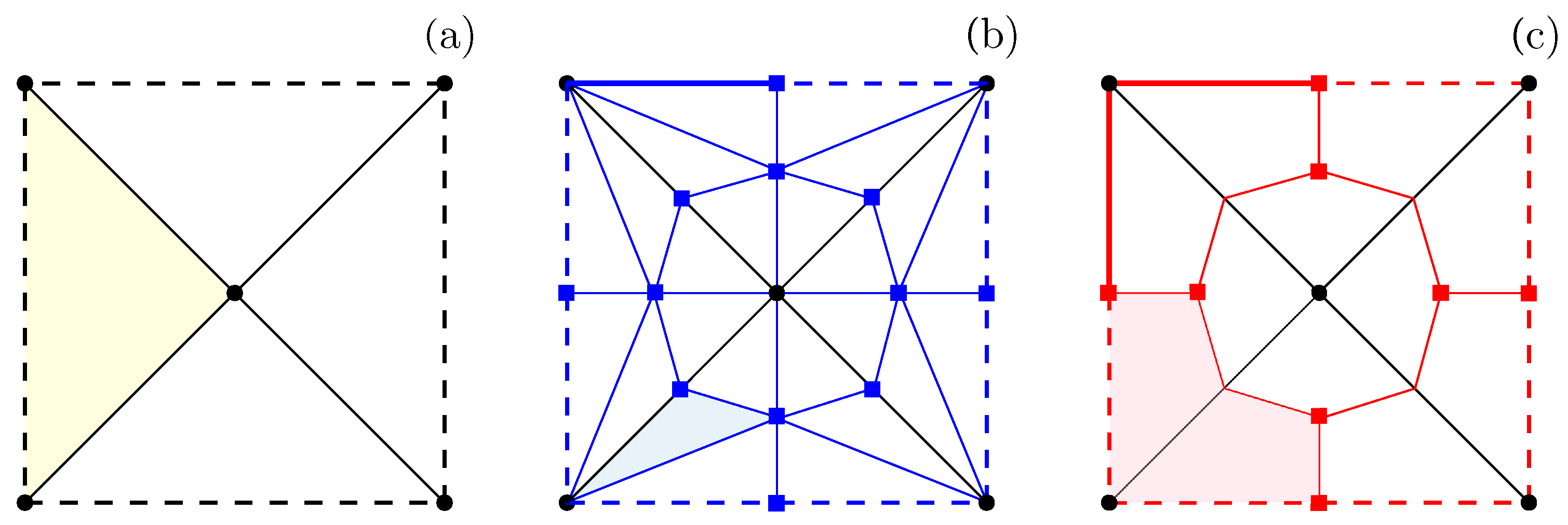
To illustrate such a geometric construction, the 2D example provided in [25] is discussed here in detail. A unit square $\Omega ={[0,1]}^2$ is meshed into a primal grid ${\mathcal{G}}_{\Omega }$ made of triangles (Figure 2a). The augmented dual grid ${\tilde{\mathcal{G}}}_{\Omega \partial \Omega }$ in Figure 2c is obtained by assembling triangles of the barycentric subdivision ${\mathcal{G}}_{\Omega }^{\Delta }$ (Figure 2b). Any dual cell (polygon in light red) is obtained by aggregating barycentric triangles (in light blue) around any primal node (black dots). In such a way, a one-to-one correspondence between primal nodes and dual cells is obtained. Dual nodes (red dots) are centers of domain and boundary primal cells. In the same way, on the domain boundary, ${\tilde{\mathcal{G}}}_{\partial \Omega }$, made up of 1D dual cells, is constructed by aggregating 1D barycentric cells. The other way round, a one-to-one correspondence exists also between dual nodes and primal cells, which can be either primal cells of ${\mathcal{G}}_{\Omega }$ or boundary edges of ${\mathcal{G}}_{\partial \Omega }$.

3.1. Discrete Field Variables

According to the original CM discretization scheme proposed by Tonti [4], problem variables (DOFs) can be either scalar potentials evaluated at nodes or integrals over edges, faces, or cells of the meshed domain. DOFs are defined upon orientation of the corresponding geometric entity. In fact, similarly to physical quantities of electric circuits, sign convention is related to the orientation of the geometric entity.

Geometric entities of the primal grid ${\mathcal{G}}_{\Omega }$ are inner oriented, which means that nodes are oriented as sinks, edges are directed from one end to the other, faces are oriented by crossing their boundary clockwise or counterclockwise, and cells are oriented by assuming that their faces are all oriented in the same way. Boundary geometric entities are a subset of those in ${\mathcal{G}}_{\Omega }$. Geometric entities of the augmented dual grid ${\tilde{\mathcal{G}}}_{\Omega \partial \Omega }$ are outer oriented, which simply amounts to inheriting the orientation from ${\mathcal{G}}_{\Omega }$ and ${\mathcal{G}}_{\Gamma }$. In fact, any dual entity is one-to-one correspondence with a primal entity, endowed by an inner orientation. For instance, any dual edge is oriented by a clockwise or counterclockwise rotation around it, i.e., the inner orientation of its corresponding primal face.

For the eddy–current model in $\Omega$, discrete field variables are: the electromotive forces (emfs) along primal edges e, i.e., ${\mathbf{e}}_{\Omega }={\left(e_e\right)}_{e\in {\mathcal{G}}_{\Omega }}$, where $e_e={\int }_e\mathbf{E}·\mathbf{t}d\gamma$ and $\mathbf{t}$ is the unit tangent vector related to e; magnetic vector potential line integrals ${\mathbf{a}}_{\Omega }={\left(a_e\right)}_{e\in {\mathcal{G}}_{\Omega }}$, with $a_e={\int }_e\mathbf{A}·\mathbf{t}d\gamma$; magnetic fluxes through primal faces f, i.e., ${\mathbf{b}}_{\Omega }={\left(b_f\right)}_{f\in {\mathcal{G}}_{\Omega }}$, where $b_f={\int }_f\mathbf{B}·\mathbf{n}d\sigma$ and $\mathbf{n}$ is the unit normal vector related to f; magnetomotive forces (mmfs) along dual edges $\tilde{e}$, i.e., ${\tilde{\mathbf{h}}}_{\Omega }={\left({\tilde{h}}_{\tilde{e}}\right)}_{\tilde{e}\in {\tilde{\mathcal{G}}}_{\Omega \Gamma }}$, with ${\tilde{h}}_{\tilde{e}}={\int }_{\tilde{e}}\mathbf{H}·\mathbf{t}d\gamma$; electric currents through dual faces $\tilde{f}$, i.e., ${\tilde{\mathbf{j}}}_{\Omega }={\left({\tilde{j}}_{\tilde{f}}\right)}_{\tilde{f}\in {\tilde{\mathcal{G}}}_{\Omega \Gamma }}$, with ${\tilde{j}}_{\tilde{f}}={\int }_{\tilde{f}}\mathbf{J}·\mathbf{n}d\sigma$. Similar arrays of DOFs are defined on primal and dual grids of $\Gamma$, e.g., reduced magnetic potentials on interface dual nodes ${\tilde{\mathit{\phi }}}_{\Gamma }$ and mmfs on interface dual edges ${\tilde{\mathbf{h}}}_{\Gamma }$.

3.2. Topological Operators

Local reference frames are related together by the connectivity between elements. An incidence number is $+1$ if a pair of connected geometric entities carries the same orientation, $-1$ otherwise, and 0 if they are disconnected. Incidence matrices with integer coefficients, which are the discrete counterparts of gradient, divergence, curl differential operators, can be defined on both primal and augmented dual grids [11].

For any bounded subdomain ${\Omega }_i$, the topological description of the primal grid ${\mathcal{G}}_{{\Omega }_i}$ is provided by the $E_{{\Omega }_i}\times N_{{\Omega }_i}$ edge–node incidence matrix ${\mathbf{G}}_{{\Omega }_i}$, the $F_{{\Omega }_i}\times E_{{\Omega }_i}$ face–edge incidence matrix ${\mathbf{C}}_{{\Omega }_i}$, and the $V_{{\Omega }_i}\times F_{{\Omega }_i}$ cell–face incidence matrix ${\mathbf{D}}_{{\Omega }_i}$. In addition, as it is well known from combinatorial topology, the following orthogonality properties hold [2]:

$$\begin{array}{cc}\hfill & {\mathbf{D}}_{{\Omega }_i}{\mathbf{C}}_{{\Omega }_i}=\mathbf{0},\hfill \end{array}$$

(36)

$$\begin{array}{cc}\hfill & {\mathbf{C}}_{{\Omega }_i}{\mathbf{G}}_{{\Omega }_i}=\mathbf{0}.\hfill \end{array}$$

(37)

These properties are required in order to obtain a cochain complex for ${\mathcal{G}}_{{\Omega }_i}$, mimicking the de Rham cohomology (with grad, div, curl operators) at the continuous level [2].

Similarly, the topological description of ${\tilde{\mathcal{G}}}_{{\Omega }_i}$ is provided by the $F_{{\Omega }_i}\times V_{{\Omega }_i}$ edge–node incidence matrix ${\tilde{\mathbf{G}}}_{{\Omega }_i}=-{\mathbf{D}}_{{\Omega }_i}^{\mathrm{T}}$, the $E_{{\Omega }_i}\times F_{{\Omega }_i}$ face–edge incidence matrix ${\tilde{\mathbf{C}}}_{{\Omega }_i}={\mathbf{C}}_{{\Omega }_i}^{\mathrm{T}}$, and the $N_{{\Omega }_i}\times E_{{\Omega }_i}$ cell–face incidence matrix ${\tilde{\mathbf{D}}}_{{\Omega }_i}=-{\mathbf{G}}_{{\Omega }_i}^{\mathrm{T}}$. From (36) and (37), the following orthogonality properties also hold:

$$\begin{array}{cc}\hfill & {\tilde{\mathbf{D}}}_{{\Omega }_i}{\tilde{\mathbf{C}}}_{{\Omega }_i}=\mathbf{0},\hfill \end{array}$$

(38)

$$\begin{array}{cc}\hfill & {\tilde{\mathbf{C}}}_{{\Omega }_i}{\tilde{\mathbf{G}}}_{{\Omega }_i}=\mathbf{0}.\hfill \end{array}$$

(39)

The augmented dual grid contains additional geometric entities, compared to ${\tilde{\mathcal{G}}}_{{\Omega }_i}$, that are dual nodes, edges, and faces on $\partial {\Omega }_i$. This leads to new incidence matrices relating dual entities of ${\tilde{\mathcal{G}}}_{{\Omega }_i}$ to those of ${\tilde{G}}_{\partial {\Omega }_i}$, that is: ${\tilde{\mathbf{G}}}_{{\Omega }_i\cap \partial {\Omega }_i}$ is the $F_{{\Omega }_i}\times F_{\partial {\Omega }_i}$ edge–node incidence matrix, ${\tilde{\mathbf{C}}}_{{\Omega }_i\cap \partial {\Omega }_i}$ is the $E_{{\Omega }_i}\times E_{\partial {\Omega }_i}$ face–edge incidence matrix, and ${\tilde{\mathbf{D}}}_{{\Omega }_i\cap \partial {\Omega }_i}$ is the $N_{{\Omega }_i}\times N_{\partial {\Omega }_i}$ cell–face incidence matrix. Any column of these matrices has a unique non-zero coefficient ($\pm 1$), which identifies the elements of ${\mathcal{G}}_{{\Omega }_i}$ that are in ${\mathcal{G}}_{\partial {\Omega }_i}$. Note that the transposed matrix of each of these incidence matrices is a selection matrix, which extracts DOFs related to the boundary primal grid from those of ${\mathcal{G}}_{\Omega }$.

The cell–face ${\tilde{\mathbf{D}}}_{{\Omega }_i\partial {\Omega }_i}$, the face–edge ${\tilde{\mathbf{C}}}_{{\Omega }_i\partial {\Omega }_i}$, and the edge–node ${\tilde{\mathbf{G}}}_{{\Omega }_i\partial {\Omega }_i}$ incidence matrices of ${\tilde{\mathcal{G}}}_{{\Omega }_i\partial {\Omega }_i}$ can be derived from the previous incidence matrices as [11]:

$$\begin{array}{cc}\hfill & {\tilde{\mathbf{D}}}_{{\Omega }_i\partial {\Omega }_i}=\left[\begin{array}{cc}{\tilde{\mathbf{D}}}_{{\Omega }_i}& {\tilde{\mathbf{D}}}_{{\Omega }_i\cap \partial {\Omega }_i}\end{array}\right],\hfill \end{array}$$

(40)

$$\begin{array}{cc}\hfill & {\tilde{\mathbf{C}}}_{{\Omega }_i\partial {\Omega }_i}=\left[\begin{array}{cc}{\tilde{\mathbf{C}}}_{{\Omega }_i}& {\tilde{\mathbf{C}}}_{{\Omega }_i\cap \partial {\Omega }_i}\\ \mathbf{0}& -{\tilde{\mathbf{D}}}_{{\Omega }_i\cap \partial {\Omega }_i}^{\mathrm{T}}{\tilde{\mathbf{D}}}_{{\Omega }_i}{\tilde{\mathbf{C}}}_{{\Omega }_i\cap \partial {\Omega }_i}\end{array}\right],\hfill \end{array}$$

(41)

$$\begin{array}{cc}\hfill & {\tilde{\mathbf{G}}}_{{\Omega }_i\partial {\Omega }_i}=\left[\begin{array}{cc}{\tilde{\mathbf{G}}}_{{\Omega }_i}& {\tilde{\mathbf{G}}}_{{\Omega }_i\cap \partial {\Omega }_i}\\ \mathbf{0}& -{\tilde{\mathbf{C}}}_{{\Omega }_i\cap \partial {\Omega }_i}^{\mathrm{T}}{\tilde{\mathbf{C}}}_{{\Omega }_i}{\tilde{\mathbf{G}}}_{{\Omega }_i\cap \partial {\Omega }_i}\end{array}\right].\hfill \end{array}$$

(42)

It can be proven that a cochain complex can be constructed also for the augmented dual grid. By observing that any face of ${\tilde{\mathcal{G}}}_{\partial {\Omega }_i}$ belongs only to one cell of ${\tilde{\mathcal{G}}}_{{\Omega }_i}$, one obtains:

$${\tilde{\mathbf{D}}}_{{\Omega }_i}{\tilde{\mathbf{C}}}_{{\Omega }_i\cap \partial {\Omega }_i}={\tilde{\mathbf{D}}}_{{\Omega }_i\cap \partial {\Omega }_i}{\tilde{\mathbf{D}}}_{{\Omega }_i\cap \partial {\Omega }_i}^{\mathrm{T}}{\tilde{\mathbf{D}}}_{{\Omega }_i}{\tilde{\mathbf{C}}}_{{\Omega }_i\cap \partial {\Omega }_i},$$

(43)

which provides:

$$\begin{array}{cc}\hfill {\tilde{\mathbf{D}}}_{{\Omega }_i\partial {\Omega }_i}{\tilde{\mathbf{C}}}_{{\Omega }_i\partial {\Omega }_i}& =\left[\begin{array}{cc}{\tilde{\mathbf{D}}}_{{\Omega }_i}& {\tilde{\mathbf{D}}}_{\partial {\Omega }_i}\end{array}\right]\left[\begin{array}{cc}{\tilde{\mathbf{C}}}_{{\Omega }_i}& {\tilde{\mathbf{C}}}_{{\Omega }_i\cap \partial {\Omega }_i}\\ \mathbf{0}& -{\tilde{\mathbf{D}}}_{{\Omega }_i\cap \partial {\Omega }_i}^{\mathrm{T}}{\tilde{\mathbf{D}}}_{{\Omega }_i}{\tilde{\mathbf{C}}}_{{\Omega }_i\cap \partial {\Omega }_i}\end{array}\right]\hfill \\ & =\left[\begin{array}{cc}{\tilde{\mathbf{D}}}_{{\Omega }_i}{\tilde{\mathbf{C}}}_{{\Omega }_i}& {\tilde{\mathbf{D}}}_{{\Omega }_i}{\tilde{\mathbf{C}}}_{{\Omega }_i\cap \partial {\Omega }_i}-{\tilde{\mathbf{D}}}_{{\Omega }_i\cap \partial {\Omega }_i}{\tilde{\mathbf{D}}}_{{\Omega }_i\cap \partial {\Omega }_i}^{\mathrm{T}}{\tilde{\mathbf{D}}}_{{\Omega }_i}{\tilde{\mathbf{C}}}_{{\Omega }_i\cap \partial {\Omega }_i}\end{array}\right]=\mathbf{0}.\hfill \end{array}$$

(44)

Similarly, noting that any edge of ${\tilde{\mathcal{G}}}_{\partial {\Omega }_i}$ belong only to one face of ${\tilde{\mathcal{G}}}_{{\Omega }_i}$, it ensues:

$${\tilde{\mathbf{C}}}_{{\Omega }_i}{\tilde{\mathbf{G}}}_{{\Omega }_i\cap \partial {\Omega }_i}={\tilde{\mathbf{C}}}_{{\Omega }_i\cap \partial {\Omega }_i}{\tilde{\mathbf{C}}}_{{\Omega }_i\cap \partial {\Omega }_i}^{\mathrm{T}}{\tilde{\mathbf{C}}}_{{\Omega }_i}{\tilde{\mathbf{G}}}_{{\Omega }_i\cap \partial {\Omega }_i},$$

(45)

which provides:

$$\begin{array}{cc}\hfill {\tilde{\mathbf{C}}}_{{\Omega }_i\partial {\Omega }_i}{\tilde{\mathbf{G}}}_{{\Omega }_i\partial {\Omega }_i}& =\left[\begin{array}{cc}{\tilde{\mathbf{C}}}_{{\Omega }_i}& {\tilde{\mathbf{C}}}_{{\Omega }_i\cap \partial {\Omega }_i}\\ \mathbf{0}& -{\tilde{\mathbf{D}}}_{{\Omega }_i\cap \partial {\Omega }_i}^{\mathrm{T}}\tilde{\mathbf{D}}{\tilde{\mathbf{C}}}_{{\Omega }_i\cap \partial {\Omega }_i}\end{array}\right]\left[\begin{array}{cc}{\tilde{\mathbf{G}}}_{{\Omega }_i}& {\tilde{\mathbf{G}}}_{{\Omega }_i\cap \partial {\Omega }_i}\\ \mathbf{0}& -{\tilde{\mathbf{C}}}_{{\Omega }_i\cap \partial {\Omega }_i}^{\mathrm{T}}\tilde{\mathbf{C}}{\tilde{\mathbf{G}}}_{{\Omega }_i\cap \partial {\Omega }_i}\end{array}\right]\hfill \\ & =\left[\begin{array}{cc}{\tilde{\mathbf{C}}}_{{\Omega }_i}{\tilde{\mathbf{G}}}_{{\Omega }_i}& {\tilde{\mathbf{C}}}_{{\Omega }_i}{\tilde{\mathbf{G}}}_{{\Omega }_i\cap \partial {\Omega }_i}-{\tilde{\mathbf{C}}}_{{\Omega }_i\cap \partial {\Omega }_i}{\tilde{\mathbf{C}}}_{{\Omega }_i\cap \partial {\Omega }_i}^{\mathrm{T}}{\tilde{\mathbf{C}}}_{{\Omega }_i}{\tilde{\mathbf{G}}}_{{\Omega }_i\cap \partial {\Omega }_i}\\ \mathbf{0}& {\tilde{\mathbf{D}}}_{{\Omega }_i\cap \partial {\Omega }_i}^{\mathrm{T}}{\tilde{\mathbf{D}}}_{{\Omega }_i}{\tilde{\mathbf{C}}}_{{\Omega }_i\cap \partial {\Omega }_i}{\tilde{\mathbf{C}}}_{{\Omega }_i\cap \partial {\Omega }_i}^{\mathrm{T}}{\tilde{\mathbf{C}}}_{{\Omega }_i}{\tilde{\mathbf{G}}}_{{\Omega }_i\cap \partial {\Omega }_i}\end{array}\right]=\mathbf{0}.\hfill \end{array}$$

(46)

Finally, in order to construct hybrid formulations, incidence matrices for the boundary mesh also need to introduced. For the primal boundary ${\mathcal{G}}_{\partial {\Omega }_i}$, the $E_{\partial {\Omega }_i}\times N_{\partial {\Omega }_i}$ edge–node incidence matrix ${\mathbf{G}}_{\partial {\Omega }_i}$ and the $F_{\partial {\Omega }_i}\times E_{\partial {\Omega }_i}$ face–edge incidence matrix ${\mathbf{C}}_{\partial {\Omega }_i}$. The corresponding dual operators can be defined from primal ones as follows: the edge–node incidence matrix is ${\tilde{\mathbf{G}}}_{\partial {\Omega }_i}={\mathbf{C}}_{\partial {\Omega }_i}^{\mathrm{T}}$ and the face–edge incidence matrix is ${\tilde{\mathbf{C}}}_{\partial {\Omega }_i}={\mathbf{G}}_{\partial {\Omega }_i}^{\mathrm{T}}$.

3.3. Discrete Constitutive Relations

A systematic approach for building edge and face vector basis functions for grids composed of either oblique parallelepipeds or oblique triangular prisms or tetrahedra is proposed in [5]. The same approach is extended in [7] to general polyhedral grids. The main results of the so-called energy approach presented in [5] are outlined here.

For the eddy–current model, linear conductive and magnetic media, with piecewise constant conductivity $\sigma$ and reluctivity $\nu$, are assumed in $\Omega$. Local constitutive relationships $\mathbf{J}=\sigma \mathbf{E}$ and $\mathbf{H}=\nu \mathbf{B}$ are discretized by expanding $\mathbf{E}$ and $\mathbf{B}$ in terms of DOFs with piecewise constant edge ${\mathbf{w}}_e$ and face ${\mathbf{w}}_f$ vector basis functions. It is noted that these basis functions are suitable for CM but not for FEM, since they exhibit less regularity than that required by the FEM. The energy approach starts from the assumption that, by using these vector functions, energy has to be exactly reconstructed inside any cell of ${\mathcal{G}}_{\Omega }$ for any locally constant field.

The electric field can be globally approximated by the following expansion:

$$\mathbf{E}\left(x\right)\approx \sum _{e=1}^{E_{\Omega }}{\mathbf{w}}_e\left(x\right)e_e,\mathrm{for}\mathrm{any}x\in \Omega ,$$

(47)

where $e_e$ is the emf along the eth edge of ${\mathcal{G}}_{\Omega }$, i.e., a DOF of the array ${\mathbf{e}}_{\Omega }$. The support of ${\mathbf{w}}_e$ is compact, and it consists of the union of all the non-empty intersections ${\omega }_e$ between any primal cell incident to e and any dual cell centered on any vertex of e. The edge function is locally constant inside these intersections, and it is defined as:

$${\mathbf{w}}_e\left(x\right)=\frac{{\mathbf{e}}_j\times {\mathbf{e}}_k}{{\mathbf{e}}_e\times {\mathbf{e}}_j·{\mathbf{e}}_k},\mathrm{for}\mathrm{any}x\in {\omega }_e,$$

(48)

where ${\mathbf{e}}_e$, ${\mathbf{e}}_j$, and ${\mathbf{e}}_k$ are the edge vectors of primal edges incident to ${\omega }_e$.

Since source current density is null in $\Omega$, local Ohm’s law (4) becomes $\mathbf{J}=\sigma \mathbf{E}$. From this relationship and (47), the overall electric power loss in $\Omega$ is obtained as:

$$\begin{array}{cc}\hfill P_{\Omega }=\frac{1}{2}{\int }_{\Omega }{\mathbf{E}}^{*}\left(x\right)·\sigma \left(x\right)\mathbf{E}\left(x\right)dx& =\frac{1}{2}{\int }_{\Omega }\sum _{e=1}^{E_{\Omega }}{\mathbf{w}}_e\left(x\right)e_e^{*}·\sigma \left(x\right)\sum _{e^{\prime }=1}^{E_{\Omega }}{\mathbf{w}}_{e^{\prime }}\left(x\right)e_{e^{\prime }}dx\hfill \\ & =\frac{1}{2}\sum _{e=1}^{E_{\Omega }}\sum _{e^{\prime }=1}^{E_{\Omega }}{e}_e^{*}\left({\int }_{\Omega }{\mathbf{w}}_{e^{\prime }}\left(x\right)·\sigma \left(x\right){\mathbf{w}}_e\left(x\right)dx\right)e_e\hfill \\ & =\frac{1}{2}{\mathbf{e}}_{\Omega }^{*}{\mathbf{M}}_{\sigma ,\Omega }{\mathbf{e}}_{\Omega },\hfill \end{array}$$

(49)

where * indicates the hermitian operator for complex-valued quantities. The conductance matrix ${\mathbf{M}}_{\sigma ,\Omega }={\left(m_{\sigma ,e{e}^{\prime }}\right)}_{e,e^{\prime }\in {\mathcal{G}}_{\Omega }}$ of size $E_{\Omega }\times E_{\Omega }$ is defined as:

$$m_{\sigma ,e{e}^{\prime }}={\int }_{\Omega }{\mathbf{w}}_e\left(x\right)·\sigma \left(x\right){\mathbf{w}}_{e^{\prime }}\left(x\right)dx.$$

(50)

As proven in [5], the conductance matrix is symmetric and positive definite. The so-called consistency property holds for edge vector basis vectors, namely:

$$\begin{array}{cc}\hfill & {\int }_{\Omega }{\mathbf{w}}_e\left(\mathbf{r}\right)dx={\tilde{\mathbf{f}}}_e,\hfill \end{array}$$

(51)

where ${\tilde{\mathbf{f}}}_e$ is the face vector of the dual face in one-to-one correspondence with e. This fundamental property ensures that ${\mathbf{M}}_{\sigma ,\Omega }{\mathbf{e}}_{\Omega }$ is an approximation of ${\tilde{\mathbf{j}}}_{\Omega }$. In particular, the electric constitutive relationship:

$${\tilde{\mathbf{j}}}_{\Omega }={\mathbf{M}}_{\sigma ,\Omega }{\mathbf{e}}_{\Omega },$$

(52)

is exactly fulfilled for any field $\mathbf{E}$ that is piecewise constant in primal cells.

Similarly to (47), the magnetic flux density is globally approximated as:

$$\mathbf{B}\left(x\right)\approx \sum _{f=1}^{F_{\Omega }}{\mathbf{w}}_f\left(x\right)b_f,\mathrm{for}\mathrm{any}x\in \Omega ,$$

(53)

where $b_f$ is the magnetic flux through the f-th face of ${\mathcal{G}}_{\Omega }$, i.e., a DOF of the array ${\mathbf{b}}_{\Omega }$. The support of ${\mathbf{w}}_f$ is compact, and it consists of the union of all the non-empty intersections ${\omega }_f$ between any primal cell incident to f and any dual cell centered on any vertex of f. The face function is locally constant inside these intersections, and it is defined as:

$${\mathbf{w}}_f\left(x\right)=\frac{{\mathbf{f}}_j\times {\mathbf{f}}_k}{{\mathbf{f}}_f\times {\mathbf{f}}_j·{\mathbf{f}}_k},\mathrm{for}\mathrm{any}x\in {\omega }_f,$$

(54)

where ${\mathbf{f}}_f$, ${\mathbf{f}}_j$, and ${\mathbf{f}}_k$ are the face vectors of primal faces incident to ${\omega }_f$.

From the local magnetic constitutive relationships (5) and (53), the overall magnetic energy in $\Omega$ becomes:

$$\begin{array}{cc}\hfill W_{\Omega }=\frac{1}{2}{\int }_{\Omega }{\mathbf{B}}^{*}\left(x\right)·\left(\nu \left(x\right)\mathbf{B}\left(x\right)\right)dx& =\frac{1}{2}{\int }_{\Omega }\sum _{f=1}^{F_{\Omega }}{\mathbf{w}}_f\left(x\right)b_f^{*}·\nu \left(x\right)\sum _{f^{\prime }=1}^{F_{\Omega }}{\mathbf{w}}_{f^{\prime }}\left(x\right)b_{f^{\prime }}dx\hfill \\ & =\frac{1}{2}\sum _{f=1}^{F_{\Omega }}\sum _{f^{\prime }=1}^{F_{\Omega }}{b}_{f^{\prime }}^{*}\left({\int }_{\Omega }{\mathbf{w}}_{f^{\prime }}\left(x\right)·\nu \left(x\right){\mathbf{w}}_{f^{\prime }}\left(x\right)dx\right)b_{f^{\prime }}\hfill \\ & =\frac{1}{2}{\mathbf{b}}_{\Omega }^{*}{\mathbf{M}}_{\nu ,\Omega }{\mathbf{b}}_{\Omega },\hfill \end{array}$$

(55)

The reluctance matrix ${\mathbf{M}}_{\nu ,\Omega }={\left(m_{\nu ,f{f}^{\prime }}\right)}_{f,f^{\prime }\in {\mathcal{G}}_{\Omega }}$ of size $F_{\Omega }\times F_{\Omega }$ is defined as:

$$m_{\nu ,f{f}^{\prime }}={\int }_{\Omega }{\mathbf{w}}_f\left(x\right)·\nu \left(x\right){\mathbf{w}}_{f^{\prime }}\left(x\right)dx.$$

(56)

In addition, the reluctance matrix is proven to be symmetric and positive definite. Moreover, the consistency property holds also for face functions, that is:

$${\int }_{\Omega }{\mathbf{w}}_f\left(x\right)dx={\tilde{\mathbf{e}}}_f,$$

(57)

where ${\tilde{\mathbf{e}}}_f$ is the edge vector of the dual edge in one-to-one correspondence with f. This property ensures that ${\mathbf{M}}_{\nu ,\Omega }{\mathbf{b}}_{\Omega }$ is an approximation of ${\tilde{\mathbf{h}}}_{\Omega }$. In particular, the magnetic constitutive relationship:

$${\tilde{\mathbf{h}}}_{\Omega }={\mathbf{M}}_{\nu ,\Omega }{\mathbf{b}}_{\Omega },$$

(58)

is exactly fulfilled for any field $\mathbf{B}$ that is piecewise constant in primal cells.

4. Boundary Element Method

Boundary integral equations describing the magnetostatic problem in ${\Omega }_e$ can be discretized by using the boundary element method [27]. Both direct and indirect BEM approaches have been used in the literature for building hybrid approaches with the CM. In [8,10], a direct BEM formulation, resulting in a final unsymmetric system solved by $\mathrm{GMRES}$, was proposed. In [12], the indirect BEM approach was adopted in order to obtain a final symmetric system, to be solved with a more efficient $\mathrm{MINRES}$ solver. The same strategy was also effective for analyzing more complex time-harmonic magnetic problems by using a $\mathrm{TFQMR}$ solver, showing comparable computational cost [13,14].

4.1. Direct Approach

The integral Equation (30) is discretized according to the collocation method [27]. This amounts to test (30) with distributions ${\delta }_f\left(x\right)=\delta (x-{\tilde{x}}_f)$, $x\in \Gamma$, where $\delta$ is the Dirac delta and ${\tilde{x}}_f$, $f=1,\dots ,F_{\Gamma }$, are the dual nodes of ${\tilde{\mathcal{G}}}_{\Gamma }$, i.e., the centers of mesh faces over $\Gamma$. Therefore, by using property (26), one obtains $F_{\Gamma }$ linear equations:

$$c\left({\tilde{x}}_f\right){\phi }_r\left({\tilde{x}}_f\right)+{\int }_{\Gamma }{\phi }_r\left(x\right)\frac{\partial \Phi (x,{\tilde{x}}_f)}{\partial n_x^{\prime }}d{\sigma }_x-{\nu }_0{\int }_{\Gamma }\Phi (x,{\tilde{x}}_f)B_{r,n}\left(x\right)d{\sigma }_x=0.$$

(59)

Note that $c\left({\tilde{x}}_f\right)=1/2$ because primal faces are plane and ${\tilde{x}}_f$ is far from element corners. By assuming constant potentials and constant magnetic fluxes over any primal face of ${\mathcal{G}}_{\Gamma }$, (59) can be recast in a matrix form as [8,20]:

$${\mathbf{H}}_{\Gamma }{\tilde{\mathbf{\phi }}}_{r,\Gamma }-{\mathbf{W}}_{\Gamma }{\mathbf{b}}_{r,\Gamma }=\mathbf{0},$$

(60)

where ${\mathbf{b}}_{r,\Gamma }={\left(b_{r,f}\right)}_{f\in {\mathcal{G}}_{\Gamma }}$ is the array of reduced magnetic fluxes on primal faces on $\Gamma$, where $b_{r,f}$ is the magnetic flux of ${\mathbf{B}}_r$ through the face f, and ${\tilde{\mathbf{\phi }}}_r={\left({\phi }_r\left({\tilde{x}}_f\right)\right)}_{f\in {\mathcal{G}}_{\Gamma }}$ is the array of reduced magnetic potentials ${\phi }_r\left({\tilde{x}}_f\right)$ evaluated at the face centers on $\Gamma$. The double-layer matrix ${\mathbf{H}}_{\Gamma }={\left(h_{f{f}^{\prime }}\right)}_{f,f^{\prime }\in {\mathcal{G}}_{\Gamma }}$ and the single-layer matrix ${\mathbf{W}}_{\Gamma }={\left(w_{f{f}^{\prime }}\right)}_{f,f^{\prime }\in {\mathcal{G}}_{\Gamma }}$ are both square matrices of size $F_{\Gamma }\times F_{\Gamma }$, and are defined as:

$$\begin{array}{cc}\hfill h_{f{f}^{\prime }}& =\frac{1}{2}{\delta }_{f{f}^{\prime }}+{\mathbf{n}}_{f^{\prime }}·{\int }_{f^{\prime }}\nabla {}_x\Phi (x,{\tilde{x}}_f)d{\sigma }_x,\hfill \end{array}$$

(61)

$$\begin{array}{cc}\hfill w_{f{f}^{\prime }}& =\frac{{\nu }_0}{|f^{\prime }|}{\int }_{f^{\prime }}\Phi (x,{\tilde{x}}_{f^{\prime }})d{\sigma }_x,\hfill \end{array}$$

(62)

where ${\mathbf{n}}_{f^{\prime }}$ and $|f^{\prime }|$ are, respectively, the unit normal of the face $f^{\prime }$ (pointing towards $\Omega$, according to definition (28)) and the area of $f^{\prime }$.

By expressing magnetic fluxes as a function of scalar potentials, a discrete realization of the Poincaré–Steklov operator, defined in (34), is obtained:

$${\mathbf{b}}_{r,\Gamma }={\mathbf{S}}_{\Gamma }{\tilde{\mathbf{\phi }}}_{r,\Gamma },$$

(63)

As regards the direct formulation, from (60), this map becomes:

$${\mathbf{S}}_{d,\Gamma }={\mathbf{W}}_{\Gamma }^{-1}{\mathbf{H}}_{\Gamma }.$$

(64)

4.2. Indirect Approach

The reduced magnetic flux through any primal face f on $\Gamma$ can be computed exactly by integrating the magnetic flux density normal component (32), as:

$$b_{r,f}={\int }_f{B}_{r,n}\left(x\right)d{\sigma }_x={\int }_f{\mu }_{0}c\left(x\right)+{\mathcal{T}}^{*}\left[p\right]\left(x\right)d{\sigma }_x,$$

(65)

This flux can be approximated by assuming a linear variation of $B_{r,n}\left(x\right)$ over f and by noting that $c\left({\tilde{x}}_f\right)=1/2$ at the element center, as:

$$b_{r,f}\approx \left|f\right|B_{r,n}\left({\tilde{x}}_f\right)=\frac{{\mu }_0\left|f\right|}{2}-{\mu }_0\mathbf{f}·\sum _{f^{\prime }=1}^{F_{\Gamma }}\left({\int }_{f^{\prime }}\nabla {}_x\Phi ({\tilde{x}}_f,y)d{\sigma }_y\right)q_{f^{\prime }},$$

(66)

where $\mathbf{f}$ is the face vector of f and $q_{f^{\prime }}$ is the magnetic charge on the primal face $f^{\prime }$.

By comparing (66) with (61), it can be observed that a different double-layer matrix is obtained for the indirect approach. Magnetic fluxes (66) can be assembled over the whole grid ${\mathcal{G}}_{\Gamma }$ as ${\mathbf{b}}_{r,\Gamma }={\mathbf{V}}_{\Gamma }{\mathbf{q}}_{\Gamma }$, where the $F_{\Gamma }\times F_{\Gamma }$ matrix ${\mathbf{V}}_{\Gamma }={\left(v_{f{f}^{\prime }}\right)}_{f,f^{\prime }\in {\mathcal{G}}_{\Gamma }}$ is defined as:

$$v_{f{f}^{\prime }}=\frac{{\mu }_0\left|f\right|}{2}{\delta }_{f{f}^{\prime }}-{\mu }_0\mathbf{f}·{\int }_{f^{\prime }}\nabla {}_x\Phi ({\tilde{x}}_f,y)d{\sigma }_y,$$

(67)

and ${\mathbf{q}}_{\Gamma }={\left(q_f\right)}_{f\in {\mathcal{G}}_{\Gamma }}$ is the array of magnetic charges on interface primal faces. The single-layer operator (31) is discretized by the collocation method, i.e., evaluating the scalar potential in dual nodes ${\tilde{x}}_f$ as:

$${\phi }_r\left({\tilde{x}}_f\right)={\int }_{\Gamma }\Phi ({\tilde{x}}_f,y)q\left(y\right)d{\sigma }_y.$$

(68)

By assuming constant magnetic charge inside any face, (68) can be assembled in matrix form as ${\tilde{\mathbf{\phi }}}_{r,\Gamma }={\mathbf{K}}_{\Gamma }{\mathbf{q}}_{\Gamma }$, where the single-layer matrix ${\mathbf{K}}_{\Gamma }={\left(k_{f{f}^{\prime }}\right)}_{f,f^{\prime }\in {\mathcal{G}}_{\Gamma }}$ is defined as:

$$k_{f{f}^{\prime }}={\int }_{f^{\prime }}\Phi ({\tilde{x}}_f,y)d{\sigma }_y.$$

(69)

By eliminating fictitious charges, the discrete Poincaré–Steklov operator for the indirect formulation becomes:

$${\mathbf{S}}_{i,\Gamma }={\mathbf{V}}_{\Gamma }{\mathbf{K}}_{\Gamma }^{-1},$$

(70)

which is alternative to the definition for the direct formulation given by (64).

5. Hydrid Formulations

Hybrid formulations, combining both CM and BEM, present in literature are summarized here. A constant treatment, based on the discretization frameworks developed in Section 3, for the interior problem, and in Section 4, for the exterior problem, is given.

The hybrid formulation for magnetostatics (see, e.g., [8,12]) is considered to be a particular case of that one for time-harmonic magnetic problems, with $\omega =0$ (see e.g., [9,13]). Variables are arrays of DOFs defined in Section 3.1. In order to obtain a discrete analogue of the magnetic diffusion Equation (10), the local Faraday–Neumann law (2) can be discretized over the primal complex ${\mathcal{G}}_{\Omega }$ as:

$${\mathbf{C}}_{\Omega }{\mathbf{e}}_{\Omega }+ı\omega {\mathbf{b}}_{\Omega }=\mathbf{0},$$

(71)

By introducing the discrete magnetic vector potential ${\mathbf{a}}_{\Omega }$, such that ${\mathbf{e}}_{\Omega }=-ı\omega {\mathbf{a}}_{\Omega }$, the discrete counterpart of (9), i.e., the magnetic flux conservation, can be written as:

$${\mathbf{b}}_{\Omega }={\mathbf{C}}_{\Omega }{\mathbf{a}}_{\Omega },$$

(72)

which, on a contractible domain such as $\Omega$, naturally enforces flux balance on primal cells, i.e., ${\mathbf{D}}_{\Omega }{\mathbf{b}}_{\Omega }=\mathbf{0}$, which stems from property (36). On the augmented dual grid ${\tilde{\mathcal{G}}}_{\Omega \Gamma }$, by using the discrete curl operator (41), the local Ampère’s law (3) can be discretized as:

$${\tilde{\mathbf{C}}}_{\Omega }{\tilde{\mathbf{h}}}_{\Omega }+{\tilde{\mathbf{C}}}_{\Omega \Gamma }{\tilde{\mathbf{h}}}_{\Gamma }={\tilde{\mathbf{j}}}_{\Omega },$$

(73)

where ${\tilde{\mathbf{C}}}_{\Omega \cap \Gamma }$ is the incidence matrix between dual faces of ${\tilde{\mathcal{G}}}_{\Omega }$ and dual edges of ${\tilde{\mathcal{G}}}_{\Gamma }$, defined in Section 3.2. The mmfs of the array ${\tilde{\mathbf{h}}}_{\Gamma }$ ensure the coupling with the exterior domain. Note that the boundary component of curl operator in (41) is not considered since ${\tilde{\mathbf{j}}}_{\Gamma }=0$, i.e., no eddy–current flows out from the boundary of the interior domain.

By inserting (72) in the magnetic constitutive relationship (58), the mmfs along dual edges are obtained as ${\tilde{\mathbf{h}}}_{\Omega }={\mathbf{M}}_{\nu ,\Omega }{\mathbf{C}}_{\Omega }{\mathbf{a}}_{\Omega }$. By letting these mmfs and the electric constitutive relationship (52) in (73) with ${\mathbf{e}}_{\Omega }=-ı\omega {\mathbf{a}}_{\Omega }$, the discrete diffusion equation in $\Omega$ reads:

$$\left({\mathbf{C}}_{\Omega }^{\mathrm{T}}{\mathbf{M}}_{\nu ,\Omega }{\mathbf{C}}_{\Omega }+ı\omega {\mathbf{M}}_{\sigma ,\Omega }\right){\mathbf{a}}_{\Omega }+{\tilde{\mathbf{C}}}_{\Omega \cap \Gamma }{\tilde{\mathbf{h}}}_{\Gamma }=\mathbf{0}.$$

(74)

This linear equation system corresponds to (10) in the continuous setting.

The interior and exterior field problems are coupled by enforcing the continuity of magnetic fluxes through any face of ${\mathcal{G}}_{\Gamma }$, which corresponds to (13) in the continuous setting, and the continuity of mmfs through any edge of ${\tilde{\mathcal{G}}}_{\Gamma }$, which corresponds to (14) in the continuous setting. Interface magnetic fluxes ${\mathbf{b}}_{\Gamma }={\left(b_f\right)}_{f\in {\mathcal{G}}_{\Gamma }}$ are obtained as $b_f={\int }_f\mathbf{B}·\mathbf{n}d\sigma$, and interface mmfs ${\tilde{\mathbf{h}}}_{\Gamma }={\left({\tilde{h}}_{\tilde{e}}\right)}_{\tilde{e}\in {\tilde{\mathcal{G}}}_{\Gamma }}$ are obtained as ${\tilde{h}}_{\tilde{e}}={\int }_{\tilde{e}}\mathbf{H}·\mathbf{t}d\gamma$, where $\mathbf{H}$ is defined as in (21). Discrete interface conditions thus become:

$$\begin{array}{cc}\hfill {\mathbf{b}}_{\Gamma }& ={\mathbf{b}}_{0,\Gamma }+{\mathbf{b}}_{r,\Gamma }+\sum _{k=1}^{{\beta }_1(\Omega )}{I}_k{\mathbf{b}}_{k,\Gamma },\hfill \end{array}$$

(75)

$$\begin{array}{cc}\hfill {\tilde{\mathbf{h}}}_{\Gamma }& ={\tilde{\mathbf{h}}}_{0,\Gamma }+{\tilde{\mathbf{h}}}_{r,\Gamma }+\sum _{k=1}^{{\beta }_1(\Omega )}{I}_k{\tilde{\mathbf{h}}}_{k,\Gamma },\hfill \end{array}$$

(76)

where, for instance, ${\mathbf{b}}_{0,\Gamma }$, ${\mathbf{b}}_{r,\Gamma }$, ${\mathbf{b}}_{k,\Gamma }$ are the arrays of source, reduced, and virtual magnetic fluxes. Similar terms are defined for mmfs from the magnetic field components in (21). Both reduced magnetic fluxes and mmfs can then be expressed in terms of potentials, as:

$$\begin{array}{cc}\hfill {\mathbf{b}}_{\Gamma }& ={\mathbf{C}}_{\Gamma }{\mathbf{a}}_{\Gamma },\hfill \end{array}$$

(77)

$$\begin{array}{cc}\hfill {\tilde{\mathbf{h}}}_{r,\Gamma }& ={\tilde{\mathbf{G}}}_{\Gamma }{\tilde{\mathbf{\phi }}}_{\Gamma },\hfill \end{array}$$

(78)

where ${\mathbf{C}}_{\Gamma }$ and ${\tilde{\mathbf{G}}}_{\Gamma }$ are incidence matrices defined over interface grids (see Section 3.2). Moreover, interface DOFs can be extracted by using selection matrices derived from dual matrices as discussed in Section 3.2, that is:

$${\mathbf{a}}_{\Gamma }={\tilde{\mathbf{C}}}_{\Omega \cap \Gamma }^{\mathrm{T}}{\mathbf{a}}_{\Omega }.$$

(79)

By combining (75) with (77) and (79) and by noting that ${\mathbf{C}}_{\Gamma }={\tilde{\mathbf{G}}}_{\Gamma }^{\mathrm{T}}$, the magnetic flux conservation across $\Gamma$ can be rewritten as:

$${\tilde{\mathbf{G}}}_{\Gamma }^{\mathrm{T}}{\tilde{\mathbf{C}}}_{\Omega \cap \Gamma }^{\mathrm{T}}{\mathbf{a}}_{\Omega }={\mathbf{C}}_{\Gamma }{\mathbf{a}}_{0,\Gamma }+{\mathbf{b}}_{r,\Gamma }+\sum _{k=1}^{{\beta }_1(\Omega )}{I}_k{\mathbf{b}}_{k,\Gamma }.$$

(80)

where ${\mathbf{a}}_{0,\Gamma }$ is the array of the line integrals along the primal edges of ${\mathcal{G}}_{\Gamma }$ of the source magnetic vector potential ${\mathbf{A}}_0$, such that ${\mathbf{H}}_0={\nu }_0\nabla \times {\mathbf{A}}_0$. By expressing mmfs as a function of scalar potentials with (78), the mmf conservation across $\Gamma$ reads:

$${\tilde{\mathbf{h}}}_{\Gamma }={\tilde{\mathbf{h}}}_{0,\Gamma }+{\tilde{\mathbf{G}}}_{\Gamma }{\tilde{\mathbf{\phi }}}_{r,\Gamma }+\sum _{k=1}^{{\beta }_1(\Omega )}{I}_k{\tilde{\mathbf{h}}}_{k,\Gamma }.$$

(81)

5.1. Unsymmetric Formulation

The first hybrid formulation based on the CM, which was developed for magnetostatics, introduced the concept of topological matrices on the mesh boundaries in order to couple interior and exterior regions [8]. These topological relationships are rephrased here by using the theoretical framework presented in Section 3.2.

The primal surface curl matrix ${\mathbf{C}}_s$ of size $F_{\Gamma }\times E_{\Omega }$ was defined as the incidence matrix between primal faces of ${\mathcal{G}}_{\Gamma }$ and primal edges of ${\mathcal{G}}_{\Omega }$. The dual gradient matrix was defined as ${\tilde{\mathbf{G}}}_s={\mathbf{C}}_s^{\mathrm{T}}$. According to topological relationships in Section 3.2, the curl matrix can be expressed as ${\mathbf{C}}_s={\tilde{\mathbf{G}}}_{\Gamma }^{\mathrm{T}}{\tilde{\mathbf{C}}}_{\Omega \cap \Gamma }^{\mathrm{T}}$. This formulation was then extended in [10] to the analysis of time-harmonic magnetic problems with simply-connected domains.

The same direct BEM approach of the magnetostatic hybrid formulation was used in order to model the exterior region. By letting (80) in (60), with ${\beta }_1(\Omega )=0$, one obtains:

$${\mathbf{H}}_{\Gamma }{\tilde{\mathbf{\phi }}}_{r,\Gamma }-{\mathbf{W}}_{\Gamma }{\tilde{\mathbf{G}}}_{\Gamma }^{\mathrm{T}}{\tilde{\mathbf{C}}}_{\Omega \cap \Gamma }^{\mathrm{T}}{\mathbf{a}}_{\Omega }={\mathbf{W}}_{\Gamma }{\mathbf{C}}_{\Gamma }{\mathbf{a}}_{0,\Gamma }.$$

(82)

By letting (81) in the diffusion Equation (74), with ${\beta }_1(\Omega )=0$, and by using the BEM relationship (82), the final matrix system of the unsymmetric hybrid formulation reads:

$$\left(\begin{array}{cc}{\mathbf{C}}_{\Omega }^{\mathrm{T}}{\mathbf{M}}_{\nu ,\Omega }{\mathbf{C}}_{\Omega }+ı\omega {\mathbf{M}}_{\sigma ,\Omega }& {\tilde{\mathbf{C}}}_{\Omega \cap \Gamma }{\tilde{\mathbf{G}}}_{\Gamma }\\ {\mathbf{W}}_{\Gamma }{\tilde{\mathbf{G}}}_{\Gamma }^{\mathrm{T}}{\tilde{\mathbf{C}}}_{\Omega \cap \Gamma }^{\mathrm{T}}& -{\mathbf{H}}_{\Gamma }\end{array}\right)\left(\begin{array}{c}{\mathbf{a}}_{\Omega }\\ {\tilde{\mathbf{\phi }}}_{r,\Gamma }\end{array}\right)=\left(\begin{array}{c}-{\tilde{\mathbf{C}}}_{\Omega \cap \Gamma }{\tilde{\mathbf{h}}}_{0,\Gamma }\\ -{\mathbf{W}}_{\Gamma }{\mathbf{C}}_{\Gamma }{\mathbf{a}}_{0,\Gamma }\end{array}\right).$$

(83)

This matrix system is not symmetric because of the presence of a single-layer matrix in block (2,1). Note also that only blocks (1,1) and (1,2) are sparse, which leads to a high memory requirement with real-size problems. It is shown in [10] that (83) can be solved by using a $\mathrm{GMRES}$ solver with band preconditioning. When mesh is refined, it is observed that the Schur complement approach, which consists of eliminating ${\tilde{\mathbf{\phi }}}_{\Gamma }$, leads to a much better convergence behavior than directly solving (83). Once interface scalar potentials have been obtained from (83), interface magnetic fluxes can be reconstructed by solving a dense matrix system derived from (60). From interface variables, by using the second Green’s identity (30) with $c\left(y\right)=1$, the reduced scalar potential is analytically computed in the air region. Finally, the computation of the magnetic flux density is carried out by numerical differentiation of ${\phi }_r$, as suggested in [20], to avoid the computation of hypersingular integrals, which is highly inaccurate if field points close to $\Gamma$ are considered. It has to be observed that such an unsymmetric formulation is not particularly suited for iterative solutions, since it requires the use of a GMRES solver. The symmetric formulation, presented in the next section, introduces a major improvement in this regard.

5.2. Symmetric Formulation

In [12], by using topological relationships over augmented dual grids in Section 3.2, it was possible to obtain a symmetric hybrid formulation for magnetostatics. The main advantages compared to the unsymmetric formulation were to solve the final matrix system by $\mathrm{MINRES}$ solver, much more efficiently than $\mathrm{GMRES}$, and to provide a more rapid and accurate field reconstruction in the air domain, by avoiding the numerical differentiation of the scalar potential. This symmetric formulation was then extended to the analysis of time-harmonic magnetic problems in [13].

The time-harmonic magnetic formulation includes magnetetostatics as a particular case, with $\omega =0$, and it is briefly summarized here. A simply-connected air domain is assumed so that ${\beta }_1(\Omega )=1$ and, by using the Poincaré–Steklov operator (63), the magnetic flux conservation across $\Gamma$, provided by (80), becomes:

$${\tilde{\mathbf{G}}}_{\Gamma }^{\mathrm{T}}{\tilde{\mathbf{C}}}_{\Omega \cap \Gamma }^{\mathrm{T}}{\mathbf{a}}_{\Omega }-{\mathbf{S}}_{\Gamma }{\tilde{\mathbf{\phi }}}_{r,\Gamma }={\mathbf{C}}_{\Gamma }{\mathbf{a}}_{0,r,\Gamma },$$

(84)

By assembling (84) with (74), the final symmetric matrix system of size $E_{\Omega }+F_{\Gamma }$ reads:

$$\left(\begin{array}{cc}{\mathbf{C}}_{\Omega }^{\mathrm{T}}{\mathbf{M}}_{\nu ,\Omega }{\mathbf{C}}_{\Omega }+ı\omega {\mathbf{M}}_{\sigma ,\Omega }& {\tilde{\mathbf{C}}}_{\Omega \cap \Gamma }{\tilde{\mathbf{G}}}_{\Gamma }\\ {\tilde{\mathbf{G}}}_{\Gamma }^{\mathrm{T}}{\tilde{\mathbf{C}}}_{\Omega \cap \Gamma }^{\mathrm{T}}& -{\mathbf{S}}_{\Gamma }\end{array}\right)\left(\begin{array}{c}{\mathbf{a}}_{\Omega }\\ {\tilde{\mathbf{\phi }}}_{r,\Gamma }\end{array}\right)=\left(\begin{array}{c}-{\tilde{\mathbf{C}}}_{\Omega \cap \Gamma }{\tilde{\mathbf{h}}}_{0,\Gamma }\\ {\mathbf{C}}_{\Gamma }{\mathbf{a}}_{0,r,\Gamma }\end{array}\right).$$

(85)

For numerical models with a large aspect ratio, it was noted that the dense block (2,2) leads to a large memory occupation, since the size of vector ${\tilde{\mathbf{\phi }}}_{r,\Gamma }$ is $F_{\Gamma }$, i.e., the number of primal faces over $\Gamma$. In order to reduce the number of DOFs related to the BEM, it was noted that dual variables can be projected on the primal grids by defining a suitable sparse and rectangular projection matrix.

For defining the prima-dual projection over ${\mathcal{G}}_{\Gamma }$, the same geometric approach used in [26] for building interface constraints between non-matching polyhedral grids was adopted. Any potential of ${\tilde{\mathbf{\phi }}}_{r,\Gamma }$ is related to a dual node ${\tilde{x}}_f$, in one-to-one correspondence to a primal face f. The other way round, any vertex n of f is one-to-one correspondence to a dual face ${\tilde{f}}_n$. With this geometric construction, the potential at ${\tilde{x}}_f$ is interpolated from potentials ${\phi }_{r,n}$ evaluated at the primal nodes $\mathcal{N}\left(f\right)$ incident to f as:

$${\tilde{\phi }}_{r,f}={\sum }_{n\in \mathcal{N}\left(f\right)}{p}_{fn}{\phi }_{r,n}.$$

(86)

The coefficients of the projection matrix ${\mathbf{P}}_{\Gamma }={\left(p_{fn}\right)}_{f,n\in {\mathcal{G}}_{\Gamma }}$ of size $F_{\Gamma }\times N_{\Gamma }$ are defined as:

$$p_{fn}=\frac{|f\cap {\tilde{f}}_n|}{\left|f\right|}.$$

(87)

Note that, for any surface mesh, $N_{\Gamma }<F_{\Gamma }$, so that the number of DOFs is reduced.

Similarly, any magnetic flux of ${\tilde{\mathbf{b}}}_{r,\Gamma }$ is related to a dual face ${\tilde{f}}_n$, in one-to-one correspondence to a primal node n. The other way round, any dual node of ${\tilde{f}}_n$, is in one-to-one correspondence to a primal face f, with intersection area $|f\cap {\tilde{f}}_n|$. Therefore, any dual flux is interpolated from fluxes $b_f$ through primal faces $\mathcal{F}\left(n\right)$ incident to n as:

$${\tilde{b}}_n={\sum }_{f\in \mathcal{F}\left(n\right)}{p}_{nf}{b}_f,$$

(88)

Note that the same geometric coefficients are used for projecting dual potentials and magnetic fluxes on ${\mathcal{G}}_{\Gamma }$. Previous relationships can be assembled in matrix form as:

$$\begin{array}{cc}\hfill & {\tilde{\mathbf{\phi }}}_{r,\Gamma }={\mathbf{P}}_{\Gamma }{\mathbf{\phi }}_{\Gamma },\hfill \end{array}$$

(89)

$$\begin{array}{cc}\hfill & {\tilde{\mathbf{b}}}_{\Gamma }={\mathbf{P}}_{\Gamma }^{\mathrm{T}}{\mathbf{b}}_{\Gamma },\hfill \end{array}$$

(90)

which inserted in (85) leads to the following reduced matrix system of size $E_{\Omega }+N_{\Gamma }$:

$$\left(\begin{array}{cc}{\mathbf{C}}_{\Omega }^{\mathrm{T}}{\mathbf{M}}_{\nu ,\Omega }{\mathbf{C}}_{\Omega }+ı\omega {\mathbf{M}}_{\sigma ,\Omega }& {\tilde{\mathbf{C}}}_{\Omega \cap \Gamma }{\tilde{\mathbf{G}}}_{\Gamma }{\mathbf{P}}_{\Gamma }\\ {\mathbf{P}}_{\Gamma }^{\mathrm{T}}{\tilde{\mathbf{G}}}_{\Gamma }^{\mathrm{T}}{\tilde{\mathbf{C}}}_{\Omega \cap \Gamma }^{\mathrm{T}}& -{\mathbf{P}}_{\Gamma }^{\mathrm{T}}{\mathbf{S}}_{\Gamma }{\mathbf{P}}_{\Gamma }\end{array}\right)\left(\begin{array}{c}{\mathbf{a}}_{\Omega }\\ {\tilde{\mathbf{\phi }}}_{r,\Gamma }\end{array}\right)=\left(\begin{array}{c}-{\tilde{\mathbf{C}}}_{\Omega \cap \Gamma }{\tilde{\mathbf{h}}}_{0,\Gamma }\\ {\mathbf{P}}_{\Gamma }^{\mathrm{T}}{\mathbf{b}}_{0,r,\Gamma }\end{array}\right).$$

(91)

By numerical experiments, carried out with an MINRES solver for magnetostatics [12] and with TFQMR solver for magnetodynamics [13], it was observed that it is not necessary to make ${\mathbf{S}}_{\Gamma }$ symmetric, as proposed in [28], in order to attain the solver convergence. Conversely, the symmetric structure of (91) is key for that purpose.

5.3. Multiply-Connected Domains

The symmetric formulation was then extended in [14] to the analysis of time-harmonic magnetic problems with multiply-connected domains, i.e., ${\beta }_1(\Omega )>0$. The additional constraints needed for virtual currents in (80) and (81) are provided from the principle of virtual work applied to the exterior domain, that is:

$${\int }_{{\Omega }_e}{\mathbf{B}}^{\prime }·\mathbf{H}d\Omega +{\int }_{\Gamma }{\mathbf{A}}^{\prime }\times \mathbf{H}·\mathbf{n}d\Gamma ={\int }_{{\Omega }_e}{\mathbf{A}}^{\prime }·{\mathbf{J}}_{0}d\Omega ,\mathrm{for}\mathrm{any}{\mathbf{A}}^{\prime },{\mathbf{B}}^{\prime }\in L^2({\Omega }_e;{\mathbb{R}}^3),$$

(92)

where $\mathbf{n}$ is a unit normal on $\Gamma$, which is directed outward from $\Omega$. Since (92) holds for any field $\mathbf{H}$ which fulfills (3), by inserting (21) in (92) and by exploiting the arbitrariness of both $I_k$ and ${\phi }_r$, the following equations are obtained:

$${\int }_{{\Omega }_e}{\mathbf{h}}_k·({\mathbf{B}}^{\prime }-\nabla \times {\mathbf{A}}^{\prime })d\Omega =0,k=1,\dots ,{\beta }_1(\Omega ),$$

(93)

which hold, in particular, for “physical” fields $\mathbf{A}$ and $\mathbf{B}$. Details of the discretization procedure of (93) are provided in [14]. By using the integration by parts and by expanding field $\mathbf{A}$ on $\Gamma$ with edge elements ${\mathbf{w}}_e$ defined in Section 3.3, one obtains the topological constraints required for virtual currents:

$${{\tilde{\mathbf{h}}}_{k,\Gamma }}^{\mathrm{T}}{\mathbf{a}}_{\Gamma }-{\mathbf{a}}_{k,\Gamma }^{\mathrm{T}}{\tilde{\mathbf{h}}}_{r,\Gamma }-\sum _{j=1}^{{\beta }_1(\Omega )}\left({\mathbf{a}}_{k,\Gamma }^{\mathrm{T}}{\tilde{\mathbf{h}}}_{j,\Gamma }\right)I_j={{\tilde{\mathbf{h}}}_{0,\Gamma }}^{\mathrm{T}}{\mathbf{a}}_{k,\Gamma }+a_{0,{\gamma }_k},k=1,\dots ,{\beta }_1(\Omega ),$$

(94)

where ${\tilde{\mathbf{h}}}_{k,\Gamma }={\left({\tilde{h}}_{k,\tilde{e}}\right)}_{\tilde{e}\in {\tilde{\mathcal{G}}}_{\Gamma }}$, ${\tilde{\mathbf{h}}}_{r,\Gamma }={\left({\tilde{h}}_{r,\tilde{e}}\right)}_{\tilde{e}\in {\tilde{\mathcal{G}}}_{\Gamma }}$, and ${\tilde{\mathbf{h}}}_{0,\Gamma }={\left({\tilde{h}}_{0,\tilde{e}}\right)}_{\tilde{e}\in {\tilde{\mathcal{G}}}_{\Gamma }}$ are the arrays of mmfs along dual interface edges $\tilde{e}$ for the virtual, reduced, and source magnetic fields, respectively. ${\mathbf{a}}_{\Gamma }={\left(a_e\right)}_{e\in {\mathcal{G}}_{\Gamma }}$ is the restriction of ${\mathbf{a}}_{\Omega }$ to ${\mathcal{G}}_{\Gamma }$, and ${\mathbf{a}}_{m,\Gamma }={\left(a_{m,e}\right)}_{e\in {\mathcal{G}}_{\Gamma }}$ is the array of virtual magnetic vector potentials along primal interface edges e. Finally, coefficients $a_{0,{\gamma }_k}$, with $k=1,\dots ,{\beta }_1(\Omega )$, are the line integrals of ${\mathbf{A}}_0$ along virtual loops ${\gamma }_k$. Line integrals along primal and dual edges of $\Gamma$ and along any ${\gamma }_k$ are numerically computed by means of Gaussian quadrature, with a reduced number of evaluation points.

In the most general case of multiply-connected domain, by letting (63) in (80) and by using (77), the magnetic flux density conservation across $\Gamma$ can be rewritten as:

$${\tilde{\mathbf{G}}}_{\Gamma }^{\mathrm{T}}{\tilde{\mathbf{C}}}_{\Omega \cap \Gamma }^{\mathrm{T}}{\mathbf{a}}_{\Omega }-{\mathbf{S}}_{\Gamma }{\tilde{\mathbf{\phi }}}_{r,\Gamma }-\sum _{k=1}^{{\beta }_1(\Omega )}{I}_k{\mathbf{C}}_{\Gamma }{\mathbf{a}}_{k,\Gamma }={\mathbf{C}}_{\Gamma }{\mathbf{a}}_{0,\Gamma },$$

(95)

which, combined with the discrete diffusion Equation (74), with the conservation of mmfs (81), and with topological constraints (94), leads to the final symmetric matrix system. Such a system has the same structure of (91), even though additional DOFs are considered to account for a more complex domain topology. By defining topological matrices:

$$\begin{array}{cc}\hfill {\mathbf{A}}_{\Gamma }& =\left[{\mathbf{a}}_{1,\Gamma },\dots ,{\mathbf{a}}_{{\beta }_1(\Omega ),\Gamma }\right],\hfill \end{array}$$

(96)

$$\begin{array}{cc}\hfill {\tilde{\mathbf{H}}}_{\Gamma }& =\left[{\tilde{\mathbf{h}}}_{1,\Gamma },\dots ,{\tilde{\mathbf{h}}}_{{\beta }_1(\Omega ),\Gamma }\right],\hfill \end{array}$$

(97)

and the arrays of virtual currents and source line integrals along virtual loops:

$$\begin{array}{cc}\hfill {\mathbf{I}}_{\gamma }& ={\left[I_1,\dots ,I_{{\beta }_1(\Omega )}\right]}^{\mathrm{T}},\hfill \end{array}$$

(98)

$$\begin{array}{cc}\hfill {\mathbf{a}}_{0,\gamma }& ={\left[a_{0,{\gamma }_1},\dots ,a_{0,{\gamma }_{{\beta }_1(\Omega )}}\right]}^{\mathrm{T}},\hfill \end{array}$$

(99)

the final symmetric matrix system can be written more compactly as:

$$\left(\begin{array}{ccc}{\mathbf{C}}_{\Omega }^{\mathrm{T}}{\mathbf{M}}_{\nu ,\Omega }{\mathbf{C}}_{\Omega }+ı\omega {\mathbf{M}}_{\sigma ,\Omega }& {\tilde{\mathbf{C}}}_{\Omega \cap \Gamma }{\tilde{\mathbf{G}}}_{\Gamma }{\mathbf{P}}_{\Gamma }& {\tilde{\mathbf{C}}}_{\Omega \cap \Gamma }{\tilde{\mathbf{H}}}_{\Gamma }\\ {\mathbf{P}}_{\Gamma }^{\mathrm{T}}{\tilde{\mathbf{G}}}_{\Gamma }^{\mathrm{T}}{\tilde{\mathbf{C}}}_{\Omega \cap \Gamma }^{\mathrm{T}}& -{\mathbf{P}}_{\Gamma }^{\mathrm{T}}{\mathbf{S}}_{\Gamma }{\mathbf{P}}_{\Gamma }& -{\mathbf{P}}_{\Gamma }^{\mathrm{T}}{\mathbf{C}}_{\Gamma }{\mathbf{A}}_{\Gamma }\\ {{\tilde{\mathbf{H}}}_{\Gamma }}^{\mathrm{T}}{{\tilde{\mathbf{C}}}_{\Omega \cap \Gamma }}^{\mathrm{T}}& -{\mathbf{A}}_{\Gamma }^{\mathrm{T}}{\mathbf{C}}_{\Gamma }^{\mathrm{T}}{\mathbf{P}}_{\Gamma }& -{\mathbf{A}}_{\Gamma }^{\mathrm{T}}{\tilde{\mathbf{H}}}_{\Gamma }\end{array}\right)\left(\begin{array}{c}{\mathbf{a}}_{\Omega }\\ {\tilde{\mathbf{\phi }}}_{r,\Gamma }\\ {\mathbf{I}}_{\gamma }\end{array}\right)=\left(\begin{array}{c}-{\tilde{\mathbf{C}}}_{\Omega \cap \Gamma }{\tilde{\mathbf{h}}}_{0,\Gamma }\\ {\mathbf{P}}_{\Gamma }^{\mathrm{T}}{\mathbf{C}}_{\Gamma }{\mathbf{a}}_{0,\Gamma }\\ {\mathbf{A}}_{\Gamma }^{\mathrm{T}}{\tilde{\mathbf{h}}}_{0,\Gamma }+{\mathbf{a}}_{0,\gamma }\end{array}\right).$$

(100)

From this matrix system, both direct and indirect hybrid methods can be derived, simply by changing the definition of the Poincaré–Steklov operator, i.e., by using (64) or (70). It has to be noted that the indirect formulation allows for an easier post-processing since the magnetic flux density can be obtained from the equivalent magnetic charge distribution on the interface by using (21) and (35), which is smooth for points in the interior of ${\Omega }_e$. On the contrary, the direct formulation requires numerical differentiation.

6. Numerical Results

Both direct and indirect CM–BEM formulations for multiply connected field problems were implemented in MATLAB^® software environment with a vectorized function in order to speed up the assembly of CM and BEM matrices. All simulations were run on a laptop with Intel^® Core™i7-6920HQ processor (2.90 GHz clock) and 16 GB RAM. The direct formulation, based on the definition of Poincaré–Steklov operator (64), is presented here for the first time and compared to the indirect one, based on the alternative definition (70), by considering an axisymmetric model with highly-accurate third-order 2D FEM solution. Finally, the indirect hybrid formulation (which is shown to be equivalent to the direct formulation) is tested on a realistic problem with a more complex topology, i.e., the TEAM Workshop Problem 3 (the Bath Plate) proposed in [29].

6.1. Axisymmetric Inductor

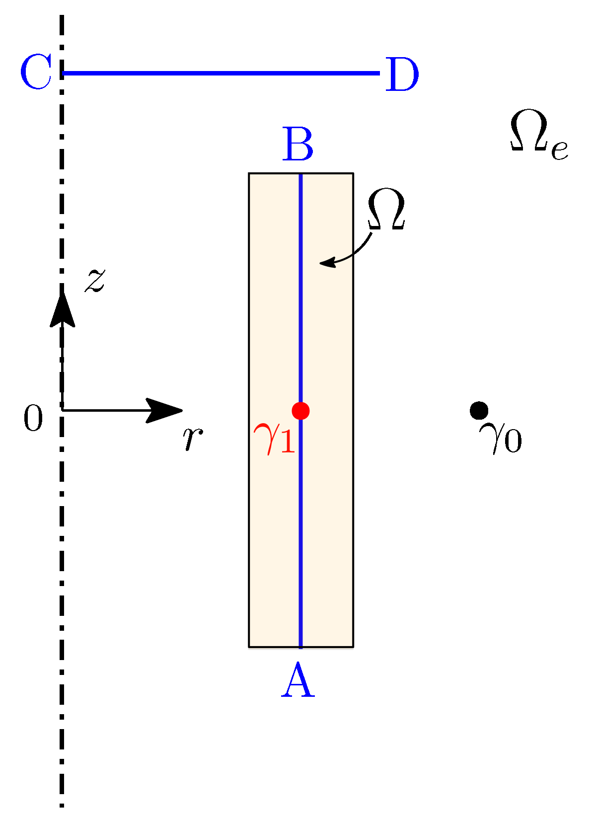
Both direct and indirect hybrid formulations are first validated by considering an axysimmetric benchmark with a highly-accurate third-order 2D FEM solution for error computation. Such a benchmark is a variant of that one presented in [14]. The model geometry is depicted in Figure 3. It consists of a conductive shell $\Omega$ (5 mm inner radius, 5 mm thick, 4 cm long, ${\mu }_r$ = 2 relative magnetic permeability, $\sigma$ = 25 MS/m electric conductivity) excited by a coaxial current loop ${\gamma }_0$ (1.5 cm radius, 1000 A current RMS value, 100 Hz frequency). For the cylindrical shell, the first Betti number is ${\beta }_1(\Omega )=1$; therefore, a unique cohomology generator is used. Such a generator, i.e., the virtual loop ${\gamma }_1$ of 7.5 mm radius, is centered at the origin of the cylindrical coordinate system in Figure 3.

The 2D FEM model is bounded by a circular region with 60 cm radius, and it was discretized by 94,120 third-order triangular elements, after refining till convergence. With the hybrid formulations, only $\Omega$ needs to be meshed. The element size was chosen to be approximately 1/5 of the skin depth, i.e., 7.11 mm at 100 Hz. The domain mesh used for the CM discretization consists of 42,125 tetrahedrons, 86,568 triangles, and 52,697 edges, with an average element size is $1.27$ mm. The unbounded domain ${\Omega }_e$ was treated with both direct and indirect BEM discretization by using a surface mesh with 4636 triangles.

The overall preprocessing, including the assembly of the Poincaré–Steklov operator (with 17.17 s CPU time), was carried out in 19.24 s CPU time. For the direct formulation, the final hybrid system, consisting of 55,016 DoFs and requiring 143.34 MB for the matrix storage, was solved by $\mathrm{TFQMR}$ solver with $\mathrm{SSOR}$ preconditioning in 26.45 s CPU time. The solution attained the fixed tolerance of ${10}^{-12}$ in 457 iterations. Comparable performance was obtained with the indirect formulation: 18.95 s CPU time for the DN map assembly, 26.25 s CPU time for the final matrix system solution with 449 iterations.

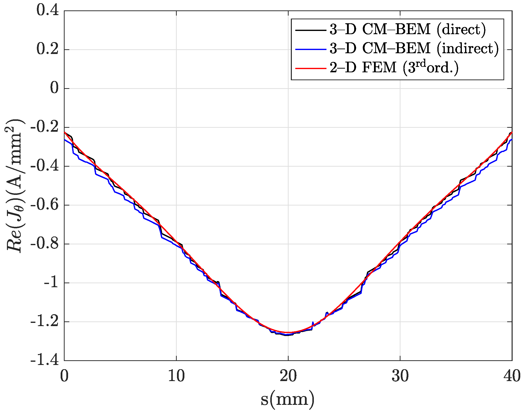
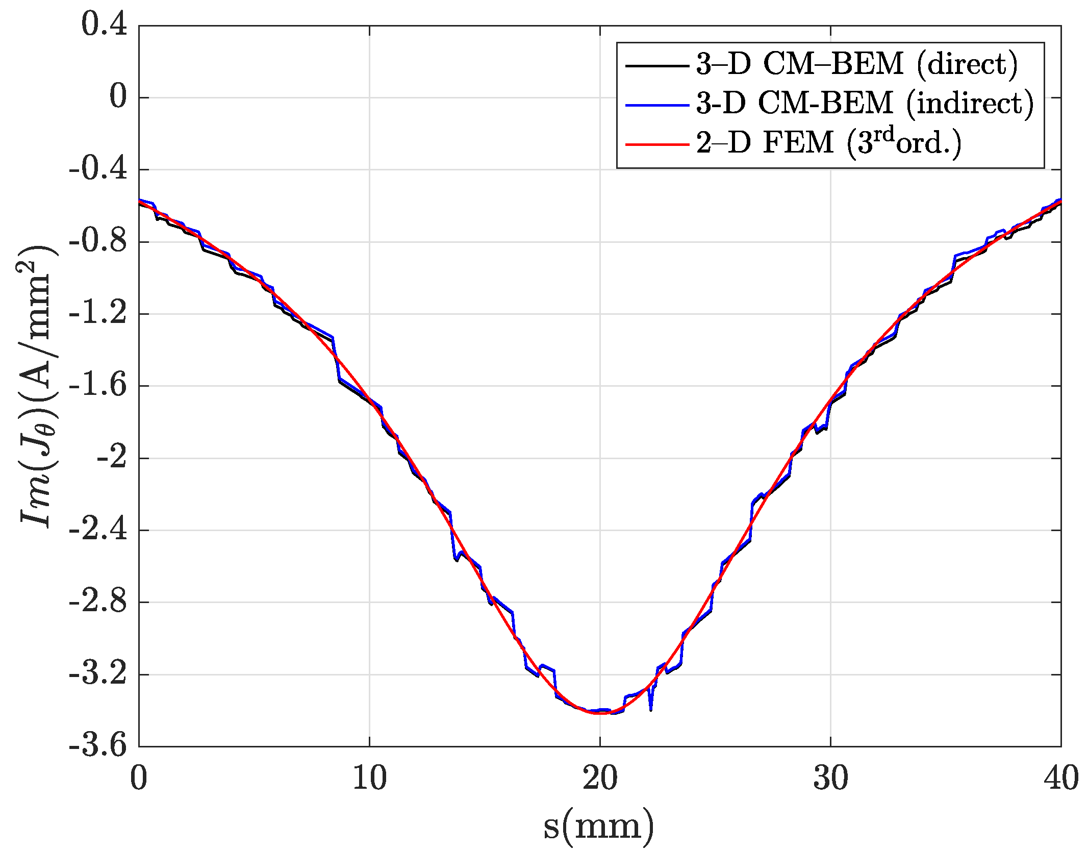
In order to check the local accuracy of both hybrid formulations, the eddy–current density was computed by both 2D FEM and CM–BEM formulations along the vertical line A-B in Figure 3, with coordinates $r=7.5$ mm, $z=\left[-20,20\right]$ mm and sampled into 401 equally spaced field points. On the 3D model for hybrid formulation, the plane $y=0$ was considered as a $r,z$ symmetry plane. The eddy–current density was obtained from the approximate electric field, expanded as in (47) with piecewise constant bases, by using the local Ohm’s law (4). Figure 4 and Figure 5 show respectively the real and the imaginary parts of the azimuthal component of the eddy–current density $J_{\theta }$. In such a case, the maximum discrepancies between the direct CM–BEM and 2D FEM results, taken as a reference, are: $3.11\%$ for the real part, $4.32\%$ for the imaginary part. Similar results were obtained for the indirect hybrid formulation: $4.47\%$ for the real part, $4.10\%$ for imaginary part.

In order to assess the convergence properties of both hybrid formulations, the eddy–current distribution in $\Omega$, computed by CM–BEM software, was compared to that one computed by third-order 2D FEM in terms of $L^2$-norm relative discrepancy, as:

$$e_J=\frac{{\parallel \mathbf{J}-{\mathbf{J}}_{\mathrm{ref}}\parallel }_{L^2(\Omega )}}{{\parallel {\mathbf{J}}_{\mathrm{ref}}\parallel }_{L^2(\Omega )}},$$

(101)

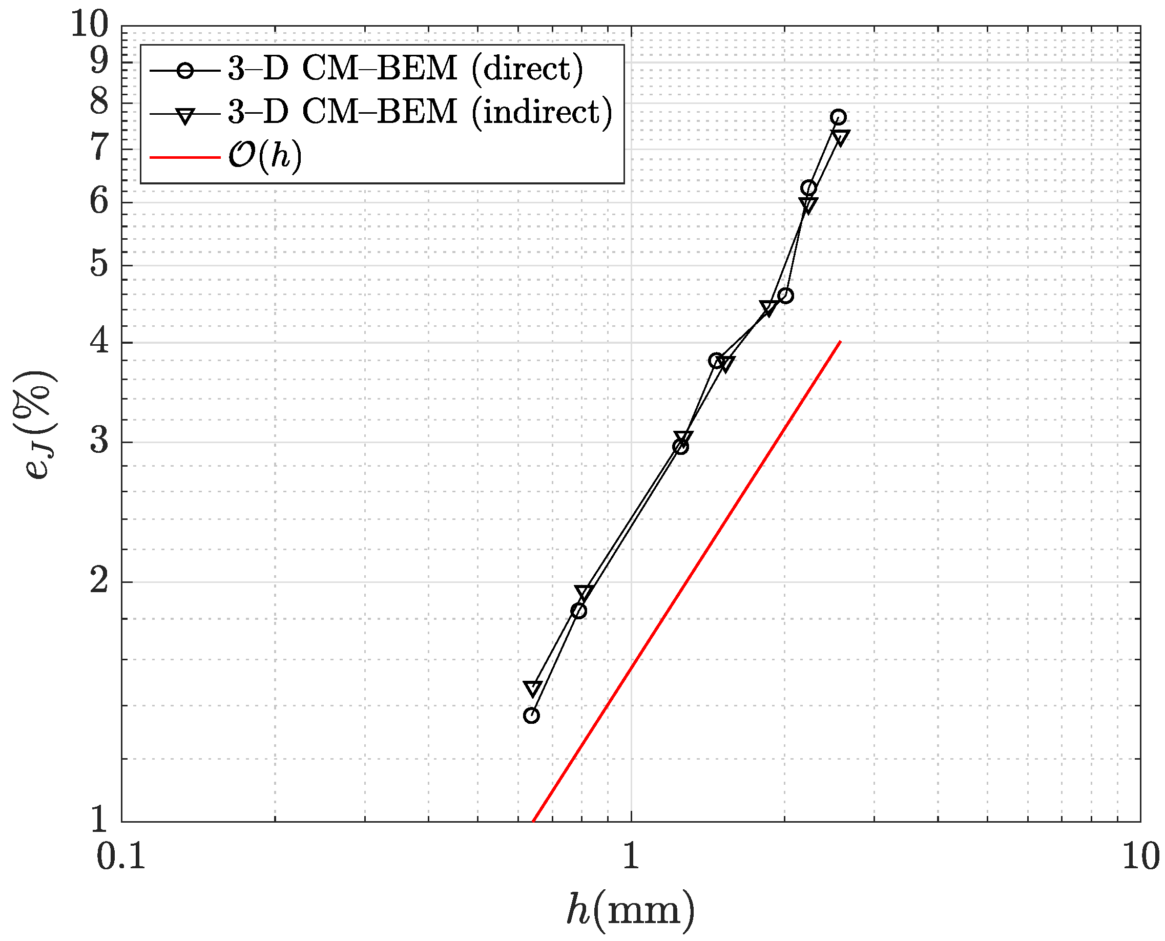
where ${\mathbf{J}}_{\mathrm{ref}}$ is the reference FEM solution, computed on a very fine rectangular grid of field points in $\Omega$. The $L^2$-norm relative error was computed by numerical integration with a 1-point Gaussian quadrature rule. Figure 6 shows the relative discrepancy for both direct and indirect formulations, evaluated for different mesh sizes. The mesh size h is defined as the maximum radius of all the spheres circumscribing tetrahedrons of the mesh. It can be observed that hybrid formulation shows similar accuracy for any mesh refinement and that the convergence behavior is linear such as first-order 3D FEM.

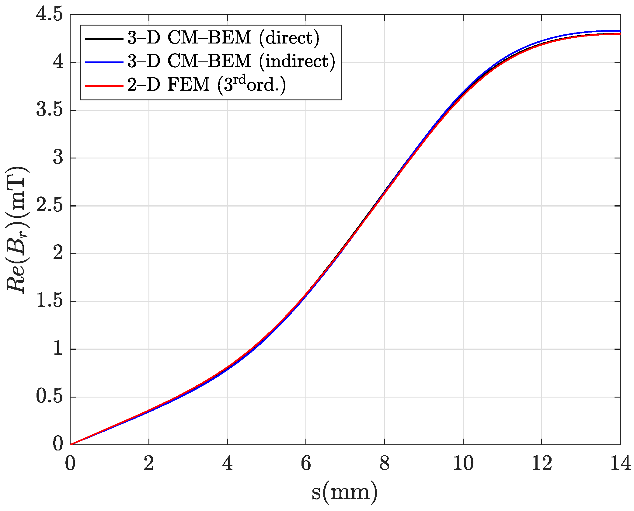
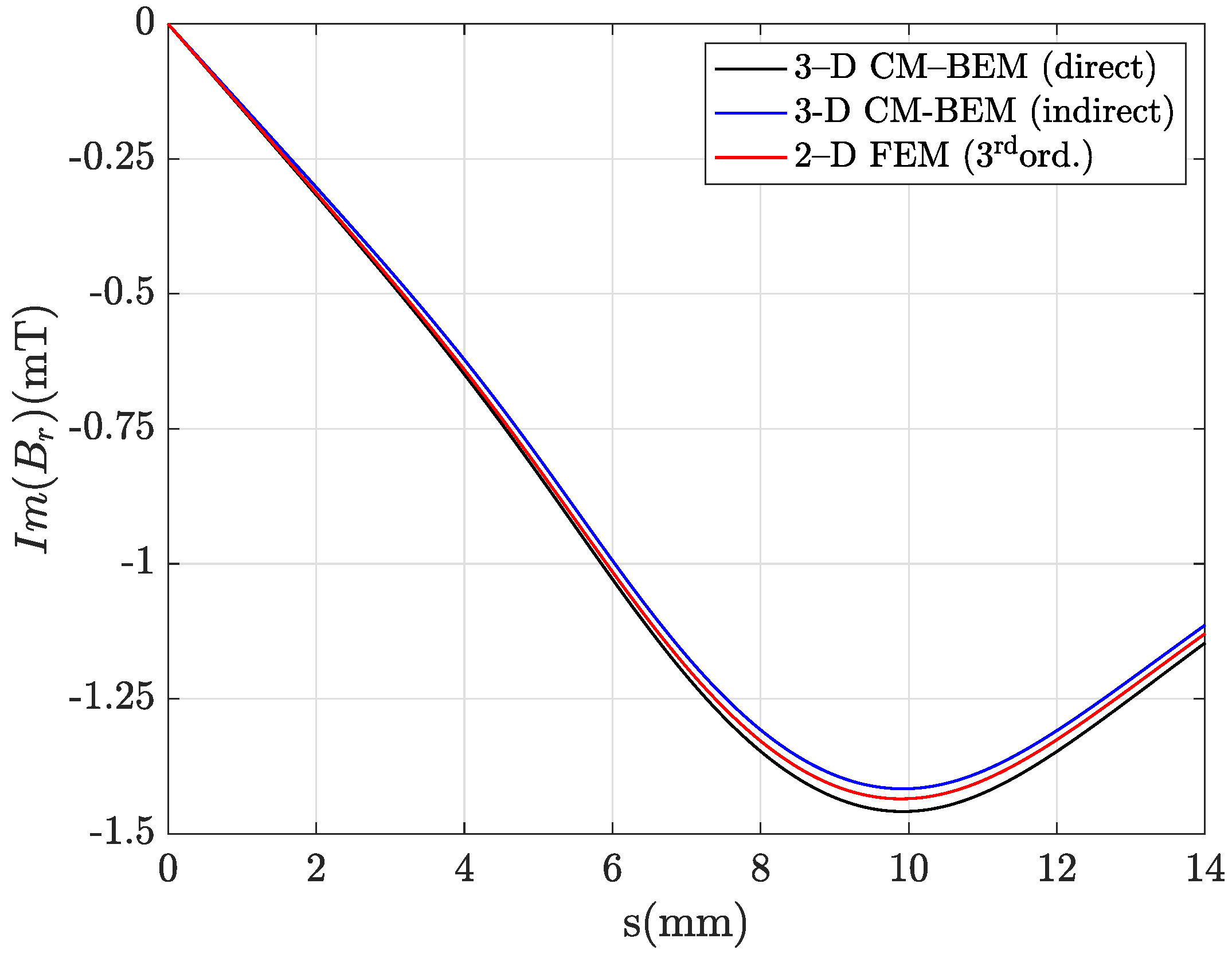
In order to check the local accuracy of both hybrid formulations in the air region, the magnetic flux density was computed along the horizontal line C-D in Figure 3, with coordinates $r=\left[0,14\right]$ mm, $z=23$ mm and sampled into 401 equally spaced field points such as line A-B. For the direct formulation, the field distribution is obtained from the numerical differentiation of ${\phi }_r$, given by (30), using a three-point stencil along any coordinate axis, i.e., six sampling points are used for any field point along the line C-D. For the indirect formulation, the field computation is fully analytical, i.e., it is obtained by combining (21) and (35), and it requires only one function evaluation per field point.

Figure 7 and Figure 8 show, respectively, the real and the imaginary parts of the radial component of the magnetic flux density $B_r$. In such a case, the maximum discrepancies between the direct CM–BEM and 2D FEM results (taken as a reference) are: $0.53\%$ for the real part, $1.67\%$ for the imaginary part. Similar values were found for the indirect formulation: $0.94\%$ for the real part, $1.46\%$ for the imaginary part. Figure 9 and Figure 10 show the same comparisons for the axial field component $B_z$. Maximum discrepancies are in that case: $0.33\%$ for the real part, $1.43\%$ for the imaginary part (direct formulation); $0.89\%$ for the real part, $2.07\%$ for the imaginary part (indirect formulation). It is interesting to observe that, for any field component, numerical results show a complementary behavior, with hybrid formulation values bilaterally bounding FEM reference values.

6.2. Bath Plate

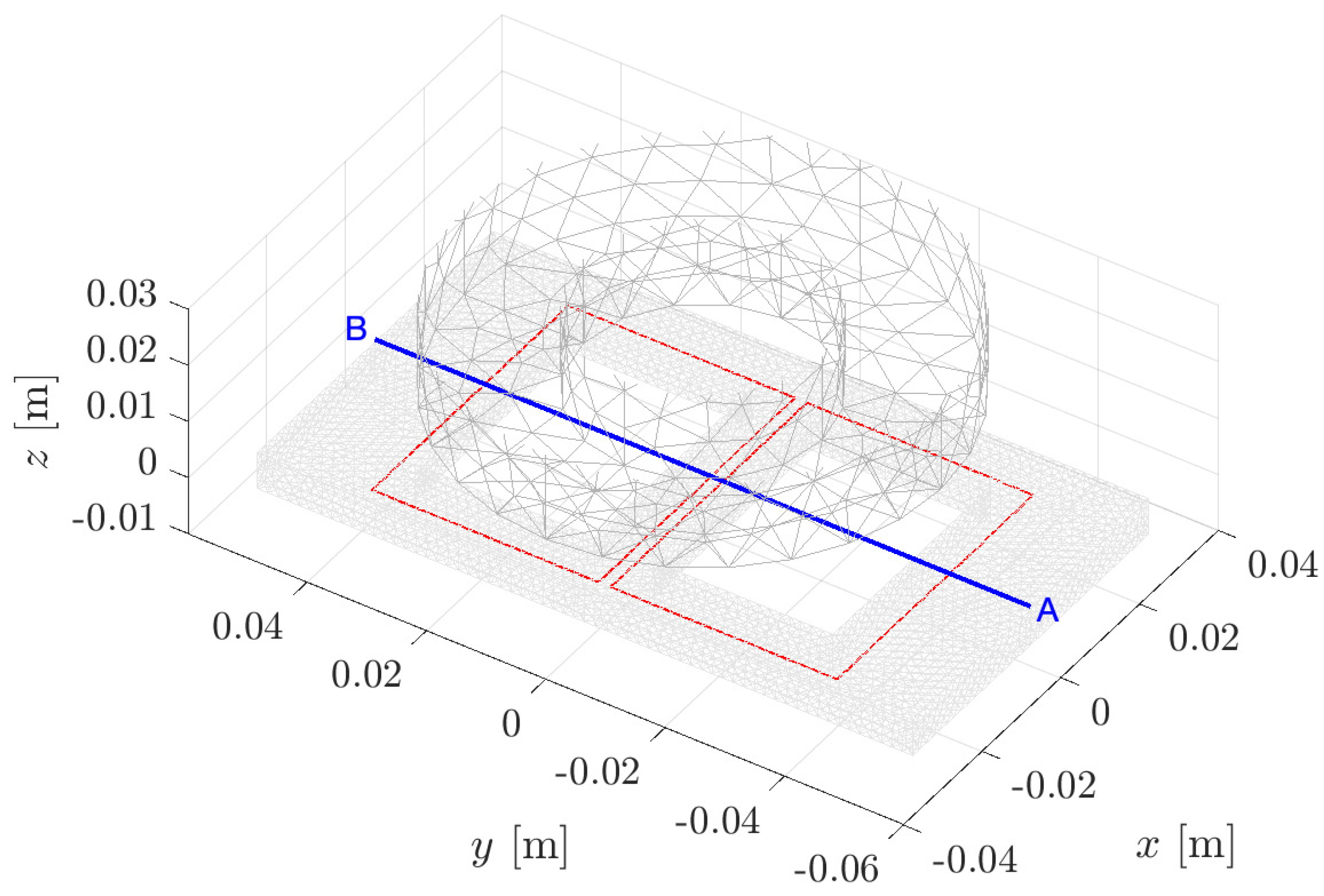
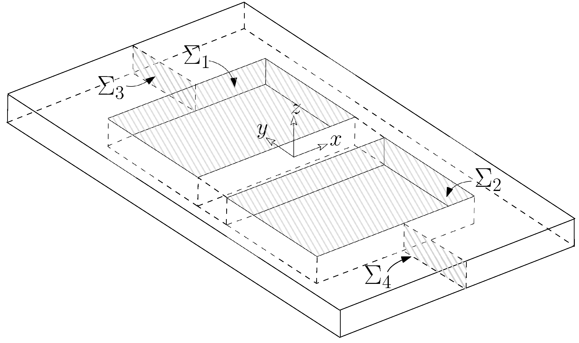
The Bath Plate problem consists of a conducting plate $\Omega$ (32.78 MS/m electrical conductivity, ${\mu }_r=1$ relative magnetic permeability, 6.35 mm thick, 60 mm wide, 110 mm long) excited by an AC current–driven cylindrical coil ${\Omega }_0$ (1240 A RMS current, 20 mm inner radius, 40 mm outer radius, 20 mm thick, located 15 mm above the plate) at two different frequencies (50 Hz, 200 Hz). The origin of the Cartesian coordinate system $(x,y,z)$ is centered on the plate surface; the coil vertical axis is the z-axis. Two holes with square cross-section (40 mm × 30 mm) are centered on $x=0$, $y=\pm 20$ mm; therefore, the conducting domain $\Omega$ is multiply connected, with ${\beta }_1(\Omega )=2$. Figure 11 shows the CM–BEM model, with virtual loops ${\gamma }_{\pm }$ (rectangular coils, 50 mm × 38 mm, centered at $x=0$, $y=\pm 55$ mm, $z=-3$ mm, in red) and the line A-B used for comparing magnetic flux density distributions ($x=0$ mm, $y=[-55,55]$ mm, $z=0.5$ mm, in blue). Such a horizontal line was discretized into 401 equally spaced field points.

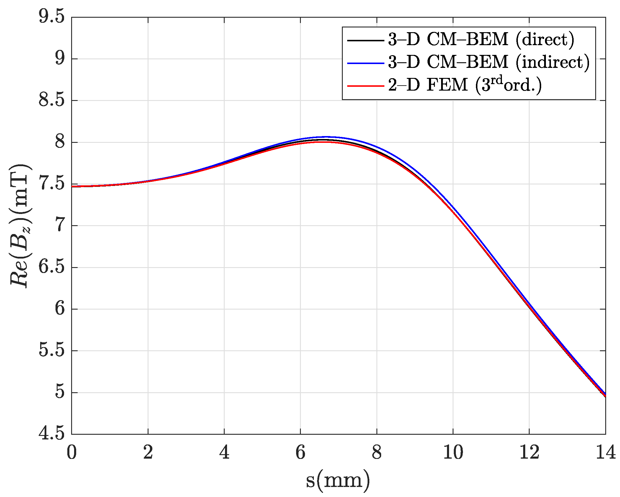
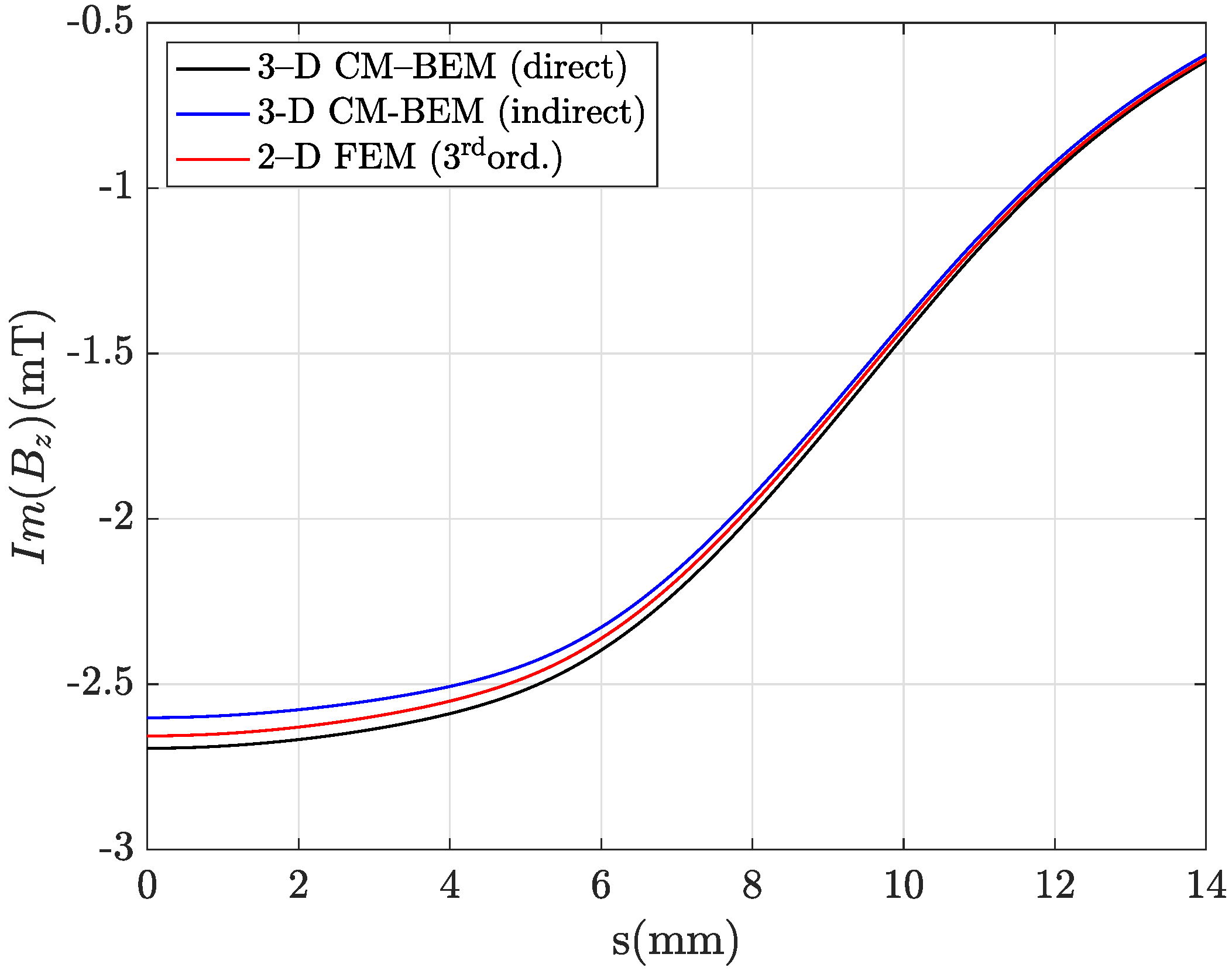
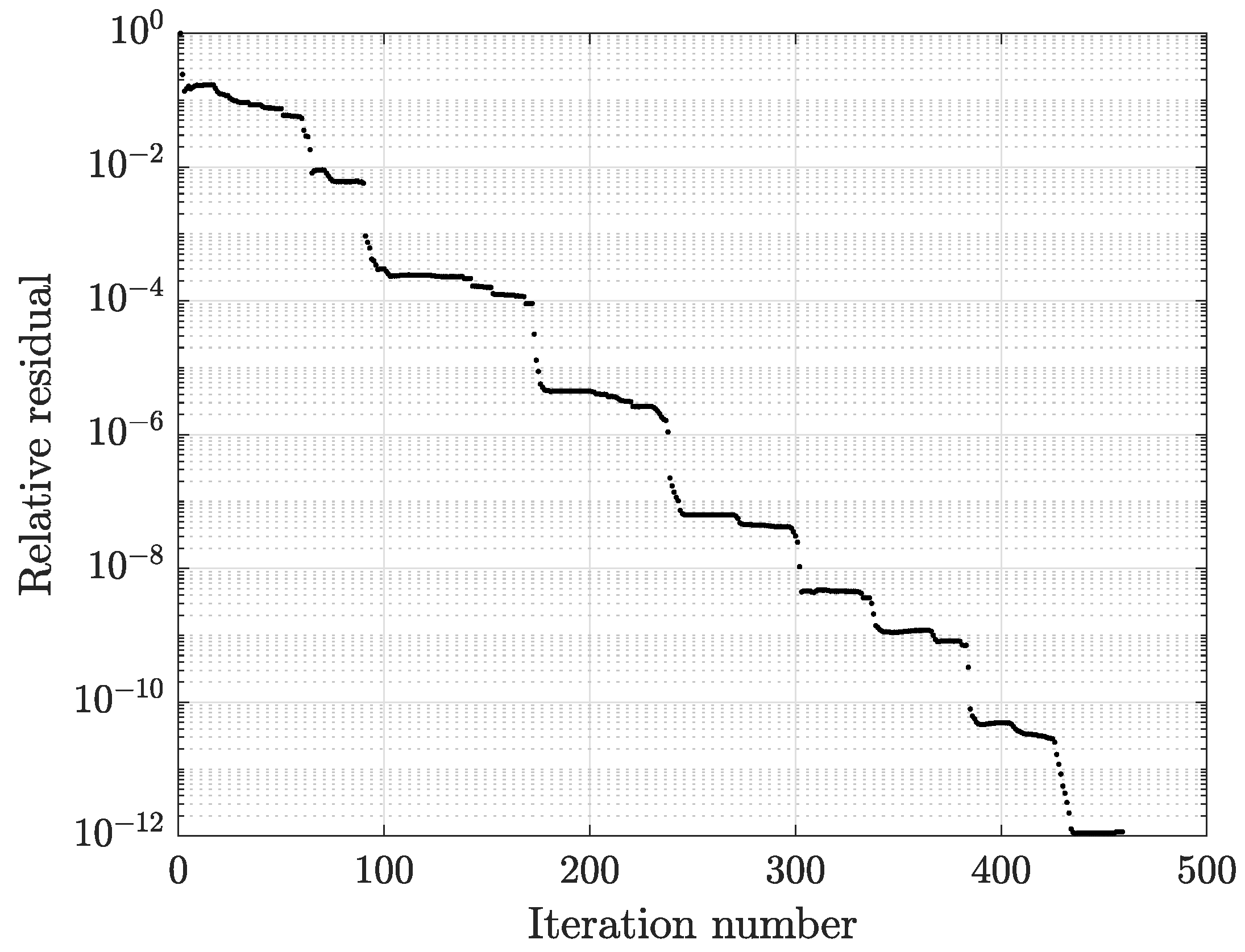
To examine the accuracy of 3D CM–BEM results (indirect formulation), the real and imaginary parts of the z-component of the magnetic flux density were computed, for both frequency values, along the line A-B. For the sake of comparison, numerical results from a second-order 3D FEM, based on a classical A–A formulation, were used. For 3D CM–BEM, $\Omega$ was discretized into l69,492 tetrahedrons, with mesh size $h=1.45$ mm (smaller than conductor skin depth at 200 Hz, i.e, 6.22 mm), 88,443 edges, and 143,798 faces (among these, 9628 were on the interface $\Gamma =\partial \Omega$). ${\Omega }_0$ was discretized into 1764 tetrahedrons. Unlike the hybrid method, 3D FEM required a bounding box (a cube of 1 m side, centered at the origin) on which magnetic wall BCs were applied. In order to get a reference solution, the 3D FEM discretization was refined up to convergence (80,862 second-order tetrahedrons were used). In particular, $\Omega$ was discretized into 5249 tetrahedrons, with 2 mm maximum element size. Note that, with FEM, only a half of the problem was considered due to symmetry. The A–A formulation needs to introduce a fake conductivity in the air region (0.1 S/m) for the final matrix system regularization. This correction, which was not required by the CM-BEM, introduced an approximation in the numerical results. A 3D FEM model (517,341 DOFs, 3.51 GB RAM) was solved by $\mathrm{TFQMR}$ solver with geometric multigrid preconditioning in 54 s CPU time (at 50 Hz) and in 48 s (at 200 Hz) to attain a ${10}^{-12}$ tolerance. Preprocessing of CM–BEM required 190.25 s CPU time, including the computation of source field, the assembly of both CM and BEM matrices, and RHS vectors. Most of the computing time was required for computation of the DN map (size 9628, computed in 88.82 s CPU time) and RHS vectors with Biot–Savart’s integration (computed in 95.75 s). Note that only 14.23 seconds of CPU time were required for matrix inversion when building the DN map. The iterative solution by $\mathrm{TFQMR}+\mathrm{SSOR}$ solver of the CM–BEM final system (with 89,997 DOFs, 565.09 MB RAM) required 93.25 s CPU time, with 459 iterations, to attain ${10}^{-12}$ tolerance (50 Hz) and 69.18 s, with 324 iterations (200 Hz). For instance, Figure 12 shows that the solver convergence pattern at 50 Hz, which is smooth and linear. A similar behavior for TFQMR was found at 200 Hz.

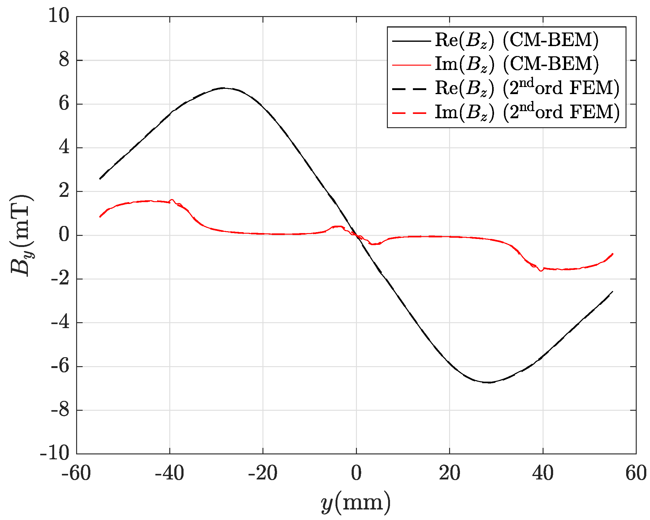
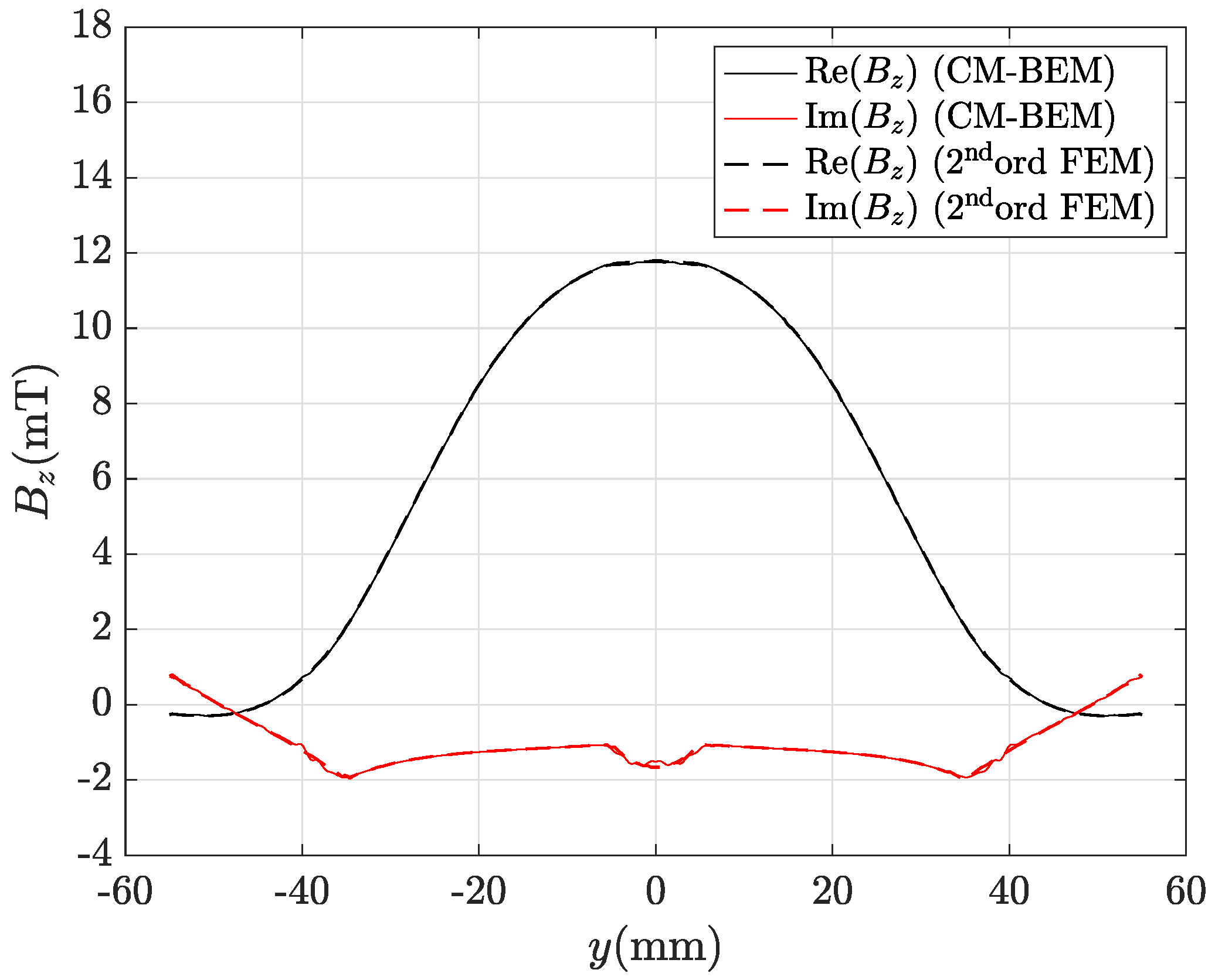
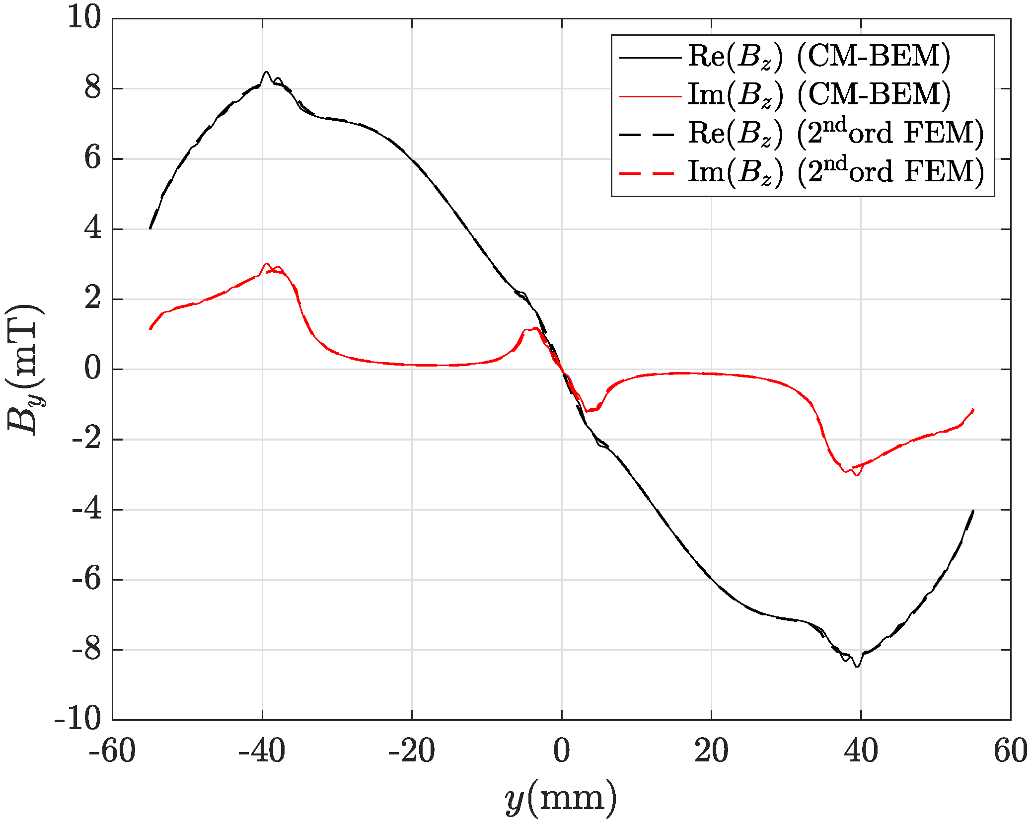
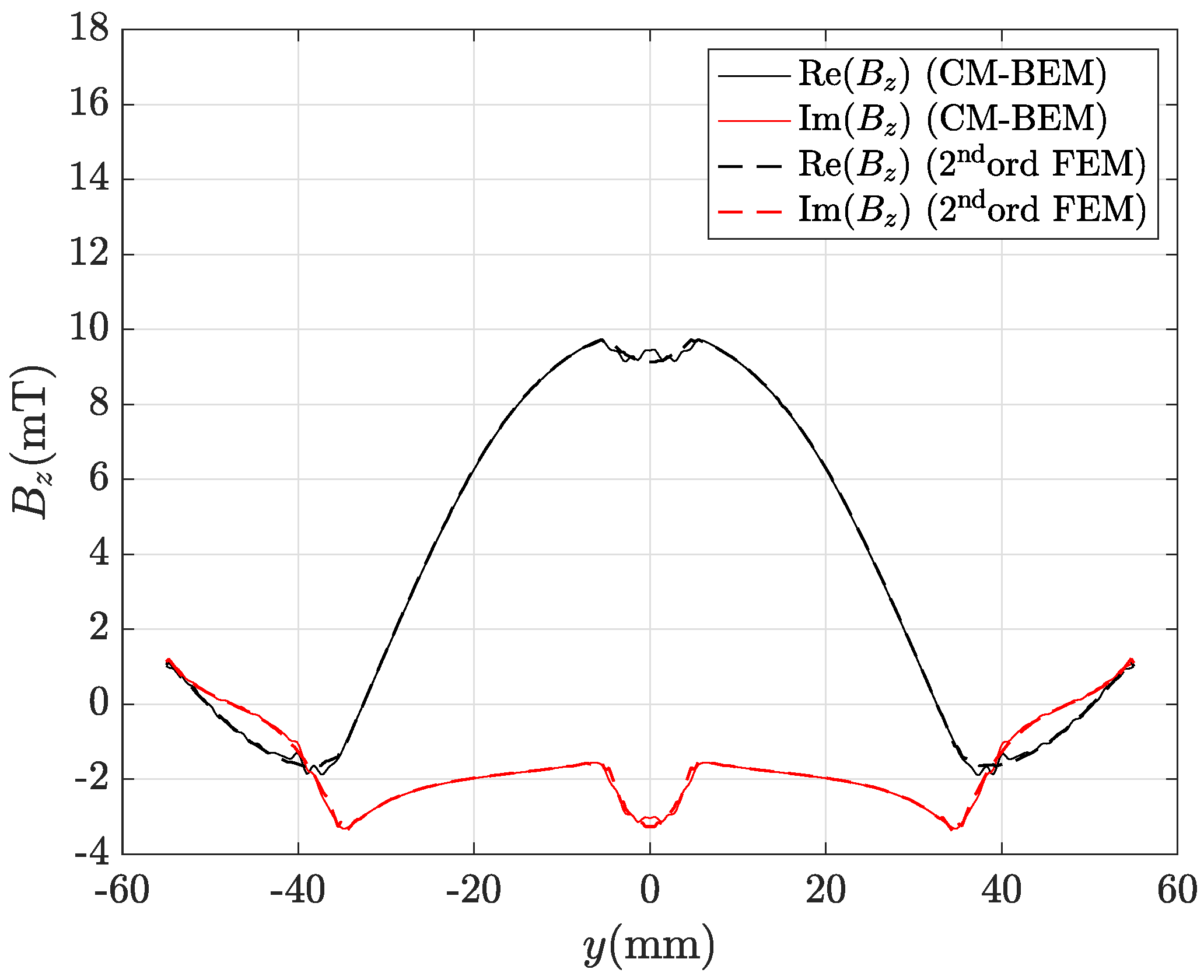
The y-axis and z-axis magnetic flux density components were evaluated along the horizontal line A-B of Figure 11 by both 3D CM–BEM and 3D FEM on 401 equally spaced points. Figure 13 and Figure 14 show that field profiles at 50 Hz are in very good agreement. The maximum discrepancies from 3D FEM, for the real and imaginary parts of $B_y$, are, respectively, $0.98\%$ and $11.52\%$, whereas, for $B_z$, they are $0.60\%$ and $8.81\%$, respectively. Therefore, even by using a relatively coarse mesh refinement for CM–BEM, a good agreement with second-order FEM is obtained. Similar results were found at 200 Hz: $4.42\%$ and $9.83\%$, respectively, for real and the imaginary part of $B_y$ (Figure 15), $3.72\%$ and $9.36\%$, respectively, for the real and the imaginary part of $B_z$ (Figure 16).

The global quantities considered in the benchmark were the magnetic fluxes through the plate holes (cut surfaces ${\Sigma }_1$ and ${\Sigma }_2$, on the plane $z=0$, in Figure 17) and the eddy–currents through the plate ribs (cut surfaces ${\Sigma }_3$ and ${\Sigma }_4$, on the plane $x=0$, in Figure 17). Magnetic fluxes ${\Phi }_{{\Sigma }_1}={\int }_{{\Sigma }_1}\mathbf{B}·{\mathbf{e}}_{z}d\Sigma$, ${\Phi }_{{\Sigma }_2}={\int }_{{\Sigma }_2}\mathbf{B}·{\mathbf{e}}_{z}d\Sigma$, with ${\mathbf{e}}_z$ unit vector along the z-axis, were computed by both 3D CM–BEM and second-order FEM through ${\Sigma }_1$ and ${\Sigma }_2$. The same comparisons were carried out for current phasors $I_{{\Sigma }_3}={\int }_{{\Sigma }_3}\mathbf{J}·{\mathbf{e}}_{x}d\Sigma$, $I_{{\Sigma }_4}={\int }_{{\Sigma }_4}\mathbf{J}·{\mathbf{e}}_{x}d\Sigma$ through ${\Sigma }_3$ and ${\Sigma }_4$, with ${\mathbf{e}}_x$ unit vector along the x-axis. Due to model symmetry, relationships ${\Phi }_{{\Sigma }_1}={\Phi }_{{\Sigma }_2}$ and $I_{{\Sigma }_3}=-I_{{\Sigma }_4}$ theoretically hold. Fluxes were computed by assuming a piecewise constant approximation of both $\mathbf{B}$ and $\mathbf{J}$ fields for the CM-BEM model, and a fourth-order quadrature scheme for 3D FEM.

Table 1. Real and imaginary parts of magnetic flux (μWb) computed through cut surfaces ${\Sigma }_1,{\Sigma }_2$ by 3D CM–BEM and 3D FEM (2nd order) at 50 Hz and 200 Hz frequency.

		$\mathit{R}\mathit{e}\left({\mathbf{\Phi }}_{{\mathbf{\Sigma }}_1}\right)$	$\mathit{I}\mathit{m}\left({\mathbf{\Phi }}_{{\mathbf{\Sigma }}_1}\right)$	$\mathit{R}\mathit{e}\left({\mathbf{\Phi }}_{{\mathbf{\Sigma }}_2}\right)$	$\mathit{I}\mathit{m}\left({\mathbf{\Phi }}_{{\mathbf{\Sigma }}_2}\right)$
50 Hz	3D CM–BEM	$7.869$	$-1.958$	$7.872$	$-1.958$
	FEM (2nd ord.)	$7.862$	$-1.974$	$7.862$	$-1.974$
200 Hz	3D CM–BEM	$4.435$	$-3.126$	$4.438$	$-3.127$
	FEM (2nd ord.)	$4.394$	$-3.142$	$4.394$	$-3.142$

shows that real and imaginary parts of magnetic fluxes, computed by 3D CM–BEM, are in good agreement with reference values obtained with second-order FEM at 50 Hz and 200 Hz. Similar considerations apply to eddy–current values through surfaces ${\Sigma }_3$ and ${\Sigma }_4$ reported in

Table 2. Real and imaginary parts of eddy–current (A) computed through cut surfaces ${\Sigma }_3,{\Sigma }_4$ by 3D CM–BEM and 3D FEM (2nd) at 50 Hz and 200 Hz frequency.

		$\mathit{R}\mathit{e}\left({\mathit{I}}_{{\mathbf{\Sigma }}_3}\right)$	$\mathit{I}\mathit{m}\left({\mathit{I}}_{{\mathbf{\Sigma }}_3}\right)$	$\mathit{R}\mathit{e}\left({\mathit{I}}_{{\mathbf{\Sigma }}_4}\right)$	$\mathit{I}\mathit{m}\left({\mathit{I}}_{{\mathbf{\Sigma }}_4}\right)$
50 Hz	3D CM–BEM	$21.811$	$63.412$	$-21.819$	$-63.080$
	FEM (2nd ord.)	$21.766$	$63.258$	$-21.765$	$-63.259$
200 Hz	3D CM–BEM	$133.941$	$98.886$	$-133.687$	$-97.393$
	FEM (2nd ord.)	$133.550$	$98.518$	$-133.540$	$-98.529$

. Note that $I_{{\Sigma }_3}$, $I_{{\Sigma }_4}$ can be also obtained from the CM–BEM final matrix system solution. In fact, according to Ampère’s law applied along boundaries $\partial {\Sigma }_3$ and $\partial {\Sigma }_4$, these coincide with currents flowing along virtual loops in Figure 11. With a counterclockwise orientation of ${\gamma }_{\pm }$, currents of virtual loops, obtained from the solution of (100), are $I_{{\gamma }_{+}}=-21.797-ı63.378$ and $I_{{\gamma }_{-}}=-21.794-ı63.366$, at 50 Hz, and $I_{{\gamma }_{+}}=-133.669-ı98.802$, $I_{{\gamma }_{-}}=-133.645-ı98.778$, at 200 Hz. It can be noted that real and imaginary values of $I_{{\gamma }_{\pm }}$ are in very good agreement with values in Table 2.

7. Conclusions

Several hybrid approaches based on the CM, which is a valid alternative to the FEM, have been presented under a unified theoretical framework. It has been shown that, by introducing an augmented dual grid in the CM discretization process, novel interface topological operators can be obtained. These operators can be used in order to construct symmetric (direct and indirect) hybrid formulations, which result in final matrix systems amenable to iterative solution. Numerical tests show that direct and indirect approaches have similar accuracy. As an example of application, the indirect formulation has been tested on a realistic 3D eddy–current problem, showing the same degree of accuracy of second-order FEM but with much less DOFs used for the discretization.

References

- Chen, Q.; Konrad, A. A review of finite element open boundary techniques for static and quasi-static electromagnetic field problems. IEEE Trans. Magn. 1997, 33, 663–676. [Google Scholar] [CrossRef]
- Bossavit, A. Computational Electromagnetism: Variational Formulations, Complementarity, Edge Elements; Academic Press: San Diego, CA, USA, 1998. [Google Scholar] [CrossRef]
- Tonti, E. A Direct Discrete Formulation of Field Laws: The Cell Method. Comput. Model. Eng. Sci. 2001, 2, 237–258. [Google Scholar]
- Tonti, E. Why starting from differential equations for computational physics? J. Comput. Phys. 2014, 257, 1260–1290. [Google Scholar]
- Codecasa, L.; Minerva, V.; Politi, M. Use of barycentric dual grids for the solution of frequency domain problems by FIT. IEEE Trans. Magn. 2004, 40, 1414–1419. [Google Scholar]
- Codecasa, L.; Politi, M. Explicit, Consistent, and Conditionally Stable Extension of FD-TD to Tetrahedral Grids by FIT. IEEE Trans. Magn. 2008, 44, 1258–1261. [Google Scholar]
- Codecasa, L.; Trevisan, F. Constitutive equations for discrete electromagnetic problems over polyhedral grids. J. Comput. Phys. 2007, 225, 1894–1918. [Google Scholar]
- Giuffrida, C.; Gruosso, G.; Repetto, M. Finite formulation of nonlinear magnetostatics with Integral boundary conditions. IEEE Trans. Magn. 2006, 42, 1503–1511. [Google Scholar]
- Gruosso, G.; Repetto, M. Magnetostatic solution by hybrid technique and fast multipole method. Phys. B Condens. Matter 2008, 403, 368–371. [Google Scholar]
- Alotto, P.; Gruosso, G.; Moro, F.; Repetto, M. A Boundary Integral Formulation for Eddy Current Problems Based on the Cell Method. IEEE Trans. Magn. 2008, 44, 770–773. [Google Scholar]
- Codecasa, L. Refoundation of the Cell Method Using Augmented Dual Grids. IEEE Trans. Magn. 2014, 50, 497–500. [Google Scholar]
- Moro, F.; Codecasa, L. Indirect Coupling of the Cell Method and BEM for Solving 3D Unbounded Magnetostatic Problems. IEEE Trans. Magn. 2016, 52. [Google Scholar]
- Moro, F.; Codecasa, L. A 3D Hybrid Cell Method for Induction Heating Problems. IEEE Trans. Magn. 2017, 53, 1–4. [Google Scholar]
- Moro, F.; Codecasa, L. A 3D Hybrid Cell Boundary Element Method for Time-Harmonic Eddy Current Problems on Multiply Connected Domains. IEEE Trans. Magn. 2019, 55. [Google Scholar]
- Hiptmair, R.; Ostrowski, J. Coupled boundary-element scheme for eddy-current computation. J. Eng. Math. 2005, 51, 231–250. [Google Scholar]
- Rodríguez, A.A.; Bertolazzi, E.; Ghiloni, R.; Valli, A. Construction of a Finite Element Basis of the First de Rham Cohomology Group and Numerical Solution of 3D Magnetostatic Problems. SIAM J. Numer. Anal. 2013, 51, 2380–2402. [Google Scholar]
- Hiptmair, R.; Sterz, O. Current and voltage excitations for the eddy–current model. Int. J. Numer. Model. Electron. Netw. Devices Fields 2005, 18, 1–21. [Google Scholar]
- Folland, G. Introduction to Partial Differential Equations; Princeton University Press: Princeton, NJ, USA, 1995. [Google Scholar]
- Brebbia, C.; Butterfield, R. Formal equivalence of direct and indirect boundary element methods. Appl. Math. Model. 1978, 2, 132–134. [Google Scholar] [CrossRef]
- Rucker, W.M.; Richter, K.R. Three-dimensional magnetostatic field calculation using boundary element method. IEEE Trans. Magn. 1988, 24, 23–26. [Google Scholar] [CrossRef]
- Ren, Z.; Bouillault, F.; Razek, A.; Vérité, J. Comparison of different boundary integral formulations when coupled with finite elements in three dimensions. IEE Proc. (Phys. Sci. Meas. Instrum. Manag. Educ. Rev.) 1988, 135, 501–507. [Google Scholar] [CrossRef]
- Graciani, E.; Mantič, V.; París, F.; Cañas, J. A critical study of hypersingular and strongly singular boundary integral representations of potential gradient. Comput. Mech. 2000, 25, 542–559. [Google Scholar] [CrossRef]
- Costabel, M. Principles of boundary element methods. Comput. Phys. Rep. 1987, 6, 243–274. [Google Scholar] [CrossRef]
- Andjelic, Z.; Of, G.; Steinbach, O.; Urthaler, P. Boundary element methods for magnetostatic field problems: A critical view. Comput. Vis. Sci. 2011, 14, 117–130. [Google Scholar] [CrossRef]
- Moro, F.; Smajic, J.; Codecasa, L. A Novel h–φ Approach for Solving Eddy–Current Problems in Multiply Connected Regions. IEEE Access 2020, 8, 170659–170671. [Google Scholar] [CrossRef]
- Moro, F.; Codecasa, L. Domain Decomposition With Non-Conforming Polyhedral Grids. IEEE Access 2021, 9, 1465–1481. [Google Scholar] [CrossRef]
- Zhou, P.B. Numerical Analysis of Electromagnetic Fields; Springer: Berlin/Heidelberg, Germany, 1993. [Google Scholar]
- Bossavit, A.; Vérité, J. The “TRIFOU” Code: Solving the 3D eddy-currents problem by using H as state variable. IEEE Trans. Magn. 1983, 19, 2465–2470. [Google Scholar] [CrossRef]
- Rodger, D. Benchmark problem 3 (the Bath Plate). COMPEL 1988, 7, 47–63. [Google Scholar]
Short Biography of Authors