
Alternative Dirichlet Priors for Estimating Entropy via a Power Sum Functional


1
Department of Statistics, Faculty of Natural and Agricultural Sciences, University of Pretoria, Pretoria 0028 , South Africa
2
Centre of Excellence in Mathematical and Statistical Science, University of Witwatersrand, Johannesburg 2050, South Africa
*
Author to whom correspondence should be addressed.
†
These authors contributed equally to this work.
Mathematics 2021, 9(13), 1493; https://0-doi-org.brum.beds.ac.uk/10.3390/math9131493
Submission received: 29 May 2021
/
Revised: 20 June 2021
/
Accepted: 23 June 2021
/
Published: 25 June 2021
(This article belongs to the Special Issue Advances in Mathematics and Statistics with Applications in Engineering and Industry)
Abstract
:Entropy is a functional of probability and is a measurement of information contained in a system; however, the practical problem of estimating entropy in applied settings remains a challenging and relevant problem. The Dirichlet prior is a popular choice in the Bayesian framework for estimation of entropy when considering a multinomial likelihood. In this work, previously unconsidered Dirichlet type priors are introduced and studied. These priors include a class of Dirichlet generators as well as a noncentral Dirichlet construction, and in both cases includes the usual Dirichlet as a special case. These considerations allow for flexible behaviour and can account for negative and positive correlation. Resultant estimators for a particular functional, the power sum, under these priors and assuming squared error loss, are derived and represented in terms of the product moments of the posterior. This representation facilitates closed-form estimators for the Tsallis entropy, and thus expedite computations of this generalised Shannon form. Select cases of these proposed priors are considered to investigate the impact and effect on the estimation of Tsallis entropy subject to different parameter scenarios.
1. Introduction
Shannon entropy and related information measures are functionals of probability and a measurement of information contained in a system that arise in information theory, machine learning and text modelling, amongst others. Ref. [1] discussed quantifying the information carried by neural signals to estimating the dependency structure and inferring causal relations, uncertainty and dispersion in statistics being applied in fields such as molecular biology. Other interests include studies measuring complexity of dynamics in physics, to studies measuring diversity in ecology and genetics, fields of coding theory and cryptography [2], financial analysis and data compression [3]. Numerous inferential tasks rely on data-driven procedures to estimate these quantities. In these settings and utilising the estimated quantities, researchers are often confronted with data arising from an unknown discrete distribution, and seek to estimate its entropy. This motivates sustained research interest within entropy, coupled with the current data-driven and computing-rich era, for practitioners.
Entropy estimation remains an openly discussed challenge. Ref. [4] investigated how the maximum likelihood estimator (MLE) performed. This is also referred to as the plug-in principle in functional estimation, where a point estimate of the parameter is used to build an estimate for a functional of the parameter. The classical asymptotic theory of MLEs does not adequately address high-dimensional settings in this current data-driven era [4]. High-dimensional statistics arguably demand theoretical tools to address the needs of these high-dimensional settings. Ref. [5] investigated 18 different estimation measures and the suitability was determined experimentally based on the bias and the mean squared error. This work takes a Bayesian approach to entropy estimation, building upon work by [1,4,6,7].
Multivariate count data constrained to add up to a certain constant are commonly modelled using the multinomial distribution. This is widely used in modelling categorical data, of which features could be for example, words in the case of textual documents or visual words in the case of images. The Dirichlet distribution, closely related to the probabilistic behaviour of the multinomial distribution, is a conjugate prior for the multinomial distribution when a Bayes perspective is of interest. Ref. [8] highlights how the use of prior distributions in a Bayesian framework makes it possible to work with very limited data sets. Ref. [9] underscores the superior performance by using the hierarchical approach which introduces the construction of the statistical model. Some meaningful studies include [1,4,6,10]. Ref. [11] also showed how using different Dirichlet distributions for the bivariate case gives one the opportunity to include prior information and expert opinion to obtain more realistic results in certain situations. Ref. [4] also experimented with the estimation of entropy and this triggered more exploration with alternative priors. Experimentation on diverse data sets might necessitate parameter-rich priors; therefore, this study proposes these alternative Dirichlet priors to address this potential challenge.
The paper illustrates how a Bayesian approach is applied in a multinomial-Dirichlet family setup, which allows us to obtain a posterior distribution from where explicit expressions for the Tsallis entropy can be derived, by particularly focussing on the Product moment for the power sum functional, and assuming squared error loss. The first of two main contributions of this paper is the addition of flexible priors from a Dirichlet family, utilising them within an information-theoretical world, which also allows for positive correlation in addition to the usual negative correlation characteristic. The second shows that using elegant constructs of the complete product moments of the posteriors, gives one the comparative advantage of obtaining explicit estimators for entropy under these Dirichlet priors. Ref. [8] echos how the computation on moments accelerates the estimation of entropy.
The paper is outlined as follows. In Section 2, the essential components that are used in the paper are outlined. In Section 3, alternative Dirichlet priors will be introduced and studied, as candidates for the Bayesian analysis of entropy. In Section 4, analytical expressions for the entropy expressions under consideration will be derived and studied. Section 5 contains conclusions and final thoughts.
2. Essential Components
The countably discrete model under consideration in this paper is given by the well-motivated multinomial distribution. A discrete random variable follows the multinomial distribution of order K (i.e., with K distinct classes of interest) with parameters and if its probability mass function (pmf) is given by
The Dirichlet distribution (of type 1, see [12]) of order and parameters for , has a probability density function (pdf) with respect to the Lebesgue measure on the Euclidean space given by
on the K dimensional simplex, defined by
and where denotes the usual gamma function (the space and constraints of this K dimensional simplex is denoted by ).
To derive a Bayesian engine, we need the likelihood function in addition to a suitable prior distribution . The fundamental relationship between the likelihood function and the prior distribution to form the posterior distribution is given by
The most popular form of entropy is that of Shannon:
Various generalised cases of this entropy exist, which relies on the power sum:
where . The power sum functional occurs in various operational problems ([4]). Under the assumption of squared error loss within Bayes estimation, the estimates of both these quantities is given by their expected values:
and
Thus, it is of value to consider the expected value of for all values of i.
Since there are cases, such as the non-extensive system like alignment processing, namely registration, which has complex behaviours associated with the phenomena of radar-imaging systems [13])which cannot be fully explained by Shannon entropy, other generalized forms were designed. The Tsallis entropy considered in this paper, which is a popular generalised entropy, tends to Shannon entropy as tends to 1 [14] and is given by
The estimate of this generalisation can be written in terms of the estimate of the power sum:
Since the power sum is easier to estimate than the Shannon entropy, the power sum is used in our case. We consider the estimate as the expectation under the posterior distribution, thus under squared-error loss.
3. Alternative Dirichlet Priors
In this section, two previously unconsidered Dirichlet priors, namely the Dirichlet generator prior and the noncentral Dirichlet prior will be proposed. Positive correlation can be observed for special cases of the Dirichlet generator prior, which is a benefit of this generator form. These new contributions add to the field of generative models for count data and have not been previously considered for entropy.
3.1. Dirichlet Generator Prior
In this section, Dirichlet generator distributions are proposed as alternative candidates. From this form, numerous flexible candidates can be “generated”.
Definition 1.
Suppose is Dirichlet-generator distributed. Then, its pdf is given by
with C a normalising constant such that
The vector is thus a Dirichlet generator variate with parameters , , and whichever additional parameters imposed, which ensures that the pdf is non-negative. The following conditions also apply:
- (1)
- is a Borel-measurable function;
- (2)
- admits a Taylor series expansion;
- (3)
- .
For illustration of the implementation of the Dirichlet generator prior, we focus on
where denotes the generalised hypergeometric function (see [15]) and is the Pochhammer function.
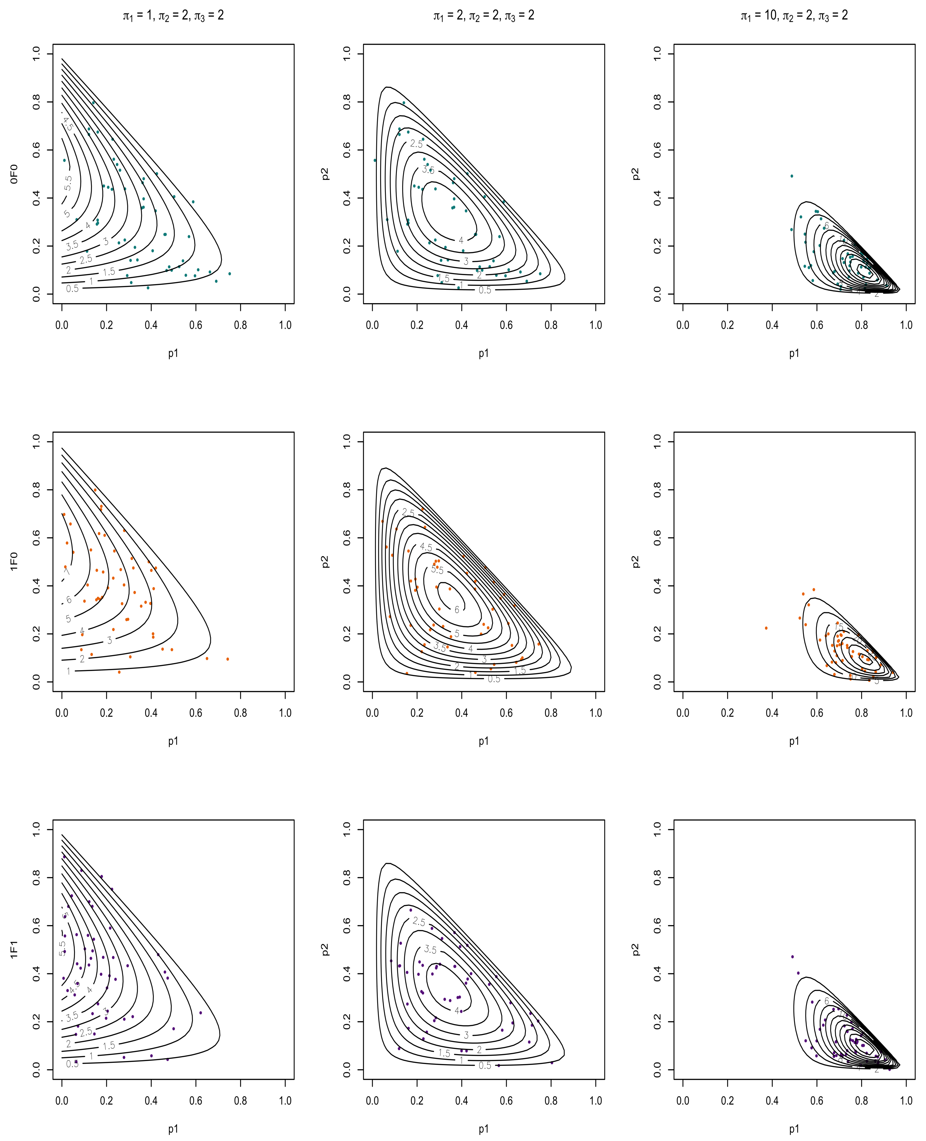
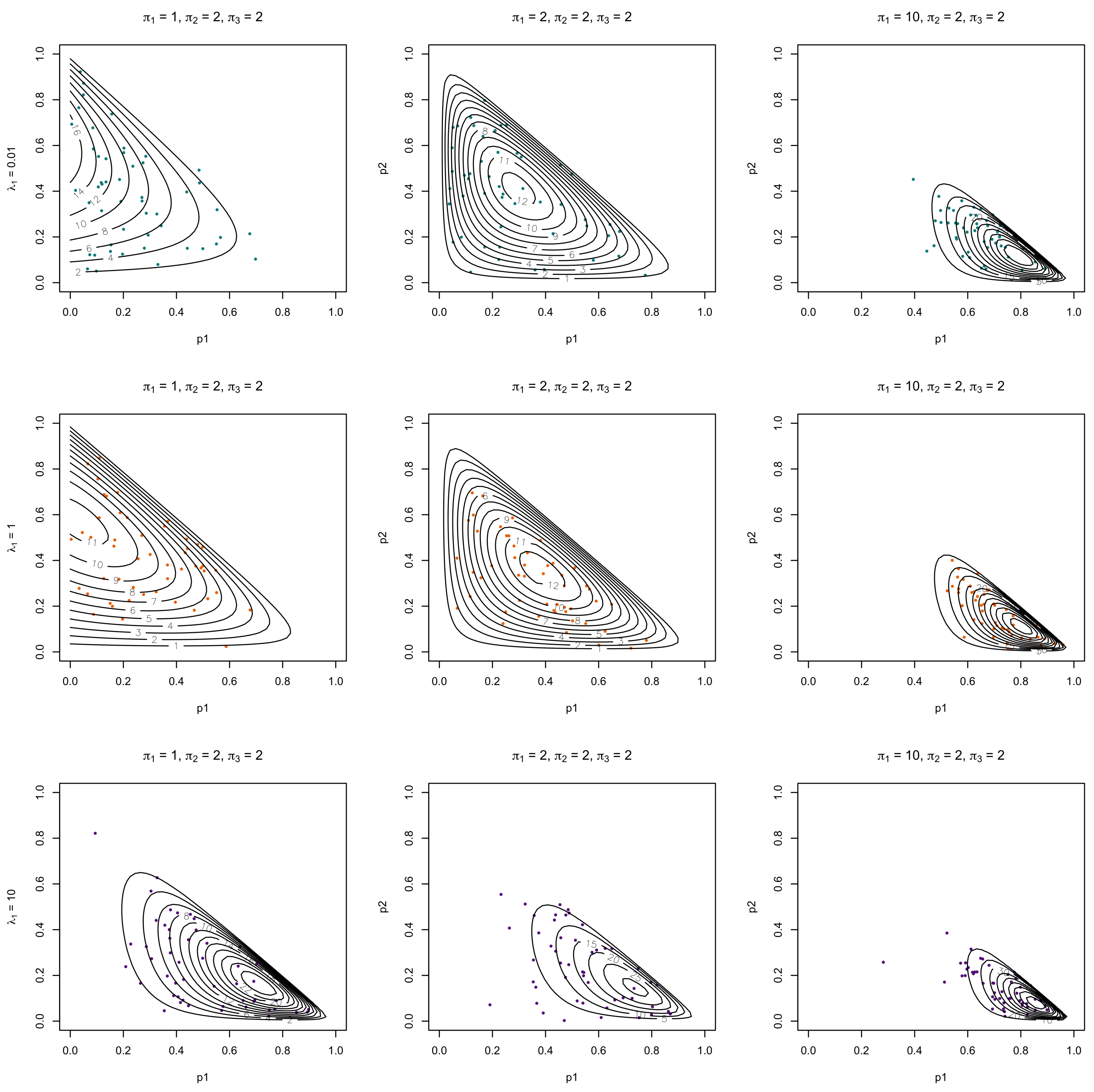
In this paper, three hypergeometric functions are considered (; ), since these are commonly considered functions representing exponential, binomial, and the confluent hypergeometric functions. For illustrative investigation, bivariate observations from the corresponding distributions were simulated using Algorithm 1 and the associated pdfs are overlaid and presented in Figure 1, Figure 2 and Figure 3. The data were simulated from (8) using the following steps of the Acceptance/Rejection method:
| Algorithm 1 Acceptance/Rejection method |
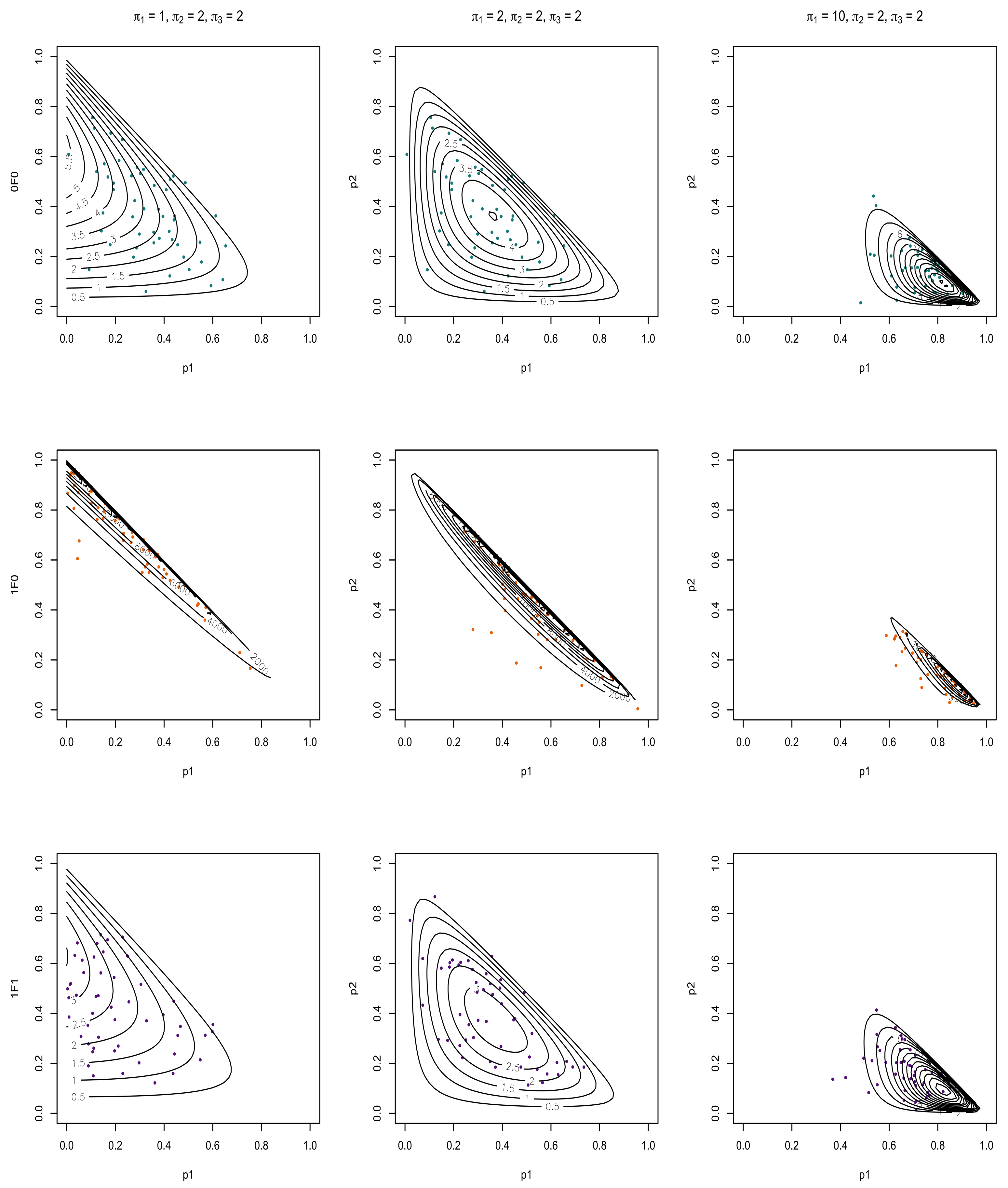
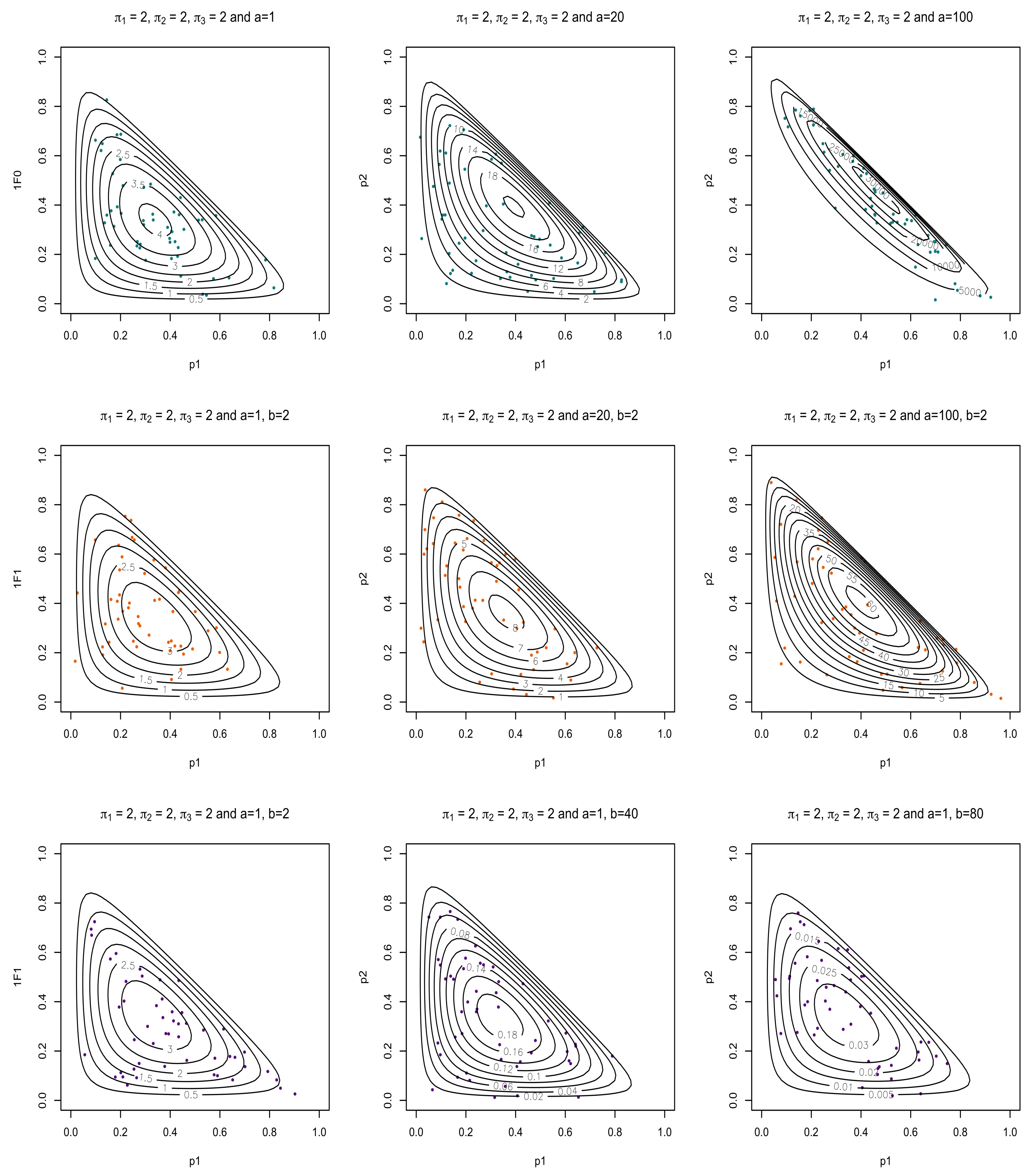
Figure 1 and Figure 2 illustrate the three chosen hypergeometric functions for two choices of and for three different sets of s if with and for , respectively. This firstly illustrates the difference between the different hypergeometric candidates as well as the effect a change in has on these three functions (note that a symmetric observation would be made for ). The difference between Figure 1 and Figure 2 shows the effect that has on these different combinations with Figure 1 having a very small (almost negligible) , while Figure 2 increases the value of . An increase in results in a more highly dense concentration of the pdf for corresponding values of and . This is observed for all three considered hypergeometric candidates, as seen in Figure 1 and Figure 2, also for an increase in . For Figure 3, a single set of s were selected with to showcase the effect that the parameters a and b of the hypergeometric function have on the and functions. As a increases, an increased mass is observed closer to the restriction while an increase in b results in a lower pdf volume.
Next, the posterior distribution is derived, assuming the Dirichlet generator prior (8) together with a multinomial likelihood (1).
Theorem 1.
The complete product moment of the Dirichlet generator posterior (10) is of interest for the power sum (4), thus we are interested in .
Theorem 2.
Suppose that follows a Dirichlet generator posterior distribution with pdf given in (10). Then, the complete product moment is given by
Special cases of the above expression include setting to obtain an expression for the usual product moment of the Dirichlet generator distribution under investigation in this paper.
Proof.
See Appendix A for the proof. □
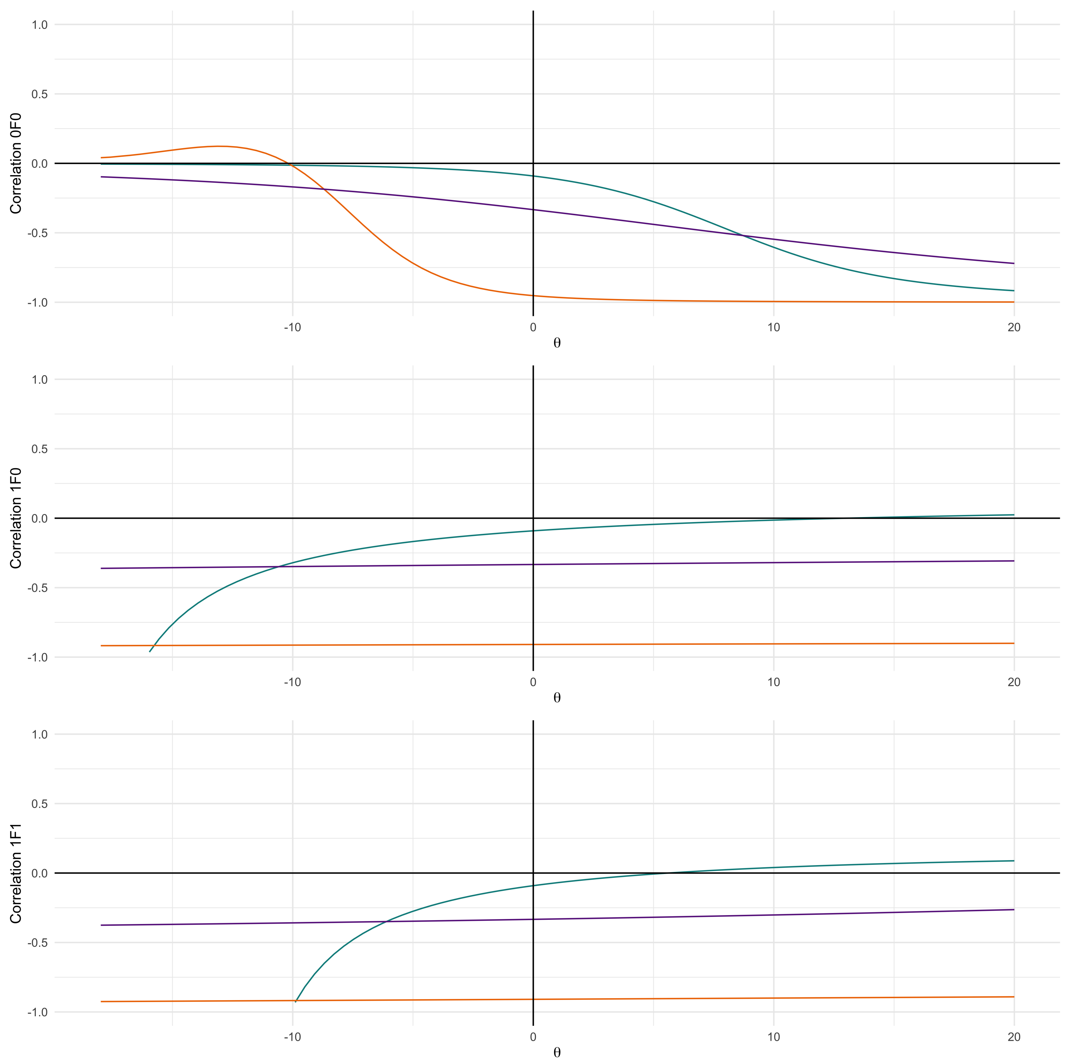
The product moment can then be used to investigate the correlation for the examples as illustrated in this section. Figure 4 displays the correlation for a range of values using (8) and the special cases. It is important to note the positive correlation obtained by the introduction of , which is a major benefit of using these alternative Dirichlet priors.
3.2. Noncentral Dirichlet Prior
In this section, a noncentral Dirichlet distribution will be constructed via the use of Poisson weights. Ref. [16] explored the use of a compounding method as a distributional building tool to obtain bivariate noncentral distributions and showed how this form of the distribution isolated the noncentrality parameter by retaining them in a Poisson probability form and hence introducing mathematical convenience. Ref. [17] extended on this work by introducing new bivariate gamma distributions emanating from a scale mixture of normal class.
Theorem 3.
Suppose is Dirichlet distributed with pdf given by (2). Then, a noncentral Dirichlet distribution can be constructed in the following manner:
where denotes the conditional (central) Dirichlet distribution (see (2)) with parameters , and Λ denotes the vector of noncentral parameters with . After simplification (12) reflects
where denotes the (unconditional) Dirichlet distribution (see (2)) with parameter Π and where .
Remark 1.
The pdf in equation (13) reflects a parametrization of the noncentral Dirichlet distribution of [12] and can be represented via the confluent hypergeometric function of several variables:
where
In particular, when , see that
which illustrates that the model in (12) reduces to the usual (central) Dirichlet model in (2) when the noncentrality parameters are equal to 0. The model in (12) is thus the multivariate analogue of the doubly noncentral beta distribution (see [18]). In the case when is considered in (12), this would represent the multivariate analogue of the singly noncentral beta distribution of [18].
Bivariate observations from the corresponding distributions were simulated using Algorithm 1 and the associated pdfs are overlaid and presented in in Figure 5 for different values of and three combinations of s. These results showcase the effect that has on these three different functions. Figure 5 clearly demonstrates the movement of the centroid of the contour plot.
Next, the posterior distribution is derived, assuming the noncentral Dirichlet prior (12) together with a multinomial likelihood (1).
Theorem 4.
Remark 2.
See that (14) can be represented using the confluent hypergeometric function from Remark 1 as
The complete product moment of the noncentral Dirichlet posterior is of interest for the power sum, thus we are interested in .
Theorem 5.
Suppose that follows a noncentral Dirichlet distribution with pdf given in (14). Then, the complete product moment is given by
Proof.
See Appendix B for the proof. □
4. Entropy Estimates
In this section, the Bayesian estimators (16) and (17) based on the posterior distributions (10) and (14) are derived for the power sum (3).
4.1. Dirichlet Generator Prior
Assuming the Dirichlet generator prior, the posterior distribution is given by (10). Using the complete product moments derived in (11), the Bayesian estimator for the power sum (3) can be derived by setting with and .
Theorem 6.
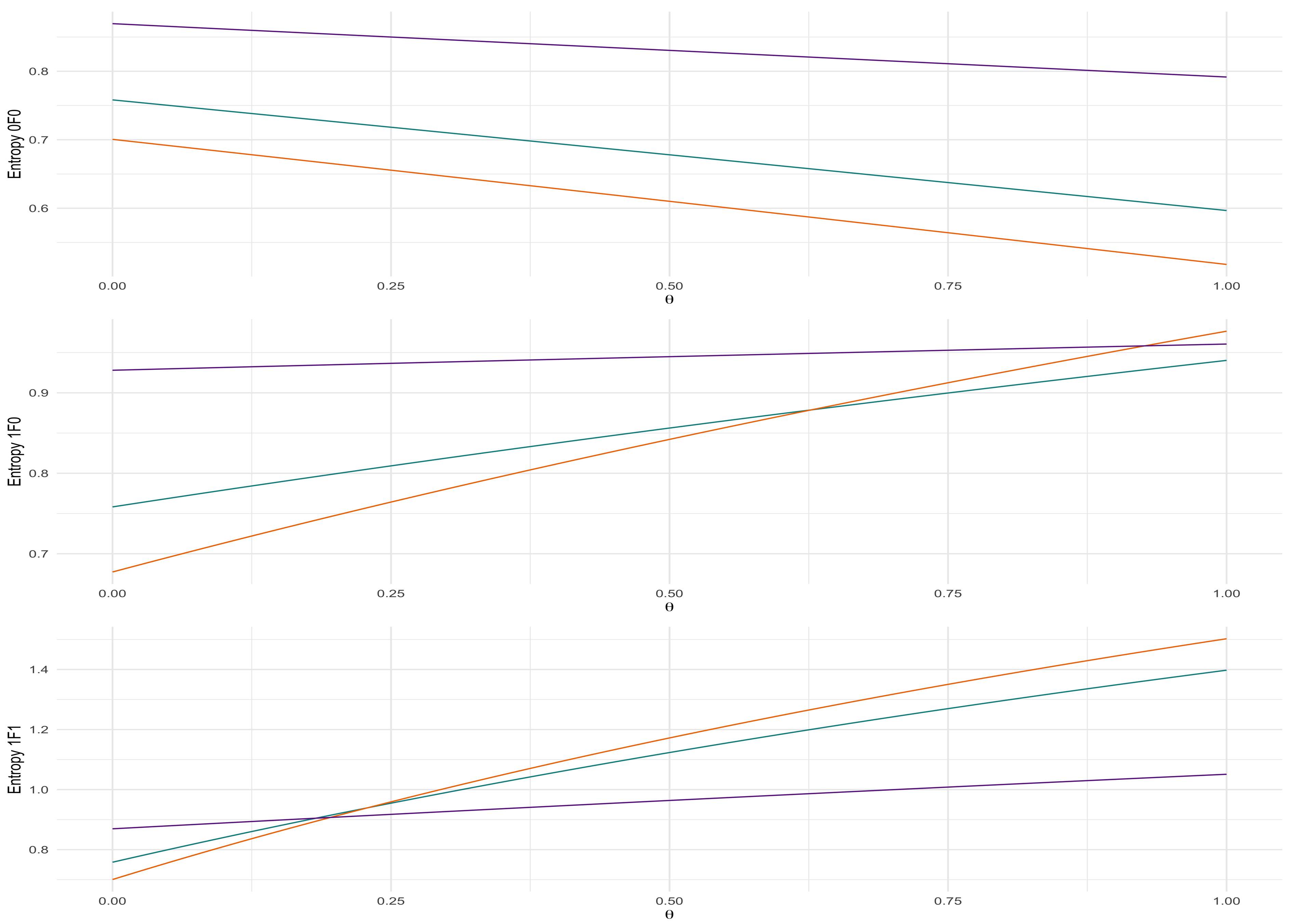
Using the estimated power sum entropy, we can calculate and investigate the behaviour of Tsallis entropy for various parameter scenarios as illustrated in Figure 6 for the bivariate case .
4.2. Noncentral Dirichlet Prior
Assuming the noncentral Dirichlet prior and the posterior distribution is given by (14). Using the complete product moments derived in (15), the Bayesian estimator for the power sum entropy (3) can be derived by setting with and .
Theorem 7.
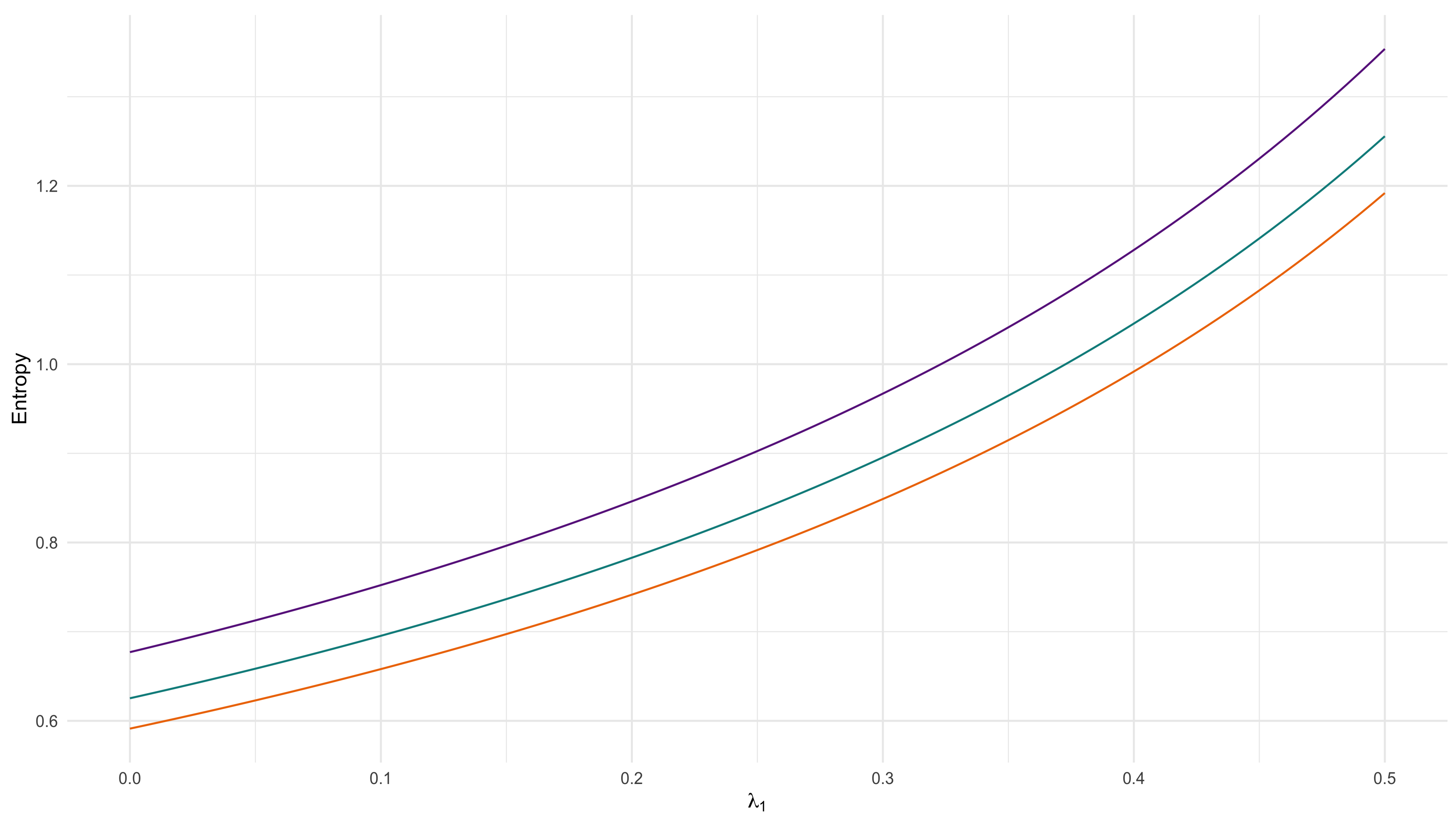
Using the estimated power sum entropy, we can calculate the entropies for different parameters of interests as illustrated in Figure 7 for the bivariate case.
4.3. Numerical Experiments of Entropy
The following steps illustrate the empirical behaviour of the Tsallis entropy under consideration for the alternative priors under consideration (Algorithm 2).
| Algorithm 2 Numerical Experiments of Entropy |
|
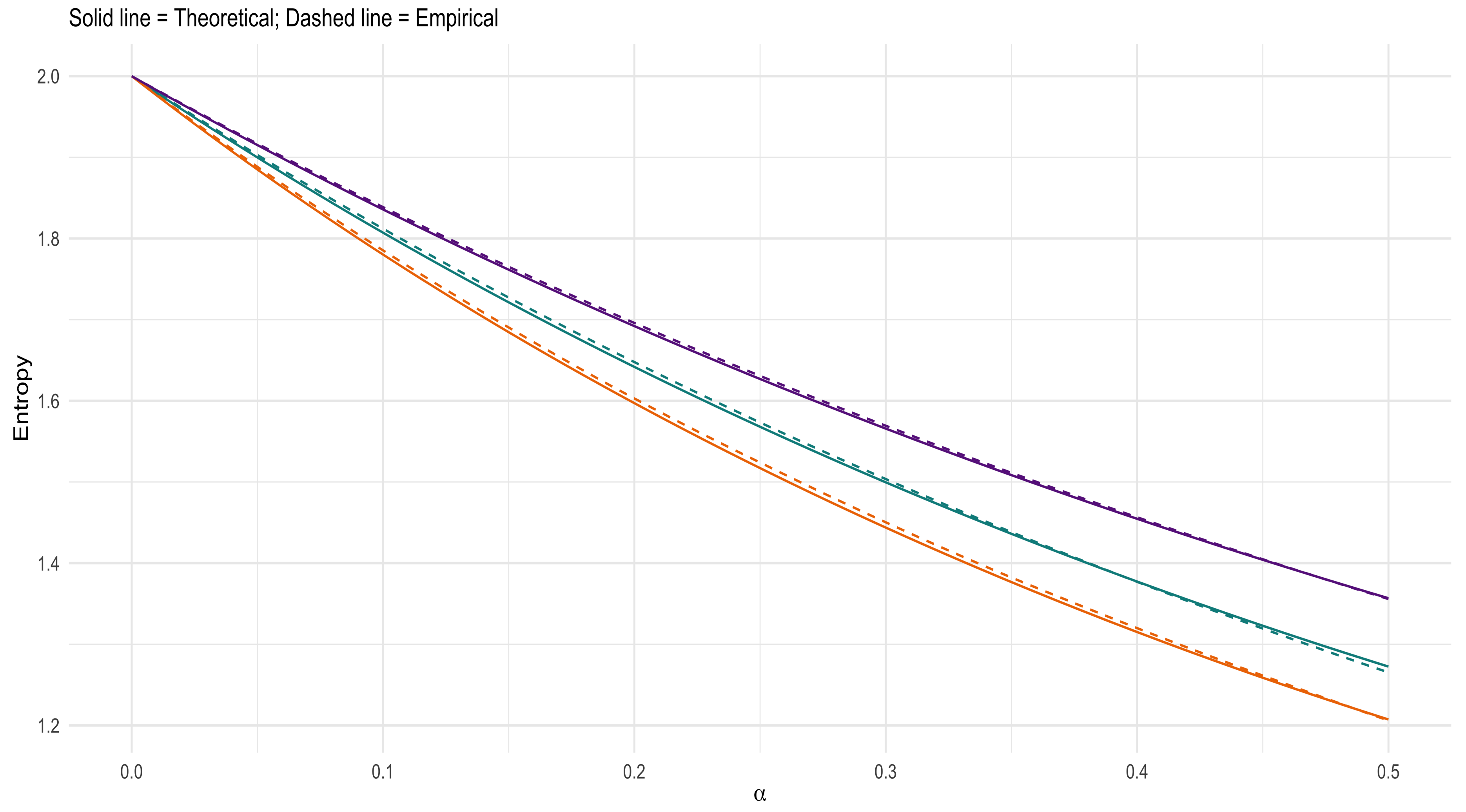
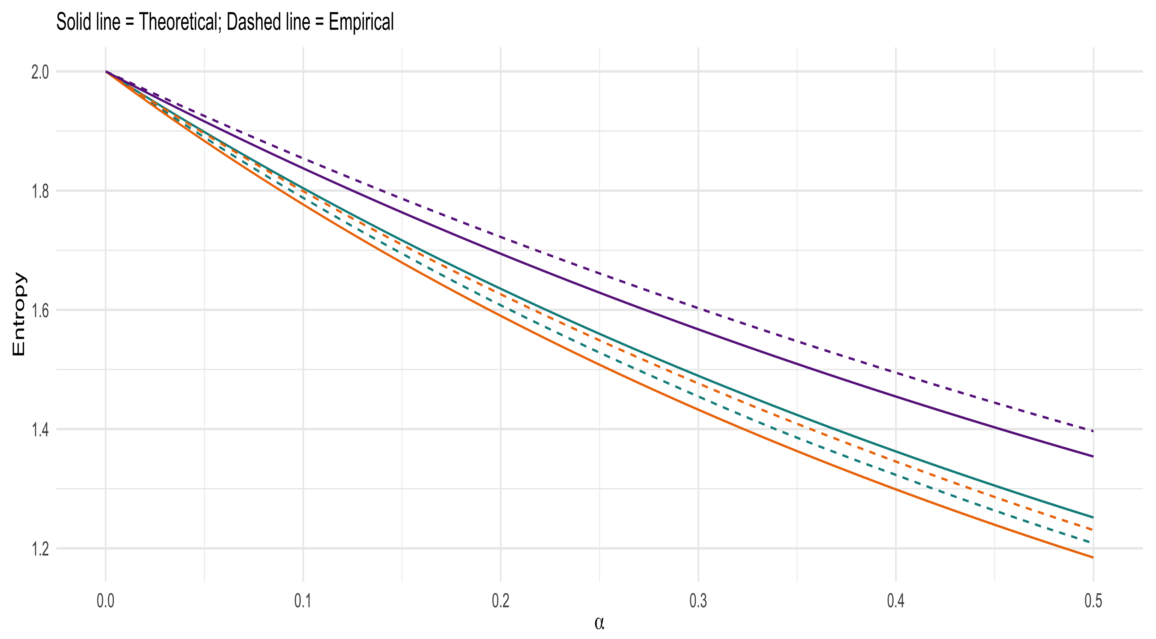
Figure 8 and Figure 9 provides validation of the accuracy of the obtained theoretical expression and contribution for the Dirichlet generator and noncentral Dirichlet cases with , and . From these two figures, it can be seen that the Dirichlet generator prior resulted in empirical results that closely match the theoretical results, while the noncentral Dirichlet shows slight deviations. It is observed that as increases, the Tsallis entropy increases (indicating more uncertainly), while as decreases the Tsallis entropy also decreases (indicating less uncertainty). When considering the location of the density, the changing of leads to densities which tend to the margin of or towards a specific point along the line. This shows that as the concentration of the density moves toward a point along the line, the uncertainty increases and will decrease as the concentration moves towards the small values of .
5. Conclusions
This study focussed on the power sum functional and its estimation as a key tool to model a generalised entropy form, namely Tsallis entropy, via a Bayesian approach. In particular, previous unconsidered Dirichlet priors have been proposed and studied, offering the practitioner more pliable options given experimental data. Specific choices of the proposed Dirichlet family allow for positive correlation in addition to the usual negative correlation characteristic. An example illustrated theoretical results accurately described empirical entropy. Future work could include further investigations into generalised functionals and their modeling in this information-theoretic environment.
Author Contributions
Conceptualization, J.F. and A.B.; methodology, J.F. and A.B.; software, T.B.; validation, T.B., J.F. and A.B.; formal analysis, T.B.; investigation, T.B. and J.F.; writing—original draft preparation, J.F.; writing—review and editing, T.B., J.F. and A.B.; visualization, T.B.; project administration, A.B.; funding acquisition, J.F. and A.B. All authors have read and agreed to the published version of the manuscript.
Funding
This work is based on the research supported in part by the National Research Foundation of South Africa (SARChI Research Chair- UID: 71199; and Grant ref. SRUG190308422768 nr. 120839) as well as the Research Development Programme at the University of Pretoria 296/2021. Opinions expressed and conclusions arrived at are those of the author and are not necessarily to be attributed to the NRF.
Institutional Review Board Statement
Not applicable.
Informed Consent Statement
Not applicable.
Data Availability Statement
Not applicable.
Acknowledgments
The authors would like to thank the anonymous reviewers for their insightful comments which led to the improvement of this paper. The support of the Department of Statistics at the University of Pretoria is acknowledged.
Conflicts of Interest
The authors declare no conflict of interest.
Abbreviations
The following abbreviations are used in this manuscript:
| MLE | Maximum likelihood estimation |
| pmf | Probability mass function |
| Probability density function |
Appendix A. Proof of Complete Product Moments of Dirichlet Generator (11)
Proof.
The definition of the complete product moment of a variate variable with pdf is given by
and since we know that the posterior distribution are given by Dirichlet generator distributions with parameters we can show that:
where C and corresponds to the normalising constants as in (7) and (9), respectively with parameters with parameters and . Since the integral becomes the Dirichlet generator pdf (6) with parameters this will become 1 and the complete product moment will simplify to
□
Appendix B. Proof of Complete Product Moments of Noncentral Dirichlet (15)
Proof.
The definition of the complete product moment of a variate variable with pdf is given by
and since we know that the posterior distribution are given by a noncentral Dirichlet pdf (12) with parameters we can show that
Since the integral becomes the noncentral Dirichlet pdf with parameters this will become 1 and the complete product moment will simplify to
□
References
- Archer, E.; Park, I.M.; Pillow, J. Bayesian entropy estimation for countable discrete distributions. J. Mach. Learn. Res. 2014, 15, 2833–2868. [Google Scholar]
- Ilić, V.; Korbel, J.; Gupta, S.; Scarfone, A.M. An overview of generalized entropic forms. arXiv 2021, arXiv:2102.10071. [Google Scholar]
- Rashad, M.; Iqbal, Z.; Hanif, M. Characterizations and entropy measures of the Libby-Novick generalized beta distribution. Adv. Appl. Stat. 2020, 63, 235–259. [Google Scholar] [CrossRef]
- Jiao, J.; Venkat, K.; Han, Y.; Weissman, T. Maximum likelihood estimation of functionals of discrete distributions. IEEE Trans. Inf. Theory 2017, 63, 6774–6798. [Google Scholar] [CrossRef] [Green Version]
- Contreras Rodríguez, L.; Madarro-Capó, E.J.; Legón-Pérez, C.M.; Rojas, O.; Sosa-Gómez, G. Selecting an Effective Entropy Estimator for Short Sequences of Bits and Bytes with Maximum Entropy. Entropy 2021, 23, 561. [Google Scholar] [CrossRef] [PubMed]
- Wolpert, D.H.; Wolf, D. Estimating functions of probability distributions from a finite set of samples. Phys. Rev. E Stat. Phys. Plasmas Fluids Relat. Interdiscip. Top. 1995, 52, 6841–6854. [Google Scholar] [CrossRef] [PubMed]
- Han, Y.; Jiao, J.; Weissman, T. Does Dirichlet prior smoothing solve the Shannon entropy estimation problem? In Proceedings of the IEEE International Symposium on Information Theory, Hong Kong, China, 14–19 June 2015; pp. 1367–1371. [Google Scholar]
- Little, D.J.; Toomey, J.P.; Kane, D.M. Efficient Bayesian estimation of permutation entropy with Dirichlet priors. arXiv 2021, arXiv:2104.08991. [Google Scholar]
- Zamzami, N.; Bouguila, N. Hybrid generative discriminative approaches based on Multinomial Scaled Dirichlet mixture models. Appl. Intell. 2019, 49, 3783–3800. [Google Scholar] [CrossRef]
- Holste, D.; Grosse, I.; Herzel, H. Bayes’ estimators of generalized entropies. J. Phys. A Math. Gen. 1998, 31, 2551. [Google Scholar] [CrossRef] [Green Version]
- Bodvin, L.J.S.; Bekker, A.; Roux, J.J. Shannon entropy as a measure of certainty in a Bayesian calibration framework with bivariate beta priors: Theory and methods. S. Afr. Stat. J. 2011, 45, 171–204. [Google Scholar]
- Sánchez, L.E.; Nagar, D.; Gupta, A. Properties of noncentral Dirichlet distributions. Comput. Math. Appl. 2006, 52, 1671–1682. [Google Scholar] [CrossRef] [Green Version]
- Kang, M.S.; Kim, K.T. Automatic SAR Image Registration via Tsallis entropy and Iterative Search Process. IEEE Sens. J. 2020, 20, 7711–7720. [Google Scholar] [CrossRef]
- Mathai, A.M.; Haubold, H.J. On generalized entropy measures and pathways. Phys. A Stat. Mech. Appl. 2007, 385, 493–500. [Google Scholar] [CrossRef] [Green Version]
- Gradshteyn, I.S.; Ryzhik, I.M. Table of Integrals, Series, and Products; Academic Press: Cambridge, MA, USA, 2014. [Google Scholar]
- Ferreira, J.T.; Bekker, A.; Arashi, M. Bivariate noncentral distributions: An approach via the compounding method. S. Afr. Stat. J. 2016, 50, 103–122. [Google Scholar]
- Bekker, A.; Ferreira, J.T. Bivariate gamma type distributions for modeling wireless performance metrics. Stat. Optim. Inf. Comput. 2018, 6, 335–353. [Google Scholar] [CrossRef]
- Ongaro, A.; Orsi, C. Some results on non-central beta distributions. Statistica 2015, 75, 85–100. [Google Scholar]
Figure 1.
Dirichlet generator priors (8) for with three different sets of (described above Figure 1), .

Figure 2.
Dirichlet generator priors (8) for with three different sets of , .
Figure 2.
Dirichlet generator priors (8) for with three different sets of , .

Figure 3.
Dirichlet generator priors (8) for with a single set , .
Figure 3.
Dirichlet generator priors (8) for with a single set , .

Figure 4.
Correlation for different candidates. Set 1—blue (); Set 2—orange (); Set 3—purple () with and .
Figure 4.
Correlation for different candidates. Set 1—blue (); Set 2—orange (); Set 3—purple () with and .

Figure 5.
Noncentral Dirichlet Priors (12) for different s with and , .
Figure 5.
Noncentral Dirichlet Priors (12) for different s with and , .

Figure 6.
Dirichlet generator entropy (16)—Varying : Set A—blue () Set B—orange () Set C—purple ().
Figure 6.
Dirichlet generator entropy (16)—Varying : Set A—blue () Set B—orange () Set C—purple ().

Figure 7.
Noncentral Dirichlet Entropy—Varying : Set A—blue () Set B—orange () Set C—purple ().

Figure 8.
Dirichlet generator —empirical vs calculated Tsallis entropy: for and Set A—blue () Set B—orange () Set C—purple ().
Figure 8.
Dirichlet generator —empirical vs calculated Tsallis entropy: for and Set A—blue () Set B—orange () Set C—purple ().

Figure 9.
Noncentral Dirichlet—empirical vs calculated Tsallis entropy: for and with Set A—blue () Set B—orange () Set C—purple ().
Figure 9.
Noncentral Dirichlet—empirical vs calculated Tsallis entropy: for and with Set A—blue () Set B—orange () Set C—purple ().

Publisher’s Note: MDPI stays neutral with regard to jurisdictional claims in published maps and institutional affiliations. |
© 2021 by the authors. Licensee MDPI, Basel, Switzerland. This article is an open access article distributed under the terms and conditions of the Creative Commons Attribution (CC BY) license (https://creativecommons.org/licenses/by/4.0/).
Share and Cite
MDPI and ACS Style
Botha, T.; Ferreira, J.; Bekker, A. Alternative Dirichlet Priors for Estimating Entropy via a Power Sum Functional. Mathematics 2021, 9, 1493. https://0-doi-org.brum.beds.ac.uk/10.3390/math9131493
AMA Style
Botha T, Ferreira J, Bekker A. Alternative Dirichlet Priors for Estimating Entropy via a Power Sum Functional. Mathematics. 2021; 9(13):1493. https://0-doi-org.brum.beds.ac.uk/10.3390/math9131493
Chicago/Turabian StyleBotha, Tanita, Johannes Ferreira, and Andriette Bekker. 2021. "Alternative Dirichlet Priors for Estimating Entropy via a Power Sum Functional" Mathematics 9, no. 13: 1493. https://0-doi-org.brum.beds.ac.uk/10.3390/math9131493
Note that from the first issue of 2016, this journal uses article numbers instead of page numbers. See further details here.