On the Convergence of a New Family of Multi-Point Ehrlich-Type Iterative Methods for Polynomial Zeros

Abstract

In this paper, we construct and study a new family of multi-point Ehrlich-type iterative methods for approximating all the zeros of a uni-variate polynomial simultaneously. The first member of this family is the two-point Ehrlich-type iterative method introduced and studied by Trićković and Petković in 1999. The main purpose of the paper is to provide local and semilocal convergence analysis of the multi-point Ehrlich-type methods. Our local convergence theorem is obtained by an approach that was introduced by the authors in 2020. Two numerical examples are presented to show the applicability of our semilocal convergence theorem.

1. Introduction

This work deals with multi-point iterative methods for approximating all the zeros of a polynomial simultaneously. Let us recall that an iterative method for solving a nonlinear equation is called a multi-point method if it can be defined by an iteration of the form

$$x^{(k+1)}=\phi (x^{\left(k\right)},x^{(k-1)},\dots ,x^{(k-N)}),k=0,1,2,\dots ,$$

where N is a fixed natural number, and $x^{\left(0\right)},x^{(-1)},\dots ,x^{(-N)}$ are $N+1$ initial approximations. In the literature, there are multi-point iterative methods for finding a single zero of a nonlinear equation (see, e.g., [1,2,3,4,5,6,7]). This study is devoted to the multi-point iterative methods for approximating all the zeros of a polynomial simultaneously (see, e.g., [8,9,10,11]).

Let us recall the two most popular iterative methods for simultaneous computation of all the zeros of a polynomial f of degree $n\ge 2$. These are Weierstrass’ method [12] and Ehrlich’s method [13].

Weierstrass’ method is defined by the following iteration:

$$x^{(k+1)}=x^{\left(k\right)}-W_f\left(x^{\left(k\right)}\right),k=0,1,2,\dots ,$$

(1)

where the function $W_f:\mathcal{D}\subset {\mathbb{K}}^n\to {\mathbb{K}}^n$ is defined by $W_f\left(x\right)=\left(W_1\left(x\right),\dots ,W_n\left(x\right)\right)$ with

$$W_i\left(x\right)=\frac{f\left(x_i\right)}{{\displaystyle a_0\prod _{j\ne i}(x_i-x_j)}}(i=1,\dots ,n),$$

(2)

where $a_0\in \mathbb{K}$ is the leading coefficient of f and $\mathcal{D}$ denotes the set of all vectors in ${\mathbb{K}}^n$ with pairwise distinct components. Weierstrass’ method (1) has second order of convergence (provided that f has only simple zeros).

Ehrlich’s method is defined by the following fixed point iteration:

$$x^{(k+1)}=T\left(x^{\left(k\right)}\right),k=0,1,2,\dots ,$$

(3)

where the iteration function $T:{\mathbb{K}}^n\to {\mathbb{K}}^n$ is defined by $T\left(x\right)=(T_1\left(x\right),\dots ,T_n\left(x\right))$ with

$$T_i\left(x\right)=x_i-\frac{f\left(x_i\right)}{{\displaystyle f^{\prime }\left(x_i\right)-f\left(x_i\right)\sum _{j\ne i}\frac{1}{x_i-x_j}}}(i=1,\dots ,n).$$

(4)

Ehrlich’s method has third order convergence. In 1973, this method was rediscovered by Aberth [14]. In 1970, Börsch-Supan [15] constructed another third-order method for simultaneous computing all the zeros of a polynomial. However in 1982, Werner [16] proved that both Ehrlich’s and Börsch-Supan’s methods are identical.

In 1999, Trićković and Petković [9] constructed and studied a two-point version of Ehrlich’s method. They proved that the two-point Ehrlich-type method has the order of convergence $r=1+\sqrt{2}$.

In the present paper, we introduce an infinite sequence of multi-point Ehrlich-type iterative methods. We note that the first member of this family of iterative methods is the two-point Ehrlich-type method constructed in [9]. The main purpose of this paper is to provide a local and semilocal convergence analysis of the multi-point Ehrlich-type methods.

Our local convergence result (Theorem 2) contains the following information: convergence domain; a priori and a posteriori error estimates; convergence order of every method of the family. For instance, we prove that for a given natural number N, the order of convergence of the Nth multi-point Ehrlich-type method is $r=r\left(N\right)$, where r is the unique positive solution of the equation

$$1+2(t+\dots +t^N)=t^{N+1}.$$

(5)

It follows from this result that the first iterative method $(N=1)$ has the order of convergence $r\left(1\right)=1+\sqrt{2}$ which coincides with the above mentioned result of Trićković and Petković. We note that each method of the new family has super-quadratic convergence of order $r\in [1+\sqrt{2},3)$. The semilocal convergence result (Theorem 4) states a computer-verifiable initial condition that guarantees fast convergence of the corresponding method of the family.

The paper is structured as follows: In Section 2, we introduce the new family of multi-point iterative methods. Section 3 contains some auxiliary results that underlie the proofs of the main results. In Section 3, we present a local convergence result (Theorem 2) for the iterative methods of the new family. This result contains initial conditions as well as a priori and a posteriori error estimates. In Section 5, we provide a semilocal convergence result (Theorem 4) with computer verifiable initial conditions. Section 6 provides two numerical examples to show the applicability of our semilocal convergence theorem and the convergence behavior of the proposed multi-point iterative methods. The paper ends with a conclusion section.

2. A New Family of Multi-Point Ehrlich-Type Iterative Methods

Throughout the paper $(\mathbb{K},|·\left|\right)$ stands for a valued field with a nontrivial absolute value $|·|$ and $\mathbb{K}\left[z\right]$ denotes the ring of uni-variate polynomials over $\mathbb{K}$. The vector space ${\mathbb{K}}^n$ is equipped with the product topology.

For a given vector $u\in {\mathbb{K}}^n$, $u_i$ always denotes the ith component of u. For example, if F is a map with values in ${\mathbb{K}}^n$, then $F_i\left(x\right)$ denotes the ith component of the vector $F\left(x\right)\in {\mathbb{K}}^n$. Let us define a binary relation $\#$ on ${\mathbb{K}}^n$ as follows [17]

$$u\#v\iff u_i\ne v_j\mathrm{for}\mathrm{all}i,j\in I_n\mathrm{with}i\ne j.$$

Here and throughout the paper, $I_n$ is defined by

$$I_n=\{1,2,\dots ,n\}.$$

Suppose $f\in \mathbb{K}\left[z\right]$ is a polynomial of degree $n\ge 2$. A vector $\xi \in {\mathbb{K}}^n$ is called a root vector of the polynomial f if

$$f\left(z\right)=a_0\prod _{i=1}^n(z-{\xi }_i)\mathrm{for}\mathrm{all}z\in \mathbb{K},$$

where $a_0\in \mathbb{K}$. It is obvious that f possesses a root vector in ${\mathbb{K}}^n$ if and only if it splits over $\mathbb{K}$.

In the following definition, we introduce a real-value function of two vector variables that plays an essential role in the present study.

Definition 1.

Suppose $f\in \mathbb{K}\left[z\right]$ is a polynomial of degree $n\ge 2$. We define an iteration function $\Phi :D_{\Phi }\subset {\mathbb{K}}^n\times {\mathbb{K}}^n\to {\mathbb{K}}^n$ of two vector variables as follows:

$${\Phi }_i(x,y)=x_i-\frac{f\left(x_i\right)}{{\displaystyle f^{\prime }\left(x_i\right)-f\left(x_i\right)\sum _{j\ne i}\frac{1}{x_i-y_j}}}(i=1,\dots ,n),$$

(6)

where $D_{\Phi }$ is defined by

$$D_{\Phi }=\left\{{\displaystyle (x,y)\in {\mathbb{K}}^n\times {\mathbb{K}}^n:x\#y,f^{\prime }\left(x_i\right)-f\left(x_i\right)\sum _{j\ne i}\frac{1}{x_i-y_j}\ne 0\mathrm{for}i\in I_n}\right\}.$$

(7)

Now the two-point Ehrlich-type root-finding method introduced by Trićković and Petković [9] can be defined by the following iteration

$$x^{(k+1)}=\Phi (x^{\left(k\right)},x^{(k-1)}),k=0,1,\dots$$

(8)

with initial approximations $x^{\left(0\right)},x^{(-1)}\in {\mathbb{K}}^n$.

Theorem 1

(Petković and Trićkovic [9]). The convergence order of the two-point Ehrlich-type method (8) is $r=1+\sqrt{2}\approx 2.414$.

Based on the function $\Phi$, we define a sequence ${\left({\Phi }^{\left(N\right)}\right)}_{N=1}^{\infty }$ of vector-valued functions such that the Nth function ${\Phi }^{\left(N\right)}$ is a function of $N+1$ vector variables.

Definition 2.

We define a sequence ${\left({\Phi }^{\left(N\right)}\right)}_{N=0}^{\infty }$ of iteration functions

$${\Phi }^{\left(N\right)}:D_N\subset \underset{N+1}{\underbrace{{\mathbb{K}}^n\times \dots \times {\mathbb{K}}^n}}\to {\mathbb{K}}^n$$

recursively by setting ${\Phi }^{\left(0\right)}\left(x\right)=x$ and

$${\Phi }^{\left(N\right)}(x,y,\dots ,z)=\Phi (x,{\Phi }^{(N-1)}(y,\dots ,z)).$$

(9)

The sequence ${\left(D_N\right)}_{N=0}^{\infty }$ of domains is defined also recursively by setting $D_0={\mathbb{K}}^n$ and

$$\begin{array}{cc}\hfill D_N=& \left\{(x,y,\dots ,z)\in \underset{N+1}{\underbrace{{\mathbb{K}}^n\times \dots \times {\mathbb{K}}^n}}:(y,\dots ,z)\in D_{N-1},x\#{\Phi }^{(N-1)}(y,\dots ,z)\right.\hfill \\ \hfill & \left.{\displaystyle \mathrm{and}{f}^{\prime }\left(x_i\right)-f\left(x_i\right)\sum _{j\ne i}\frac{1}{x_i-{\Phi }_j^{(N-1)}(y,\dots ,z)}\ne 0\mathrm{for}i\in I_n}\right\}.\hfill \end{array}$$

(10)

Clearly, the iteration function ${\Phi }^{\left(1\right)}$ coincides with the function $\Phi$.

Definition 3.

Let N be a given natural number, and $x^{\left(0\right)},x^{(-1)},\dots ,x^{(-N)}\in {\mathbb{K}}^n$ be $N+1$ initial approximations. We define the Nth iterative method of an infinite sequence of multi-point Ehrlich-type methods by the following iteration

$$x^{(k+1)}={\Phi }^{\left(N\right)}(x^{\left(k\right)},x^{(k-1)},\dots ,x^{(k-N)}),k=0,1,\dots .$$

(11)

Note that in the case $N=1$, the iterative method (11) coincides with the two-point Ehrlich-type method (8).

In Section 4, we present a local convergence theorem (Theorem 2) for the methods (11) with initial conditions that guarantee the convergence to a root vector of f. In the case $N=1$, this result extends Theorem 1 in several directions.

In Section 5, we present a semilocal convergence theorem (Theorem 4) for the family (11), which is of practical importance.

3. Preliminaries

In this section, we present two basic properties of the iteration function $\Phi$ defined in Definition 1, which play an important role in obtaining the main result in Section 4.

In what follows, we assume that ${\mathbb{K}}^n$ is endowed with the norm ${\parallel ·\parallel }_{\infty }$ defined by

$${\parallel u\parallel }_{\infty }=max\left\{\right|u_1|,\dots ,|u_n\left|\right\}$$

and with the cone norm $\parallel ·\parallel :{\mathbb{K}}^n\to {\mathbb{R}}^n$ defined by

$$\parallel u\parallel =\left(\right|u_1|,\dots ,|u_n\left|\right),$$

assuming that ${\mathbb{R}}^n$ is endowed with the component-wise ordering ⪯ defined by

$$u⪯v\iff u_i\le v_i\mathrm{for}\mathrm{all}i\in I_n.$$

Furthermore, for two vectors $u\in {\mathbb{K}}^n$ and $v\in {\mathbb{R}}^n$, we denote by $u/v$ the vector

$$\frac{u}{v}=\left(\frac{|u_1|}{v_1},\cdots ,\frac{|u_n|}{v_n}\right).$$

We define a function $d:{\mathbb{K}}^n\to {\mathbb{R}}^n$ by $d\left(u\right)=(d_1\left(u\right),\dots ,d_n\left(u\right))$ with

$$d_i\left(u\right)=\underset{j\ne i}{min}|u_i-u_j|(i=1,\dots ,n).$$

Lemma 1

([11]). Suppose $x,y,\xi \in {\mathbb{K}}^n$ and ξ is a vector with pairwise distinct components.

$$|x_i-y_j|\ge (1-E\left(x\right)-E\left(y\right))|{\xi }_i-{\xi }_j|\mathrm{for}\mathrm{all}i,j\in I_n,$$

(12)

where the function $E:{\mathbb{K}}^n\to {\mathbb{R}}_{+}$ is defined by

$$E\left(x\right)={∥\frac{x-\xi }{d\left(\xi \right)}∥}_{\infty }.$$

(13)

Lemma 2.

Suppose $f\in \mathbb{K}\left[z\right]$ is a polynomial of degree $n\ge 2$, which splits over $\mathbb{K}$, and $\xi \in {\mathbb{K}}^n$ is a root vector of f. Let $x,y\in {\mathbb{K}}^n$ be two vectors such that $x\#y$. If $f\left(x_i\right)\ne 0$ for some $i\in I_n$, then

$$\frac{f^{\prime }\left(x_i\right)}{f\left(x_i\right)}-\sum _{j\ne i}{\displaystyle \frac{1}{x_i-y_j}}=\frac{1-{\tau }_i}{x_i-{\xi }_i},$$

(14)

where ${\tau }_i\in \mathbb{K}$ is defined by

$${\tau }_i=(x_i-{\xi }_i)\sum _{j\ne i}{\displaystyle \frac{y_j-{\xi }_j}{(x_i-{\xi }_j)(x_i-y_j)}}.$$

(15)

Proof. 

Since $\xi$ is a root vector of f, we obtain

$${\displaystyle \frac{f^{\prime }\left(x_i\right)}{f\left(x_i\right)}-\sum _{j\ne i}{\displaystyle \frac{1}{x_i-y_j}}=\sum _{j=1}^n\frac{1}{x_i-{\xi }_i}-\sum _{j\ne i}\frac{1}{x_i-y_j}=\frac{1}{x_i-{\xi }_i}+\sum _{j\ne i}\left(\frac{1}{x_i-{\xi }_j}+\frac{1}{x_i-y_j}\right)}$$

$$=\frac{1}{x_i-{\xi }_i}-\sum _{j\ne i}\frac{y_j-{\xi }_j}{(x_i-{\xi }_j)(x_i-y_j)}=\frac{1-{\tau }_i}{x_i-{\xi }_i},$$

which proves (14). □

Define the function $\sigma :\mathcal{D}\subset {\mathbb{K}}^n\times {\mathbb{K}}^n\to {\mathbb{R}}_{+}$ by

$$\sigma (x,y)=\frac{(n-1)E\left(x\right)E\left(y\right)}{(1-E(x\left)\right)(1-E(x)-E(y\left)\right)-(n-1)E\left(x\right)E\left(y\right)}$$

(16)

with domain

$$\mathcal{D}=\left\{(x,y)\in {\mathbb{K}}^n\times {\mathbb{K}}^n:(1-E\left(x\right))(1-E\left(x\right)-E\left(y\right))>(n-1)E\left(x\right)E\left(y\right)\mathrm{and}E\left(x\right)+E\left(y\right)<1\right\},$$

(17)

where $E:{\mathbb{K}}^n\to {\mathbb{R}}_{+}$ is defined by (13).

Lemma 3.

Let $f\in \mathbb{K}\left[z\right]$ be a polynomial of degree $n\ge 2$ with n simple zeros in $\mathbb{K}$, and let $\xi \in {\mathbb{K}}^n$ be a root vector of f. Suppose $x,y\in {\mathbb{K}}^n$ are two vectors such that $(x,y)\in \mathcal{D}$. Then:

(i)

$(x,y)\in D_{\Phi }$;

(ii)

$\parallel \Phi (x,y)-\xi \parallel ⪯\sigma (x,y)\parallel x-\xi \parallel$;

(iii)

$E(\Phi (x,y\left)\right)\le \sigma (x,y)E\left(x\right)$,

where the functions Φ, E and σ are defined by (6), (13) and (16), respectively.

Proof. (i) According to (17), we have $E\left(x\right)+E\left(y\right)<1$. Then it follows from Lemma 1 that

$$|x_i-y_j|\ge (1-E\left(x\right))d_j\left(\xi \right)>0$$

(18)

for every $j\ne i$. This yields $x\#y$. In view of (7), it remains to prove that

$$f^{\prime }\left(x_i\right)-f\left(x_i\right)\sum _{j\ne i}{\displaystyle \frac{1}{x_i-y_j}}\ne 0$$

(19)

for $i\in I_n$. Let $i\in I_n$ be fixed. We shall consider only the non-trivial case $f\left(x_i\right)\ne 0$. In this case, (19) is equivalent to

$$\frac{f^{\prime }\left(x_i\right)}{f\left(x_i\right)}-\sum _{j\ne i}{\displaystyle \frac{1}{x_i-y_j}}\ne 0.$$

(20)

On the other hand, it follows from Lemma 2 that (20) is equivalent to ${\tau }_i\ne 1$, where ${\tau }_i$ is defined by (15). By Lemma 1 with $y=\xi$, we obtain

$$|x_i-{\xi }_j|\ge (1-E\left(x\right))d_i\left(\xi \right)>0$$

(21)

for every $j\ne i$. From (15), (18) and (21), we obtain

$$\begin{array}{ccc}\hfill & |{\tau }_i|& \le |x_i-{\xi }_i|\sum _{j\ne i}\frac{|y_j-{\xi }_j|}{|x_i-{\xi }_j\left|\right|x_i-y_j|}\hfill \\ \hfill & & \le \frac{1}{(1-E(x\left)\right)(1-E(x)-E(y\left)\right)}\frac{|x_i-{\xi }_i|}{d_i\left(\xi \right)}\sum _{j\ne i}\frac{|y_j-{\xi }_j|}{d_j\left(\xi \right)}\hfill \\ \hfill & & \le \frac{(n-1)E\left(x\right)E\left(y\right)}{(1-E(x\left)\right)(1-E(x)-E(y\left)\right)}<1.\hfill \end{array}$$

(22)

This implies that ${\tau }_i\ne 1$ which proves the first claim.

(ii) The second claim is equivalent to

$$|{\Phi }_i(x,y)-{\xi }_i|\le \sigma (x,y)|x_i-{\xi }_i|$$

(23)

for all $i\in I_n$. If $x_i={\xi }_i$, then (23) holds trivially. Let $x_i\ne {\xi }_i$. Then, it follows from (21) that $f\left(x_i\right)\ne 0$. It follows from (6), (20) and (14) that

$$\begin{array}{ccc}\hfill & {\Phi }_i(x,y)-{\xi }_i& =x_i-{\xi }_i-{\left(\frac{f^{\prime }\left(x_i\right)}{f\left(x_i\right)}-\sum _{j\ne i}\frac{1}{x_i-y_j}\right)}^{-1}\hfill \\ \hfill & & =x_i-{\xi }_i-\frac{x_i-{\xi }_i}{1-{\tau }_i}=-\frac{{\tau }_i}{1-{\tau }_i}(x_i-{\xi }_i).\hfill \end{array}$$

(24)

By (24) and the estimate (22), we obtain

$$\begin{array}{ccc}& |{\Phi }_i(x,y)-{\xi }_i|& =\frac{|{\tau }_i|}{|1-{\tau }_i|}|x_i-{\xi }_i|\le \frac{|{\tau }_i|}{1-|{\tau }_i|}|x_i-{\xi }_i|\hfill \\ & & \le \frac{(n-1)E\left(x\right)E\left(y\right)}{(1-E(x\left)\right)(1-E(x)-E(y\left)\right)-(n-1)E\left(x\right)E\left(y\right)}|x_i-{\xi }_i|\hfill \\ & & \hfill \\ & & =\sigma (x,y)|x_i-{\xi }_i|.\hfill \end{array}$$

Therefore, (23) holds, which proves the second claim.

(iii) By dividing both sides of the last inequality by $d_i\left(\xi \right)$ and taking the max-norm, we obtain the third claim. □

Lemma 4.

Let $f\in \mathbb{K}\left[z\right]$ be a polynomial of degree $n\ge 2$ with n simple zeros in $\mathbb{K}$, and let $\xi \in {\mathbb{K}}^n$ be a root vector of f. Suppose $x,y\in {\mathbb{K}}^n$ are two vectors satisfying

$$max\left\{E\left(x\right),E\left(y\right)\right\}\le R=\frac{2}{3+\sqrt{8n-7}},$$

(25)

where the function $E:{\mathbb{K}}^n\to {\mathbb{R}}_{+}$ is defined by (13). Then:

(i)

$(x,y)\in \mathcal{D}$;

(ii)

${\displaystyle \sigma (x,y)\le \frac{E\left(x\right)E\left(y\right)}{R^2}}$;

(iii)

${\displaystyle E(\Phi (x,y))\le \frac{E{\left(x\right)}^{2}E\left(y\right)}{R^2}}$.

Proof. 

It follows from (25) that $E\left(x\right)+E\left(y\right)\le 2R<1$ and

$$(1-E\left(x\right))(1-E\left(x\right)-E\left(y\right))-(n-1)E\left(x\right)E\left(y\right)\ge (1-R)(1-2R)-(n-1)R^2>0.$$

(26)

Hence, it follows from (17) that $(x,y)\in \mathcal{D}$ which proves the claim (i). It is easy to show that R is the unique positive zero of the function $\varphi$, defined by

$$\varphi \left(t\right)=\frac{(n-1)t^2}{(1-t)(1-2t)-(n-1)t^2}.$$

(27)

Then, from (16) and (26), we obtain

$$\begin{array}{ccc}& \sigma (x,y)& \le \frac{(n-1)E\left(x\right)E\left(y\right)}{(1-R)(1-2R)-(n-1)R^2}\hfill \\ & & =\frac{(n-1)R^2}{(1-R)(1-2R)-(n-1)R^2}\frac{E\left(x\right)E\left(y\right)}{R^2}\hfill \\ & & =\varphi \left(R\right)\frac{E\left(x\right)E\left(y\right)}{R^2}=\frac{E\left(x\right)E\left(y\right)}{R^2},\hfill \end{array}$$

(28)

which proves (ii). The claim (iii) follows from Lemma 3 (iii) and claim (ii). □

4. Local Convergence Analysis

In this section, we present a local convergence theorem for the multi-point iterative methods (11). More precisely, we study the local convergence of the multi-point Ehrlich-type methods (11) with respect to the function of the initial conditions $E:{\mathbb{K}}^n\to {\mathbb{R}}_{+}$ defined by (13), where $\xi \in {\mathbb{K}}^n$ is a root vector of a polynomial $f\in \mathbb{K}\left[z\right]$.

Definition 4.

We define a sequence ${\left({\sigma }_N\right)}_{N=1}^{\infty }$ of functions ${\sigma }_N:{\mathcal{D}}_N\subset {\underbrace{{\mathbb{K}}^n\times \dots \times {\mathbb{K}}^n}}_{N+1}\to \mathbb{R}$ by

$${\sigma }_N(x,y,\dots ,z)=\sigma (x,{\Phi }^{(N-1)}(y,\dots ,z)),$$

(29)

where σ is defined by (16). The domain ${\mathcal{D}}_N$ is defined by

$$\begin{array}{cc}\hfill {\mathcal{D}}_N=& \{(x,y,\dots ,z):x\in {\mathbb{K}}^n,(y,\dots ,z)\in D_{N-1},\hfill \\ & (1-E\left(x\right))(1-E\left(x\right)-E\left({\Phi }^{(N-1)}(y,\dots ,z)\right))>(n-1)E\left(x\right)E\left({\Phi }^{(N-1)}(y,\dots ,z)\right),\hfill \\ & E\left(x\right)+E\left({\Phi }^{(N-1)}(y,\dots ,z)\right)<1\},\hfill \end{array}$$

and $D_N$ is defined by (10).

Lemma 5.

Let $f\in \mathbb{K}\left[z\right]$ be a polynomial of degree $n\ge 2$ with n simple zeros in $\mathbb{K}$ and $\xi \in {\mathbb{K}}^n$ be a root vector of f. Assume $N\ge 1$ and $(x,y,\dots ,z)\in {\mathcal{D}}_N$. Then:

(i)

$(x,y,\dots ,z)\in D_N$;

(ii)

$\parallel {\Phi }^{\left(N\right)}(x,y,\dots ,z)-\xi \parallel ⪯{\sigma }_N(x,y,\dots ,z)\parallel x-\xi \parallel$;

(iii)

$E\left({\Phi }^{\left(N\right)}(x,y,\dots ,z)\right)\le {\sigma }_N(x,y,\dots ,z)E\left(x\right)$,

where ${\Phi }^{\left(N\right)}$ and ${\sigma }_N$ are defined by (9) and (29), respectively.

Proof. 

Applying Lemma 1 with $y={\Phi }^{(N-1)}(y,\dots ,z)$, we obtain (i). It follows from Definition 2, Lemma 3 (ii) and Definition 4 that

$$\begin{array}{c}\hfill \parallel {\Phi }^{\left(N\right)}(x,y,\dots ,z)-\xi \parallel =\parallel \Phi (x,{\Phi }^{(N-1)}(y,\dots ,z))-\xi \parallel \\ \hfill ⪯\sigma (x,{\Phi }^{(N-1)}(y,\dots ,z))\parallel x-\xi \parallel ={\sigma }_N(x,y,\dots ,z)\parallel x-\xi \parallel ,\end{array}$$

which proves (ii). From Definition 2, Lemma 3 (iii) and Definition 4, we obtain

$$\begin{array}{c}\hfill E\left({\Phi }^{\left(N\right)}(x,y,\dots ,z)\right)=E(\Phi (x,{\Phi }^{(N-1)}(y,\dots ,z)))\\ \hfill \le \sigma (x,{\Phi }^{(N-1)}(y,\dots ,z))E\left(x\right)={\sigma }_N(x,y,\dots ,z)E\left(x\right),\end{array}$$

which proves (iii). □

Lemma 6.

Let $f\in \mathbb{K}\left[z\right]$ be a polynomial of degree $n\ge 2$ with n simple zeros in $\mathbb{K}$, and let $\xi \in {\mathbb{K}}^n$ be a root vector of f. Assume $N\ge 1$ and $x,y,\dots ,t,z$ are $N+1$ vectors in ${\mathbb{K}}^n$ such that

$$max\left\{E\left(x\right),E\left(y\right),\dots ,E\left(z\right)\right\}\le R=\frac{2}{3+\sqrt{8n-7}},$$

(30)

where the function $E:{\mathbb{K}}^n\to {\mathbb{R}}_{+}$ is defined by (13). Then:

(i)

$(x,y,\dots ,t,z)\in {\mathcal{D}}_N$;

(ii)

${\displaystyle {\sigma }_N(x,y,\dots ,t,z)\le \frac{E\left(x\right)E{\left(y\right)}^2\cdots E{\left(t\right)}^{2}E\left(z\right)}{R^{2N}}}$;

(iii)

${\displaystyle E\left({\Phi }^{\left(N\right)}(x,y,\dots ,t,z)\right)\le \frac{E{\left(x\right)}^{2}E{\left(y\right)}^2\cdots E{\left(t\right)}^{2}E\left(z\right)}{R^{2N}}}$.

Proof. 

The proof goes by induction on N. In the case $N=1$, Lemma 6 coincides with Lemma 4. Suppose that for some $N\ge 1$ the three claims of the lemma hold for every $N+1$ vectors $x,y,\dots ,t,z\in {\mathbb{K}}^n$ satisfying (30). Let $x,y,\dots ,t,z\in {\mathbb{K}}^n$ be $N+2$ vectors satisfying

$$max\left\{E\left(x\right),E\left(y\right),\dots ,E\left(t\right),E\left(z\right)\right\}\le R.$$

We must prove the following three claims:

$$(x,y,\dots ,t,z)\in {\mathcal{D}}_{N+1},$$

(31)

$${\displaystyle {\sigma }_{N+1}(x,y,\dots ,t,z)\le \frac{E\left(x\right)E{\left(y\right)}^2\cdots E{\left(t\right)}^{2}E\left(z\right)}{R^{2(N+1)}},}$$

(32)

$${\displaystyle E({\Phi }^{(N+1)}(x,y,\dots ,z)\le \frac{E{\left(x\right)}^{2}E{\left(y\right)}^2\cdots E{\left(t\right)}^{2}E\left(z\right)}{R^{2(N+1)}}.}$$

(33)

By induction assumption, we obtain $(y,\dots ,t,z)\in {\mathcal{D}}_N$. By induction assumption (ii) and (30), we obtain

$$E\left(x\right)+E\left({\Phi }^{\left(N\right)}(y,\dots ,t,z)\right)\le E\left(x\right)+E{\left(y\right)}^2\cdots E{\left(t\right)}^{2}E\left(z\right)/R^{2N}\le 2R<1.$$

(34)

By induction assumption, we also have

$$\begin{array}{cc}\hfill & (1-E\left(x\right))(1-E\left(x\right)-E\left({\Phi }^{\left(N\right)}(y,\dots ,z)\right))-(n-1)E\left(x\right)E\left({\Phi }^{\left(N\right)}(y,\dots ,z)\right)\hfill \\ \hfill & >(1-R)(1-2R)-(n-1)R^2>0\hfill \end{array}$$

(35)

The inequalities (34) and (35) yield $(x,y,\dots ,z)\in {\mathcal{D}}_{N+1}$, which proves (31). From Definition 4, Lemma 4 (ii) and induction assumption (ii), we obtain

$$\begin{array}{cc}\hfill {\sigma }_{N+1}(x,y,\dots ,z)=\sigma (x,{\Phi }^{\left(N\right)}(y,\dots ,z))& \le E\left(x\right)E({\Phi }^{\left(N\right)}(y,\dots ,z)/R^2\hfill \\ \hfill & \le E\left(x\right)E{\left(y\right)}^2\cdots E{\left(t\right)}^{2}E\left(z\right)/R^{2(N+1)},\hfill \end{array}$$

which proves (32). Claim (33) follows from Lemma 5 (ii) and claim (32). □

Now we are ready to state the first main result in this paper.

Theorem 2.

Suppose $f\in \mathbb{K}\left[z\right]$ is a polynomial of degree $n\ge 2$ which has n simple zeros in $\mathbb{K}$, $\xi \in {\mathbb{K}}^n$ is a root vector of f, and $N\in \mathbb{N}$. Let $x^{\left(0\right)},x^{(-1)},\dots ,x^{(-N)}\in {\mathbb{K}}^n$ be initial approximations such that

$$\underset{-N\le k\le 0}{max}E\left(x^{\left(k\right)}\right)<R=\frac{2}{3+\sqrt{8n-7}},$$

(36)

where the function $E:{\mathbb{K}}^n\to {\mathbb{R}}_{+}$ is defined by (13). Then the multi-point Ehrlich-type iteration (11) is well defined and converges to ξ with order r and error estimates

$$\parallel x^{(k+1)}-\xi \parallel ⪯{\lambda }^{r^{k+N+1}-r^{k+N}}\parallel x^{\left(k\right)}-\xi \parallel \mathrm{for}\mathrm{all}k\ge 0,$$

(37)

$$\parallel x^{\left(k\right)}-\xi \parallel ⪯{\lambda }^{r^{k+N}-r^N}\parallel x^{\left(0\right)}-\xi \parallel \mathrm{for}\mathrm{all}k\ge 0,$$

(38)

where $r=r\left(N\right)$ is the unique positive root of the Equation (5), and λ is defined by

$$\lambda =\underset{-N\le k\le 0}{max}{\left(\frac{E\left(x^{\left(k\right)}\right)}{R}\right)}^{1/r^{k+N}}.$$

(39)

Proof. 

First, we will show that the iterative sequence ${\left(x^{\left(k\right)}\right)}_{k=-N}^{\infty }$ generated by (11) is well defined and the inequality

$$E\left(x^{\left(\nu \right)}\right)\le R{\lambda }^{r^{\nu +N}}$$

(40)

holds for every integer $\nu \ge -N$. The proof is by induction. It follows from (39) that (40) holds for $-N\le \nu \le 0$. Suppose that for some $k\ge 0$ the iterates $x^{\left(k\right)},x^{(k-1)},\dots ,x^{(k-N)}$ are well defined and

$$E\left(x^{\left(\nu \right)}\right)\le R{\lambda }^{r^{\nu +N}}\mathrm{for}\mathrm{all}k-N\le \nu \le k.$$

(41)

We shall prove that the iterate $x^{(k+1)}$ is well defined and that it satisfies the inequality (40) with $\nu =k+1$. It follows from (39) that $0\le \lambda <1$. Hence, from (41) we obtain

$$\underset{k-N\le \nu \le k}{max}E\left(x^{\left(\nu \right)}\right)\le R.$$

Then by (11), Lemma 6 (iii), (41) and the definition of r, we obtain

$$\begin{array}{ccc}& E\left(x^{(k+1)}\right)& =E\left({\Phi }^{\left(N\right)}(x^{\left(k\right)},x^{(k-1)}\dots ,x^{(k-N)})\right)\hfill \\ & & \le {\left(E\left(x^{\left(k\right)}\right)E\left(x^{(k-1)}\right)\dots E\left(x^{(k-N+1)}\right)\right)}^{2}E\left(x^{(k-N)}\right)/R^{2N}\hfill \\ & & \le R{\left({\lambda }^{r^{k+N}}{\lambda }^{r^{k+N-1}}\cdots {\lambda }^{r^{k+1}}\right)}^2{\lambda }^{r^k}=R{\lambda }^{r^k(1+2r+\dots +2r^{N-1}+2r^N)}=R{\lambda }^{r^{k+N+1}},\hfill \end{array}$$

which completes the induction. By Lemma 6 (ii), (40) and the definition of r, we obtain the following estimate

$$\begin{array}{c}\hfill {\sigma }_N(x^{\left(k\right)},x^{(k-1)},\dots ,x^{(k-N)})\le E\left(x^{\left(k\right)}\right){\left(E\left(x^{(k-1)}\right)\cdots E\left(x^{(k-N+1)}\right)\right)}^{2}E\left(x^{(k-N)}\right)/R^{2N}\\ \hfill \le {\lambda }^{r^{k+N}}{\left({\lambda }^{r^{k+N-1}}\cdots {\lambda }^{r^{k+1}}\right)}^2{\lambda }^{r^k}={\lambda }^{r^k(1+2r+\dots +2r^{N-1}+r^N)}={\lambda }^{r^{k+N+1}-r^{k+N}}.\end{array}$$

From (11), Lemma 5 (ii) and the last estimate, we obtain

$$\begin{array}{cc}\hfill \parallel x^{(k+1)}-\xi \parallel =& \parallel {\Phi }^{\left(N\right)}(x^{\left(k\right)},x^{(k-1)},\dots ,x^{(k-N)})-\xi \parallel \hfill \\ \hfill & ⪯{\sigma }_N(x^{\left(k\right)},x^{(k-1)},\dots ,x^{(k-N)})\parallel x^{\left(k\right)}-\xi \parallel \hfill \\ \hfill & ⪯{\lambda }^{r^{k+N+1}-r^{k+N}}\parallel x^{\left(k\right)}-\xi \parallel ,\hfill \end{array}$$

which proved the a posteriori estimate (37). The a priori estimate (38) can be easily proved by induction using the estimate (37). Finally, the convergence of the sequence $x^{\left(k\right)}$ to a root vector $\xi$ follows from the estimate (38). □

Remark 1.

It can be proved that the sequence $r\left(N\right)$, $N=1,2,\dots$, of orders of the multi-point Ehrlich-type methods (11) is an increasing sequence which converges to 3 as $N\to \infty$. In

Table 1. Values of the convergence order $r=r\left(N\right)$ for $N=1,2,\dots ,10$.

N	1	2	3	4	5	6	7	8	9	10
$r\left(N\right)$	$2.41421$	$2.83117$	$2.94771$	$2.98314$	$2.99446$	$2.99816$	$2.99939$	$2.99979$	$2.99993$	$2.99998$

, one can see the order of convergence $r=r\left(N\right)$ for $N=1,2,\dots ,10$.

5. Semilocal Convergence Analysis

In this section, we present a semilocal convergence result for the multi-point Ehrlich type methods (11) with respect to the function of initial conditions $E_f:\mathcal{D}\subset {\mathbb{K}}^n\to {\mathbb{R}}_{+}$ defined by

$$E_f\left(x\right)={∥\frac{W_f\left(x\right)}{d\left(x\right)}∥}_{\infty },$$

(42)

where the function $W_f:\mathcal{D}\subset {\mathbb{K}}^n\to {\mathbb{K}}^n$ is defined by (2). We note that in the last decade, this is the most frequently used function to set the initial approximations of semilocal results for simultaneous methods for polynomial zeros. (see, e.g., [10,11,17,18,19,20,21,22]).

The new result is obtained as a consequence from the local convergence Theorem 2 by using the following transformation theorem:

Theorem 3

(Proinov [19]). Let $\mathbb{K}$ be an algebraically closed field, $f\in \mathbb{K}\left[z\right]$ be a polynomial of degree $n\ge 2$, and let $x\in {\mathbb{K}}^n$ be a vector with pairwise distinct components such that

$${∥\frac{W_f\left(x\right)}{d\left(x\right)}∥}_{\infty }<\frac{R(1+R)}{(1+2R)(1+nR)},$$

(43)

where $0<R\le 1/(\sqrt{n-1}-1)$. Then f has only simple zeros in $\mathbb{K}$ and there exists a root vector $\xi \in {\mathbb{K}}^n$ of f such that

$${∥\frac{x-\xi }{d\left(\xi \right)}∥}_{\infty }<R.$$

(44)

Each iterative method for finding simultaneously all roots of a polynomial $f\in \mathbb{K}\left[z\right]$ of degree $n\ge 2$ is an iterative method in ${\mathbb{K}}^n$. It searches the roots ${\xi }_1,\dots ,{\xi }_n$ of the polynomial f as a vector $\xi =({\xi }_1,\dots ,{\xi }_n)\in {\mathbb{K}}^n$. We have noticed in Section 2 that such a vector $\xi$ is called a root vector of f. Clearly, a polynomial can have more than one vector of the roots. On the other hand, we can assume that the vector root is unique up to permutation.

A natural question arises regarding how to measure the distance of an approximation $x\in {\mathbb{K}}^n$ to the zeros of a polynomial. The first step is to identify all vectors whose components are the same up to permutation. Namely, we define a relation of equivalence ≡ on ${\mathbb{K}}^n$ by $x\equiv y$ if the components of x and y are the same up to permutation. Then following [11,20], we define a distance between two vectors $x,y\in {\mathbb{K}}^n$ as follows

$$\rho (x,y)=\underset{v\equiv y}{min}{\parallel x-v\parallel }_{\infty }.$$

(45)

Note that $\rho$ is a metric on the set of classes of equivalence. For simplicity, we shall identify equivalence classes with their representatives.

In what follows, we consider the convergence in ${\mathbb{K}}^n$ with respect to the metric $\rho$. Clearly, if a sequence $x^{\left(k\right)}$ in ${\mathbb{K}}^n$ is convergent to a vector $x\in {\mathbb{K}}^n$ with respect to the norm $\parallel ·\parallel$, then it converges to x with respect to the metric $\rho$. The opposite statement is not true (see [11]).

Before formulating the main result, we recall a technical lemma.

Lemma 7

([11]). Let $x,\xi ,\overline{\xi }\in {\mathbb{K}}^n$ be such that $\overline{\xi }\equiv \xi$. Then there exists a vector $\overline{x}\in {\mathbb{K}}^n$ such that $\overline{x}\equiv x$ and

$${∥\frac{x-\overline{\xi }}{d\left(\overline{\xi }\right)}∥}_{\infty }={∥\frac{\overline{x}-\xi }{d\left(\xi \right)}∥}_{\infty }.$$

(46)

Now we can formulate and prove the second main result of this paper.

Theorem 4.

Suppose $\mathbb{K}$ is an algebraically closed field, $f\in \mathbb{K}\left[z\right]$ is a polynomial of degree $n\ge 2$ and $N\in \mathbb{N}$. Let $x^{\left(0\right)},x^{(-1)},\dots ,x^{(-N)}\in {\mathbb{K}}^n$ be initial approximations satisfying the following condition:

$$\underset{-N\le k\le 0}{max}{E}_f\left(x^{\left(k\right)}\right)<R_n=\frac{2(5+\sqrt{8n-7})}{(2n+3+\sqrt{8n-7})(7+\sqrt{8n-7})},$$

(47)

where the function $E_f$ is defined by (42). Then the polynomial f has only simple zeros and the multi-point Ehrlich-type iteration (11) is well defined and converges (with respect to the metric ρ) to a root vector ξ of f with order of convergence $r=r\left(N\right)$, where r is the unique positive solution of the Equation (5).

Proof. 

The condition (47) can be represented in the form

$$\underset{-N\le k\le 0}{max}{∥\frac{W_f\left(x\right)}{d\left(x\right)}∥}_{\infty }<\frac{R(1+R)}{(1+2R)(1+nR)},$$

(48)

where R is defined in (36). From Theorem 3 and the inequality (48), we conclude that f has n simple zeros in $\mathbb{K}$ and that there exist root vectors ${\xi }^{\left(0\right)},{\xi }^{(-1)},\dots {\xi }^{(-N)}\in {\mathbb{K}}^n$ such that

$$\underset{-N\le k\le 0}{max}{∥\frac{x^{\left(k\right)}-{\xi }^{\left(k\right)}}{d\left({\xi }^{(k}\right)}∥}_{\infty }<R.$$

(49)

Let us put ${\xi }^{\left(0\right)}=\xi$. Since ${\xi }^{\left(0\right)},{\xi }^{(-1)},\dots {\xi }^{(-N)}$ are root vectors of f, then ${\xi }^{\left(k\right)}\equiv \xi$ for all $k=0,-1,\dots ,-N$. It follows from Lemma 7 that there exist vectors ${\overline{x}}^{\left(0\right)},{\overline{x}}^{(-1)},\dots ,{\overline{x}}^{(-N)}$ such that ${\overline{x}}^{\left(k\right)}\equiv x^{\left(k\right)}$ and (49) can be represented in the form

$$\underset{-N\le k\le 0}{max}{∥\frac{{\overline{x}}^{\left(k\right)}-\xi }{d\left(\xi \right)}∥}_{\infty }<R.$$

(50)

It follows from Theorem 2 and inequality (50) that the multi-point iterative method (11) with initial approximations ${\overline{x}}^{\left(0\right)},{\overline{x}}^{(-1)},\dots ,{\overline{x}}^{(-N)}$ is well defined and converges to $\xi$. Hence, the iteration (11) with initial approximations $x^{\left(0\right)},x^{(-1)},\dots ,x^{(-N)}$ converges with respect to the metric $\rho$ to the root vector of f. □

The following criterion guarantees the convergence of the methods (11). It is an immediate consequence of Theorem 4.

Corollary 1

(Convergence criterion). If there exists an integer $m\ge 0$ such that

$$E_m=max\left\{E_f\left(x^{\left(m\right)}\right),E_f\left(x^{(m-1)}\right),\dots ,E_f\left(x^{(m-N)}\right)\right\}<R_n,$$

(51)

then f has only simple zeros and the multi-point Ehrlich-type iteration (11) converges to a root vector ξ of f.

The next result is an immediate consequence of Theorem 5.1 of [19]. It can be used as a stopping criterion of a large class of iterative methods for approximating all zeros of a polynomial simultaneously.

Theorem 5

(Proinov [19]). Suppose $\mathbb{K}$ is an algebraically closed field, $f\in \mathbb{K}\left[z\right]$ is a polynomial of degree $n\ge 2$ with simple zeros, and ${\left(x^{\left(k\right)}\right)}_{k=0}^{\infty }$ is a sequence in ${\mathbb{K}}^n$ consisting of vectors with pairwise distinct components. If $k\ge 0$ is such that

$$E_f\left(x^{\left(k\right)}\right)<{\mu }_n=1/(n+2\sqrt{n-1}),$$

(52)

then the following a posteriori error estimate holds:

$$\rho (x^{\left(k\right)},\xi )\le {\epsilon }_k=\alpha \left(E_f\left(x^{\left(k\right)}\right)\right)\parallel W_f{(x^{\left(k\right)}\parallel }_{\infty },$$

(53)

where the metric ρ is defined by (45), the function $E_f$ is defined by (42), and the function α is defined by

$$\alpha \left(t\right)=2/(1-(n-2)t+\sqrt{{(1-(n-2)t)}^2-4t}).$$

(54)

6. Numerical Examples

In this section, we present two numerical examples in order to show the applicability of Theorem 4. Using the convergence criterion (51), we show that at the beginning of the iterative process it can be proven numerically that the method is convergent under the given initial approximations.

We apply the first four methods of the family (11) for calculating simultaneously all the zeros of the selected polynomials. In each example, we calculate the smallest $m>0$ that satisfies the convergence criterion (51). In accordance with Theorem 5, we use the following stop criterion

$$E_f\left(x^{\left(k\right)}\right)<{\mu }_n\mathrm{and}{\epsilon }_k<{10}^{-12},$$

(55)

where ${\mu }_n$ and ${\epsilon }_k$ are defined by (52) and (53), respectively. To see the convergence behavior of the methods, we show in the tables ${\epsilon }_{k+1}$ in addition to ${\epsilon }_k$.

In both examples, we take the same polynomials and initial approximations as in [11], where the initial approximations are chosen quite randomly. This choice gives the opportunity to compare numerically the convergence behavior of the multi-point Ehrlich-type methods with those of the multi-point Weierstrass-type methods which are studied in [11].

To present the calculated approximations of high accuracy, we implemented the corresponding algorithms using the programming package Wolfram Mathematica 10.0 with multiple precision arithmetic.

Example 1.

The first polynomial is

$$f\left(z\right)=z^3-(2+5i)z^2-(3-10i)z+15i$$

(56)

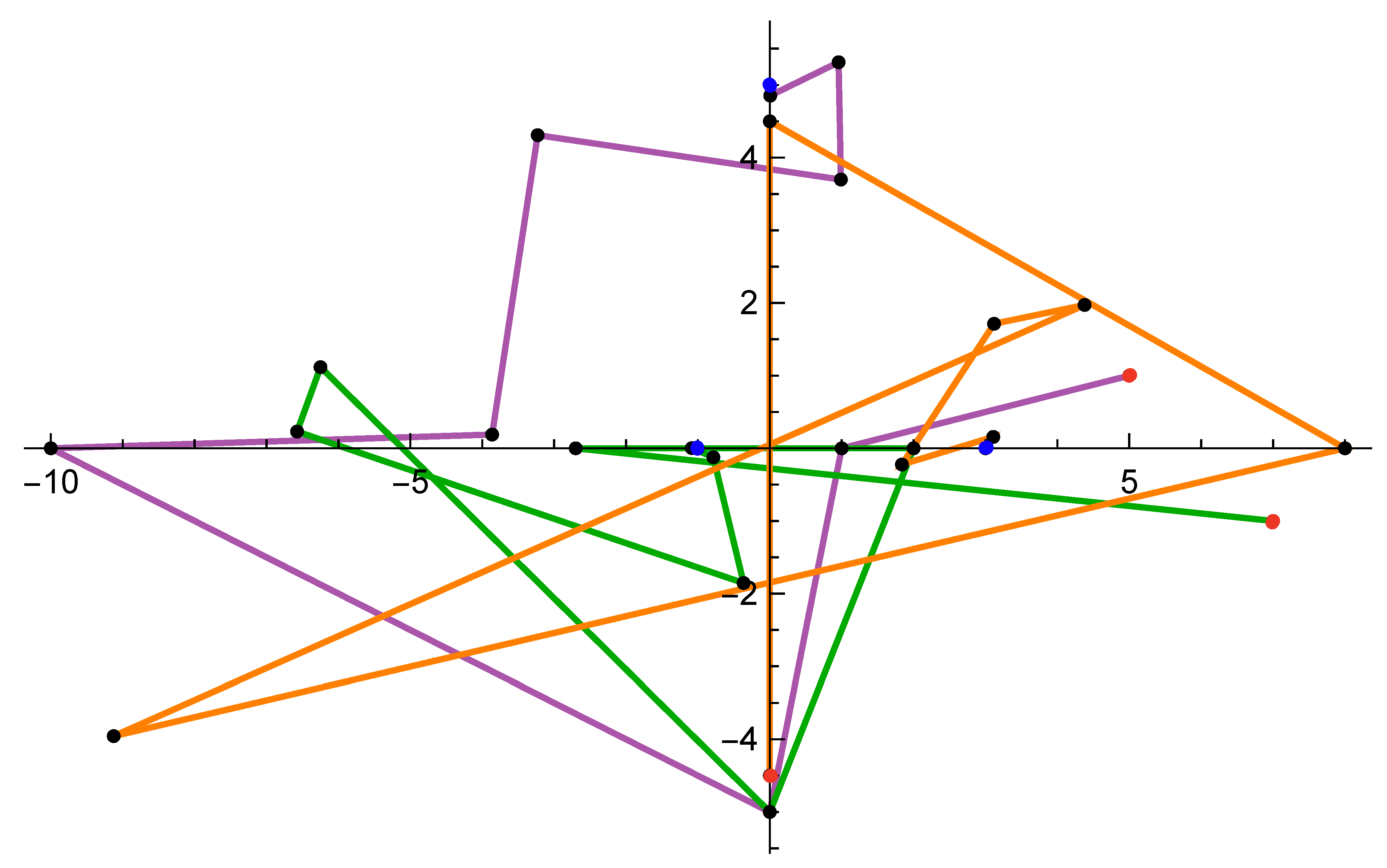
with zeros $-1$, 3 and $5i$ (marked in blue in Figure 1). For $N\in \{1,2,3,4\}$, the initial approximations $x^{\left(0\right)},x^{(-1)},\cdots ,x^{(-N)}$ in ${\mathbb{C}}^3$ are given in

Table 2. Initial approximations for Example 1.

N	${\mathit{x}}^{(-4)}$	${\mathit{x}}^{(-3)}$	${\mathit{x}}^{(-2)}$	${\mathit{x}}^{(-1)}$	${\mathit{x}}^{\left(0\right)}$
1	−	−	−	a	b
2	−	−	a	b	c
3	−	a	b	c	u
4	a	b	c	u	v

, where

$$a=(5+i,7-i,-4.5i),b=(1,-2.7,4.5i),c=(-5i,2,8),$$

$$u=(-10,-5i,8),v=(i,3+i,8).$$

In the case $N=3$, the initial approximations are marked in red in Figure 1.

The numerical results for Example 1 are presented in

Table 3. Convergence behavior for Example 1  ($R_n=0.125,{\tau }_n=0.171573$).

N	m	${\mathit{E}}_{\mathit{f}}\left({\mathit{x}}^{\left(\mathit{m}\right)}\right)$	k	${\mathit{E}}_{\mathit{f}}\left({\mathit{x}}^{\left(\mathit{k}\right)}\right)$	${\mathit{\epsilon }}_{\mathit{k}}$	${\mathit{\epsilon }}_{\mathit{k}+1}$	r
1	4	$0.036247$	5	$0.000039$	$9.06336\times {10}^{-14}$	$1.52321\times {10}^{-32}$	$2.41421$
2	5	$0.001957$	5	$0.001957$	$5.97453\times {10}^{-17}$	$5.45631\times {10}^{-48}$	$2.83117$
3	6	$0.076062$	6	$0.076062$	$2.46336\times {10}^{-16}$	$1.05897\times {10}^{-47}$	$2.94771$
4	7	$0.083021$	7	$0.083021$	$6.50717\times {10}^{-17}$	$3.80803\times {10}^{-51}$	$2.98314$

. For instance, for the multi-point Ehrlich-type method (11) with $N=3$, one can see that the convergence condition (51) is satisfied for $m=6$ which guarantees that the considered method is convergent with order of convergence $r=2.94771$. The stopping criterion (55) is satisfied for $k=6$ and at the sixth iteration the guaranteed accuracy is ${10}^{-16}$. At the next seventh iteration, the zeros of the polynomial f are calculated with accuracy ${10}^{-47}$.

In Figure 1, we present the trajectories of the approximations generated by the first six iterations of the method (11) for $N=3$. We observe how each initial approximation, moving along a bizarre trajectory, finds a zero of the polynomial.

Example 2.

The second polynomial is

$$f\left(z\right)=z^7-28z^6+322z^5-1960z^4+6769z^3-13132z^2+13068z-5040$$

(57)

with zeros $1,2,3,4,5,6,7$ (marked in blue in Figure 2). For given $N\in \{1,2,3,4\}$, the initial approximations $x^{\left(k\right)}\in {\mathbb{C}}^n$$(k=-N,\dots ,-1,0)$ are chosen with Aberth initial approximations as follows:

$$x_{\nu }^{\left(k\right)}=-\frac{a_1}{n}+R_{k}exp\left(i{\theta }_{\nu }\right),{\theta }_{\nu }=\frac{\pi }{n}\left(2\nu -\frac{3}{2}\right),\nu =1,\dots ,n,$$

(58)

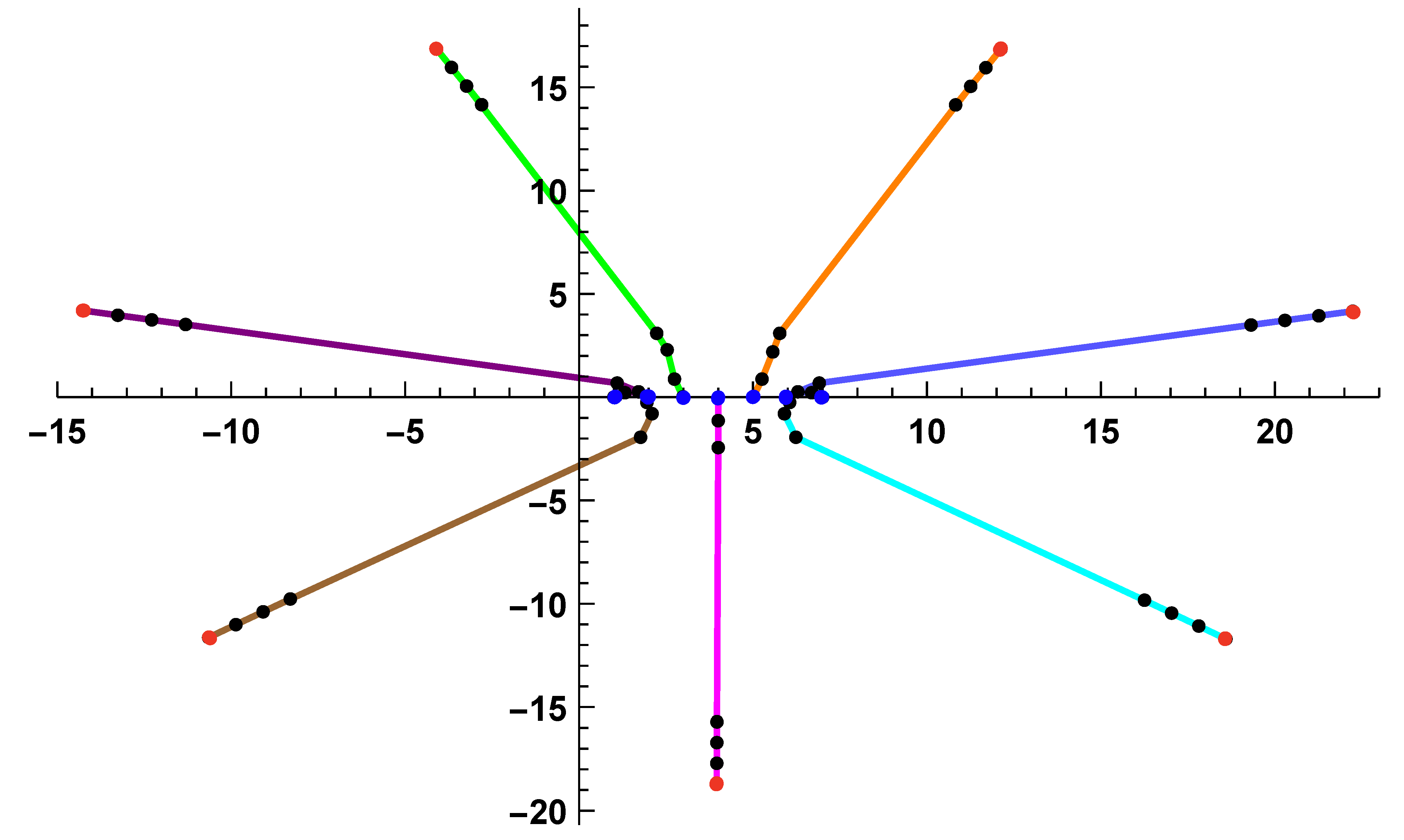
where $a_1=-28$, $n=7$, $R_k=R+2-k$ and $R=13.7082$. In the case $N=3$, the initial approximations are marked in red in Figure 2.

The numerical results for Example 2 are presented in

Table 4. Convergence behavior for Example 2  ($R_n=0.125,{\tau }_n=0.171573$).

N	m	${\mathit{E}}_{\mathit{f}}\left({\mathit{x}}^{\left(\mathit{m}\right)}\right)$	k	${\mathit{E}}_{\mathit{f}}\left({\mathit{x}}^{\left(\mathit{k}\right)}\right)$	${\mathit{\epsilon }}_{\mathit{k}}$	${\mathit{\epsilon }}_{\mathit{k}+1}$
1	18	$0.00526$	21	$3.48544\times {10}^{-10}$	$4.73454\times {10}^{-16}$	$1.25695\times {10}^{-38}$
2	6	$0.01689$	8	$7.85062\times {10}^{-6}$	$4.23967\times {10}^{-17}$	$1.06658\times {10}^{-48}$
3	7	$0.01348$	8	$0.00038$	$1.12167\times {10}^{-22}$	$6.66169\times {10}^{-65}$
4	14	$0.03215$	14	$0.03215$	$6.61642\times {10}^{-24}$	$4.98369\times {10}^{-71}$

. For example, for the multi-point Ehrlich-type method (11) with $N=3$, the convergence condition (51) is satisfied for $m=7$ and the stopping criterion (55) is satisfied for $k=8$ which guarantees an accuracy ${10}^{-22}$. At the next ninth iteration, the zeros of the polynomial f are calculated with accuracy ${10}^{-65}$. In Figure 1, we present the trajectories of the approximations generated by the first seven iterations of the method (11) for $N=3$. One can see that the trajectories are quite regular in the case of Aberth’s initial approximations.

7. Conclusions

In this paper, we introduced a new family of multi-points iterative methods for approximating all the zeros of a polynomial simultaneously. Let us note that the first member of this family is the two-point Ehrlich-type method introduced in 1999 by Trićković and Petković [9]. Its convergence order is $r=1+\sqrt{2}$.

We provide a local and semilocal convergence analysis of the new iterative methods. Our local convergence result (Theorem 2) contains the following information for each method: convergence order; initial conditions that guarantee the convergence; a priori and a posteriori error estimates. In particular, each method of the family has super-quadratic convergence of order $r\in [1+\sqrt{2},3)$. Our semilocal convergence result (Theorem 4) can be used to numerically prove the convergence of each method for a given polynomial and initial approximation.

Finally, we would like to note that the local convergence theorem was obtained by a new approach developed in our previous article [11]. We believe that this approach can be applied to obtain convergence results for other multi-point iterative methods.

References

- Stewart, G.W. On the convergence of multipoint iterations. Numer. Math. 1994, 68, 143–147. [Google Scholar] [CrossRef] [Green Version]
- Abu-Alshaikh, I.; Sahin, A. Two-point iterative methods for solving nonlinear equations. Appl. Math. Comput. 2006, 182, 871–878. [Google Scholar] [CrossRef]
- Ignatova, B.; Kyurkchiev, N.; Iliev, A. Multipoint algorithms arising from optimal in the sense of Kung-Traub iterative procedures for numerical solution of nonlinear equations. Gen. Math. Notes 2011, 11, 45–79. [Google Scholar]
- Argyros, I.K.; González, D. Unified majorizing sequences for Traub-type multipoint iterative procedures. Numer. Algorithms 2013, 64, 549–565. [Google Scholar] [CrossRef]
- Tiruneh, A.T.; Ndlela, W.N.; Nkambule, S.J. A two-point Newton method suitable for nonconvergent cases and with super-quadratic convergence. Adv. Numer. Anal. 2013, 687382. [Google Scholar] [CrossRef] [Green Version]
- Petković, M.S.; Neta, B.; Petković, L.D.; Džunić, J. Multipoint methods for solving nonlinear equations: A survey. Appl. Math. Comput. 2014, 226, 635–660. [Google Scholar] [CrossRef] [Green Version]
- Amat, S.; Argyros, I.; Busquier, S.; Hernández-Verón, M.A.; Rubio, M.J. A unified convergence analysis for some two-point type methods for nonsmooth operators. Mathematics 2019, 7, 701. [Google Scholar] [CrossRef] [Green Version]
- Kanno, S.; Kjurkchiev, N.V.; Yamamoto, T. On some methods for the simultaneous determination of polynomial zeros. Jpn. J. Indust. Appl. Math. 1996, 13, 267–288. [Google Scholar] [CrossRef]
- Tričković, S.B.; Petković, M.S. Multipoint methods for the determination of multiple zeros of a polynomial. Novi Sad J. Math. 1999, 29, 221–233. [Google Scholar]
- Proinov, P.D.; Petkova, M.D. Convergence of the two-point Weierstrass root-finding method. Jpn. J. Indust. Appl. Math. 2014, 31, 279–292. [Google Scholar] [CrossRef]
- Proinov, P.D.; Petkova, M.D. Local and semilocal convergence of a family of multi-point Weierstrass-type root-finding methods. Mediterr. J. Math. 2020, 17, 107. [Google Scholar] [CrossRef]
- Weierstrass, K. Neuer Beweis des Satzes, dass jede ganze rationale Function einer Veränderlichen dargestellt werden kann als ein Product aus linearen Functionen derselben Veränderlichen. Sitzungsber. Königl. Akad. Wiss. Berlin 1891, II, 1085–1101. [Google Scholar] [CrossRef]
- Ehrlich, L. A modified Newton method for polynomials. Commun. ACM 1967, 10, 107–108. [Google Scholar] [CrossRef]
- Aberth, O. Iteration methods for finding all zeros of a polynomial simultaneously. Math. Comput. 1973, 27, 339–344. [Google Scholar] [CrossRef]
- Börsch-Supan, W. Residuenabschätzung für Polynom-Nullstellen mittels Lagrange-Interpolation. Numer. Math. 1969/70, 14, 287–296. [Google Scholar] [CrossRef]
- Werner, W. On the simultaneous determination of polynomial roots. In Iterative Solution of Nonlinear Systems of Equations (Oberwolfach, 1982); Springer: Berlin, Germany; New York, NY, USA, 1982; Volume 953, pp. 188–202. [Google Scholar]
- Proinov, P.D.; Vasileva, M.T. On the convergence of high-order Ehrlich-type iterative methods for approximating all zeros of a polynomial simultaneously. J. Inequal. Appl. 2015, 2015, 336. [Google Scholar] [CrossRef]
- Proinov, P.D. General convergence theorems for iterative processes and applications to the Weierstrass root-finding method. J. Complex. 2016, 33, 118–144. [Google Scholar] [CrossRef]
- Proinov, P.D. Relationships between different types of initial conditions for simultaneous root finding methods. Appl. Math. Lett. 2016, 52, 102–111. [Google Scholar] [CrossRef]
- Proinov, P.D.; Ivanov, S.I. Convergence analysis of Sakurai-Torii-Sugiura iterative method for simultaneous approximation of polynomial zeros. J. Comput. Appl. Math. 2019, 357, 56–70. [Google Scholar] [CrossRef]
- Cholakov, S.I.; Vasileva, M.T. A convergence analysis of a fourth-order method for computing all zeros of a polynomial simultaneously. J. Comput. Appl. Math. 2017, 321, 270–283. [Google Scholar] [CrossRef]
- Ivanov, S.I. A unified semilocal convergence analysis of a family of iterative algorithms for computing all zeros of a polynomial simultaneously. Numer. Algorithms 2017, 75, 1193–1204. [Google Scholar] [CrossRef]
Figure 1.
Trajectories of the approximations for Example 1 ().
Figure 2.
Trajectories of the approximations for Example 2 ().