
Adaptation of Random Binomial Graphs for Testing Network Flow Problems Algorithms


Department of Mathematics and Computer Science, Faculty of Mathematics and Computer Science, Transilvania University of Brasov, 50003 Brașov, Romania
*
Author to whom correspondence should be addressed.
Mathematics 2021, 9(15), 1716; https://0-doi-org.brum.beds.ac.uk/10.3390/math9151716
Submission received: 29 June 2021
/
Revised: 16 July 2021
/
Accepted: 20 July 2021
/
Published: 21 July 2021
(This article belongs to the Special Issue Graph Theoretic Concepts in Data Science)
Abstract
:Algorithms for network flow problems, such as maximum flow, minimum cost flow, and multi-commodity flow problems, are continuously developed and improved, and so, random network generators become indispensable to simulate the functionality and to test the correctness and the execution speed of these algorithms. For this purpose, in this paper, the well-known Erdős–Rényi model is adapted to generate random flow (transportation) networks. The developed algorithm is fast and based on the natural property of the flow that can be decomposed into directed elementary s-t paths and cycles. So, the proposed algorithm can be used to quickly build a vast number of networks as well as large-scale networks especially designed for s-t flows.
1. Introduction
There are many applications of the network flow problems, e.g., electrical, water, or gas supply networks, vehicle routing and transportation, wireless networks, data mining, airline scheduling, project selection, image segmentation, network reliability, multi-camera scene reconstruction, security of statistical data, gene function prediction, open-pit mining, distributed computing, network connectivity, network intrusion detection, finance models, baseball elimination, etc., [1,2]. Algorithms for network flow problems are continuously developed and improved. Consequently, it is very important to have a tool for creating networks for testing the correctness and to compare the execution time of the new algorithms with the existing ones.
In the literature, a few methods used to build random graphs are proposed. Erdõs and Rényi introduced random binomial graphs in [3]. These random graphs are generated based on the values of two parameters: n (the number of nodes) and p ∈ [0, 1] (the probability of introducing any edge in the graph). These kinds of random networks have been applied for Zagreb indices, general sum-connectivity index, general inverse sum indeg index, and general first geometric-arithmetic index [4]. In a network generated in this manner, there is the possibility that the source will poorly communicate to the sink or even not communicate at all. An algorithm for generating simple random graphs with a given degree sequence was developed in [5]. Using this algorithm, an asymptotically uniform random graph with a given degree sequence is very quickly generated (almost linear time). In Reference [6], Barabási and Albert introduced their model (BA) consisting of an algorithm based on the preferential attachment mechanism for generating random scale-free networks. The networks generated this manner have real application on the Internet, citation networks, the World Wide Web, and some social networks. The algorithm starts with a network having m0 given nodes. Sequentially, nodes are introduced into the network. Each of these newly added nodes is connected to m ≤ m0 existing nodes using a given probability that is proportional to the number of connections that the previously added nodes already had. The probability pi of connecting a new node to node i is:
where ki is the so-called degree of node i. The denominator from Equation (1) is twice the existing number of edges from the network.
Penrose, M. introduced a so-called random geometric graph (RGG), which is an undirected geometric graph with randomly sampled nodes. To generate such a graph, a uniform distribution of the underlying space [0, 1)d is used, where d is the dimension of the space [7]. The idea behind generating a RGG is that two nodes are linked only if the distance between them is less than a given parameter r ∈ (0, 1). Therefore, r and n give the way a RGG is generated. Very recently, RGGs have been successfully applied in nanomaterials [8]. Waxman generalized RGGs by considering a probabilistic connection function [9].
Considering the fact that the existing results from the literature about network graphs are dealing with specific graphs that are not general enough, or not suitable for network flow problems, in this paper, a new idea for generating random networks is proposed that has the advantages of being fast and based on the natural property of the flow that can be decomposed into directed elementary paths and cycles. Consequently, the networks generated in this manner are suitable for testing the correctness and the time efficiency of algorithms for network flow problems such as minimum cost flow, maximum flow, multi-commodity flow problem, etc. The maximum flow problem is to find a flow from source to sink having the maximum possible value. Very recently, better and better algorithms were developed to solve this problem [10,11,12]. Together with maximum flow, the minimum cut can also be calculated [13]. The minimum cost flow is to find a flow having minimum cost from supply nodes to demand nodes. Recently, the best-known algorithm was developed for solving this problem [14]. The multi-commodity flow problem uses flow demands, or multiple commodities between different source nodes and sink nodes. The best currently known algorithm to solve this problem is from Karakostas [15]. There exist other flow problems of which the algorithms can still be improved, e.g., the inverse generalized maximum flow problems under sum-type distances, which are proved to be NP-hard [16].
In this paper, the Erdős–Rényi model is adapted to generate random flow networks. The paper is organized as follows. The flow decomposition into directed s-t path and directed cycles is presented in Section 2. An algorithm for generating random networks is deduced. The more general case of networks having multiple sources and sinks is also studied. The algorithm is tested both on CPU and CUDA in Section 3. In Section 4, some conclusions are discussed.
2. Algorithms for Generating Random Flow Networks
2.1. Flow Decomposition into Elementary Flows
Let G = (V, E, s, t, u, c) be an s-t directed network. V is a set containing n > 0 vertices (nodes), and E is a set of m ≥ 0 so-called arcs (directed edges); each arc a = (i, j) ∈ E connects two nodes i and j from V, s is a special node called source, and t is a node called sink. In G, we define the capacity function and, respectively, the cost function . The value u(a) is the maximum flow that can be transported from node i to node j on the arc a = (i, j) ∈ E, and c(a) is the per unit cost of transportation of flow on the arc a.
A (feasible) flow in an s-t directed network is a function satisfying the boundary restrictions (2) and conservation conditions from (3).
A feasible flow f can be decomposed into two feasible flows, f1 and f2, and is denoted by f = f1 + f2, if f(a) = f1(a) + f2(a), ∀ a ∈ E.
P = (u1, u2, …, uk) is called a directed path in G if (ui, ui+1) ∈ E, ∀ i ∈ {1, 2, …, k − 1}, where k ≥ 2. A directed path is called elementary if it does not pass a node twice, i.e., ui ≠ uj, ∀ i, j ∈ {1, 2, …, k}, i ≠ j. A directed cycle is a directed path for which the first node is equal to the last one, i.e., C = (u1, u2, …, uk = u1) is a directed cycle. A directed cycle is elementary if it does not pass a node twice, except for the first node. A flow f is called elementary if it is 0 on all the arcs of the network except for the arcs of a directed s-t path or of a directed cycle, where it is equal to a value v > 0.
In Reference [13] the following flow theorem is presented:
Theorem 1.
Any feasible flow f can be decomposed into directed paths and directed cycles such that:
- (a)
- Every directed path with positive flow connects the source s to the sink t.
- (b)
- At most n + m directed paths and directed cycles have non-zero flow. Out of these, at most m cycles have non-zero flow.
Proof of Theorem 1.
The proof can be found in [13]. □
So, a direct consequence of Theorem 1 is that a flow can be decomposed into at most n + m elementary flows.
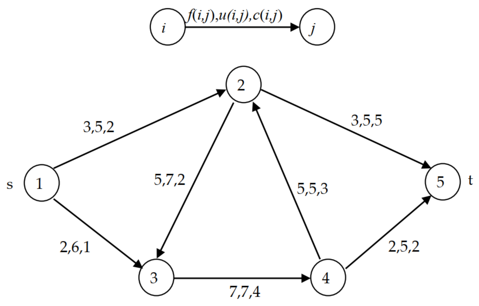
To illustrate the idea behind Theorem 1, in Figure 1, we present a flow f in a network G. The flow f is feasible since it satisfies both the conditions (2) and (3). The value of the flow f is vf = 5. One possible decomposition of the flow f into elementary flows is given by the f1, f2, and f3 flows corresponding, respectively, to the paths P1 = (1, 2, 5), P2 = (1, 3, 4, 5), and the cycle C = (2, 3, 4, 2). The value of the flow f1 is 3 and is equal to the value on the path P1. The value of the flow f2 is 2 and is equal to the value on the path P2. The value of the flow f3 is 0, but the value on the cycle C is equal to 5.
2.2. Algorithm for Generating Random s-t Flow Networks
Correctness and time efficiency comparisons of algorithms for network flow problems are important when new methods are elaborated. To do that, a fast and reliable tool is needed to generate random networks, starting with simple ones and continuing with large-scale networks. We develop a method based on the Erdős–Rényi model using the idea of Theorem 1 to create such a tool. Since a flow can be decomposed into elementary flows, a natural approach is to generate random directed elementary s-t paths and cycles.
We present now a first algorithm (Algorithm 1) to generate a random directed elementary s-t path:
| Algorithm 1. Algorithm Random s-t Directed Elementary Path v1 (ARDEP1) |
| /* source is considered having the first index, and sink is considered having the last one */ s = 0; t = n − 1; /* only source is initially part of the path */ for each node j other than s do pathnode[j] = false; end for; pathnode[s] = true; /* build the random path */ u = s; for j = 1 to n-1 do /* choose a random index k of the next node to be added to the path */ k = random(0, n–j-1); l = 0; /* find node v as the k-th node out of the not before chosen nodes */ for each node v do if pathnode[v] then continue; end if; if l = k then break; end if; l = l + 1; end for; /* add arc (u,v) to the network */ ma[u][v] = 1; /* mark node v as being part of path */ pathnode[v] = true; /* if the last node v added to the path is sink, then path is completed */ if v = t then break; end if; /* node u becomes v in order to prepare the adding of another node to the path */ u = v; end for; |
In ARDEP1, without restricting the generality of the algorithm, we consider the source’s index equal to 0, and n-1 as the index of the sink node t. The algorithm builds a path starting from s. At each iteration, a new node that was not previously added to the path is randomly selected and pushed at the end of the path. Each time a new node v is pushed back to the path, the arc (u, v) is added to the network, i.e., the value of the adjacency matrix ma is set to 1 on the position (u, v), where u is the node previously added to the path. The algorithm ends when the sink node is added to the path.
Next, we present Algorithm 2 to generate a random directed elementary cycle:
| Algorithm 2. Algorithm Random Directed Elementary Cycle v1 (ARDEC1) |
| /* choose a random node u0 */ u0 = random(0, n-1); /* only node u0 is initially part of the cycle */ for each node j other than u0 do cyclenode[j] = false; end for; cyclenode[s] = true; /* build the random cycle */ u = u0; for j = 0 to n-1 do /* choose a random index k of the next node to be added to the cycle */ k = random(0, n–j-1); l = 0; /* find node v as the k-th node out of the not before chosen nodes */ for each node v do if cyclenode[v] then continue; end if; if l = k then break; end if; l = l + 1; end for; /* if v is u then regenerate v. This can only happen when u = u0 */ if u = v then j = j – 1; else /* add arc (u,v) to the network */ ma[u][v] = 1; /* mark node v as being part of cycle */ cyclenode[v] = true; end if; /* if v is the first chosen node u0, then cycle is completed */ if v = u0 then break; end if; /* node u becomes v in order to prepare the adding of another node to the cycle */ u = v; end for; |
In ARDEC1, a cycle is built starting with a randomly chosen node u0. At each iteration, a new node that is not already part of the cycle is randomly selected and added to the cycle. Each time a new node v is introduced into the cycle, the arc (u, v) is also added to the network, where u is the node previously added to the cycle. The algorithm ends when the node u0 is added again to the cycle.
The algorithms ARDEP1 and ARDEC1 can naturally build directed elementary s-t paths and cycles. Their time complexity is obviously O(n2). These two algorithms could be used together to build random networks. However, we shall present a faster approach below.
Richard Durstenfeld proposes an algorithm to randomly generate a permutation [17]. In Algorithm 3, we propose a similar but simpler approach to generate a shuffled vector of nodes having the indexes between istart and iend:
| Algorithm 3. Algorithm Shuffled Vector of Nodes (ASVN) |
| Input: istart, iend; /* the vector “nodes” initially contains the indexes from istart to iend */ for j = istart to iend do nodes[j] = j; end for; /* shuffle the vector “nodes” */ for k = istart to iend do u = random(istart, iend); v = random(istart, iend); if u ≠ v then swap = nodes[u]; nodes[u] = nodes[v]; nodes[v] = swap; end if; end for; |
ASVN starts with a vector having all the nodes with indexes from istart to iend. Then, this vector is shuffled by two randomly chosen nodes from the vector and by interchanging their positions. These interchanges are executed n times, where n is the length of the vector. We have the following theorem that proves the quality of the obtained shuffled vector:
Theorem 2.
Using ASVN, any vector of the nodes randomly generated by ASVN has equal probability to be generated.
Proof of Theorem 2.
Let us suppose we have n values that have to be generated using ASVN. The initial vector of nodes contains n distinct values. There are n random swapping operations applied to the vector. We shall prove that any permutation of the initial values can be obtained this way.
Let p = (p1, p2, …., pn) be a permutation of the initial values istart, istart+1, …., iend. The following algorithm (Agorithm 4) transforms the initial vector nodes into p.
| Algorithm4. Algorithm Nodes Permutation (ANP) |
| /* generate the permutation pk of the nodes */ for k = 1 to n do Find the index i of pk in nodes; swap = nodes[i]; nodes[i] = nodes[k]; nodes[k] = swap; end for; |
Using ANP, there are n swapping operations that transform nodes into p. ASVN performs n random swapping operations to nodes. So, there always is a chance for ASVN to generate p from nodes. The probability to generate p from nodes is using ASVN, and, since the total number of possible permutations is n!, it results that any permutation of the vector nodes has an equal chance to be generated using ASVN. □
We now introduce two new methods to randomly generate directed elementary s-t paths and cycles using ASVN.
| Algorithm 5. Algorithm Random s-t Directed Elementary Path v2 (ARDEP2) |
| /* efficiently generate a shuffled vector of nodes without s and t */ ASVN(1, n-2); s = 0; t = n – 1; /* randomly generate the length of the path */ lpath = random(2, n); /* add the arcs given by the first lpath nodes of the shuffled vector to the network */ m_ma[s][nodes[1]] = 1; for k = 1 to lpath – 3 do m_ma[nodes[k]][nodes[k + 1]] = 1; end for; ma[nodes[lpath - 2]][t] = 1; |
In Algorithm 5, first, ARDEP2 randomly generates the length of the path. lpath-2 nodes are then taken from the shuffled vector of nodes, and together with source and sink, generate the path.
| Algorithm 6. Algorithm Random Directed Elementary Cycle v2 (ARDEC2) |
| /* efficiently generate a shuffled vector of nodes */ ASVN(0, n-1); /* randomly generate the length of the cycle */ lcycle = random(2, n); /* add the arcs given by the first lcycle nodes of the shuffled vector to the network */ for k = 0 to lcycle – 1 do m_ma[nodes[k]][nodes[k + 1]] = 1; end for; ma[nodes[lcycle - 1]][nodes[0]] = 1; |
In Algorithm 6, ARDEC2 takes lcycle nodes from the shuffled vector of nodes and generates a cycle.
Below, we introduce Algorithm 7 for generating a random flow network.
| Algorithm 7. Algorithm Generating Random s-t Flow Network (AGRFN) |
| Input: p, npath, ncycle, minu, maxu, minc, maxc; /* generate “npath” random paths */ for k = 1 to npath do ARDEP2; end for; /* generate “ncycle” random cycles */ for k = 1 to ncyle do ARDEC2; end for; /* generate the adjacency lists “la” using the adjacency matrix “ma” */ for i = 0 to n do la[i] = null; end for; /* randomly attach capacities and costs to the arcs when they are added to “la” */ for i = 0 to n do for j = 0 to n do /* generate arcs according to Erdős–Rényi model */ if ma[i][j] = 0 and random(0, 1000) < p*1000 then ma[i][j] = 1; end if; if ma[i][j] = 1 then Push back (j,random(minu,maxu),random(minc,maxc)) to la[i]; end if; end for; end for; |
Before starting AGRFN, the adjacency matrix ma is set to 0. The algorithm builds ma and then the adjacency lists la using ma.
After the directed s-t paths and directed cycles are built, arcs are randomly added to the network using the Erdős–Rényi model. According to this model, the probability of adding a new arc is p ∈ [0, 1]. Consequently, in AGRFN, for each pair of nodes (i, j), i ≠ j, so that ma[i, j] = 0, i.e., (i, j) is not currently an arc in the network, a random integer number is generated in the interval [0, 999] using the function random, and if this value is less then p ∙ 1000, the arc (i, j) is added to the network.
The capacities of the arcs are randomly generated between the given values minu and maxu. The costs on the arcs are also randomly generated between minc and maxc. There are more parameters for some flow problems such as lower bounds [13,18], modification limits for capacities [19,20], arc resistance [21,22], or gain factor [16,23]. These values can also be randomly generated on arcs.
Theorem 3.
The time complexity of AGRFN is O (n · max{npath, ncycle, n}).
Proof of Theorem 3.
For the time complexity of generating an s-t path or a cycle using ARDEP2, respectively, ARDEC2 is O(n). Consequently, the adjacency matrix ma is generated in O(max{npath, ncycle} · n), and since generating the adjacency lists takes O(n2) time, the time complexity of the algorithm is O(n · max{npath, ncycle, n}). □
Usually, it is enough to consider the number of paths and the number of cycles less than the number of nodes. So, in practice, the time complexity is likely to be O(n2).
The time complexity from Theorem 3 can be improved if the generation of the paths, cycles, and the adjacency lists are parallelized. The computations from the algorithm are elementary and they only involve integer values. So, AGRFN can be naturally parallelized on GPUs. Since the speed of generating of large-scale random networks is essential, time complexity improvement by parallelization can act an important role. Considering a total of g GPUs, the generation of the paths and cycles can be divided into max{1, (npath+ncycle)/g} groups. The generation of the adjacency lists can also be divided into max{1, n/g} groups. So, the time complexity of the parallel implementation on GPUs of AGRFN is O(n · max{npath, ncycle, n}/g).
The C++ source code for generating random networks using AGRFN can be found in Appendix A (Source code S1).
The network from Figure 2 was generated using AGRFN. The input parameters were as follows: p = 0.2, npath = 4, ncycle = 2, minu = 1, maxu = 7, minc = 1, and maxc = 7. The algorithm generated the following directed paths: P1 = (1, 2, 3, 6), P2 = (1, 6), P3 = (1, 4, 5, 6), and P4 = (1, 2, 4, 6), as well as the directed cycles C1 = (4, 5, 2, 3, 4), and C2 = (2, 4, 5, 1, 2). In the end, from the remaining 19 pairs of nodes were not connected with arcs, based on the considered probability of p = 0.2, and AGRFN generated three more arcs: (1, 5), (3, 4), and (3, 5).
2.3. The Case of Multiple Sources and Multiple Sinks
There are situations when networks having multiple source and sink nodes have to be generated. We shall show how AGRFN can be adapted for this more general case.
Let G = (V, E, S, T, u, c) be a directed network, where S = {s1, s2, …, sns} is the set of ns ≥ 1 sources and T = {t1, t2, …, tnt} is the set of nt ≥ 1 sink nodes. G is equivalent to an s-t network G’ = (V’, E’, s, t, u’, c’) by introducing a super-source s, a super-sink t, and the arcs (s, si) and (tj, t), where si ∈ S, i ∈ {1, 2, …, ns}, and tj ∈ T, j ∈ {1, 2, …, nt} [13]. The capacities and costs for the newly introduced arcs are irrelevant at this point. Using AGRFN, a random network G’ is built. In the end, the arcs (s, si) and (tj, t), where si ∈ S, i ∈ {1, 2, …, ns}, and tj ∈ T, j ∈ {1, 2, …, nt} are eliminated together with the nodes s and t, so that a random network G with multiple source and sink nodes is randomly generated.
| Algorithm 8. Algorithm Generating Random Network Multiple Sources and Sinks (AGRFNMSS) |
| Input: p, npath, ncycle, minu, maxu, minc, maxc; /* add super-source and super-sink nodes */ Add s and t to V; /* the adjacency matrix initially has no arcs */ ma = 0; /* connect super-source with the other sources */ for i = 1 to ns do ma[s][si] = 1; end for; /* connect super-sink with the other sinks */ for j = 1 to nt do ma[tj][t] = 1; end for; /* call AGRFN to generate a random netowrk */ AGRFN(p, npath, ncycle, minu, maxu, minc, maxc); /* come back to the initial network having multiple sources and sinks */ |
In Algorithm 8, the nodes s and t are eliminated from V, and the adjacency matrix ma is modified accordingly.
It is obvious that the time complexity of AGRFNMSS is the same as for AGRFN.
3. Results and Discussions
In Figure 3, three networks having 6, 20, and 100 nodes, respectively, were generated and displayed. For the first network, 3 paths and 2 cycles were generated. For the second network, 10 paths and 2 cycles were generated, and for the last network, 20 paths and 10 cycles were generated.
Different tests were performed to illustrate the generating time of increasing the scale of random networks having the number of nodes between 10 and 10,000. As expected, and as shown in Table 1, the number of nodes together with the number of considered paths and cycles directly influence the speed of the network generation. An Asus ROG Strix G17 G712LV, Intel Core i7-10750H up to 5.10 GHz processor, 16GB RAM, NVIDIA GeForce RTX 2060 6GB GDDR6 with 1920 CUDA cores was used. The tests showed that the usage of parallelization becomes more and more effective with the increase of the dimension of the networks. The parallelization was implemented using CUDA programming on GPU. Each path and cycle were created on a different thread. Additionally, the creation of adjacency lists from the adjacency matrix was parallelized, the list for each node being obtained on a different thread. For small networks (less than 50 nodes) it is better to use the implementation of the algorithm on CPU, but when the number of the nodes of the networks is more than 50, the CUDA implementation is preferred resulting in a clear speed-up, up to 19 times faster than the CPU implementation. The speed-up was calculated as the ratio between CUDA and CPU execution times. The best speed-up was obtained for large-scale networks having thousands of nodes (Table 1).
In Figure 4, the speed-up evolution for generating networks of different dimensions is presented.
4. Conclusions
We developed a fast and reliable algorithm called AGRFN to randomly generate networks. The resulted networks can be used to test the correctness and efficiency of algorithms developed for network flow problems, e.g., minimum cost flow, maximum flow, or multi-commodity flow problems. The CUDA parallelized version of AGRFN proved to be up to 19 times faster when large-scale networks need to be generated.
Considering further developments, other problems in specific networks could be identified in which AGRFN can be adapted.
Author Contributions
Conceptualization, A.M.D.; methodology, A.M.D. and D.S.; software, A.M.D.; validation, D.S.; formal analysis, A.M.D. and D.S.; investigation, D.S.; resources, D.S.; data curation, D.S.; writing—original draft preparation, A.M.D. and D.S.; writing—review and editing, A.M.D. and D.S.; supervision, A.M.D.; funding acquisition, A.M.D. and D.S. All authors have read and agreed to the published version of the manuscript.
Funding
This research was funded by University Transilvania of Brașov.
Institutional Review Board Statement
Not applicable.
Informed Consent Statement
Not applicable.
Data Availability Statement
Not applicable.
Conflicts of Interest
The authors declare no conflict of interest.
Appendix A
| Source code S1: The C++ source code for generating random networks using AGRFN. |
| // The header file (“.h” file): #pragma once #include"vector" using namespace std; struct arc { // i = end node of the arc int i, u, c; // u = capacity of the arc }; // c = cost of the arc class NetworkCreation { vector<vector<int>> m_ma; // adjacency matrix vector<vector<arc>> m_la; // adjacency lists void CreateLAFromMA(float p, int mincap, int maxcap, int mincost, int maxcost); public: NetworkCreation(float p, int nnod, int npath, int ncycle, int mincap, int maxcap, int mincost, int maxcost); vector<vector<int>>& GetMA(); vector<vector<arc>>& GetLA(); }; // The implementations (“.cpp” file): #include"NetworkCreation.h" #include"time.h" void NetworkCreation::CreateLAFromMA(float p, int mincap, int maxcap, int mincost, int maxcost) { int nnod = m_ma.size(); if (!nnod) return; m_la.resize(nnod); int u, c; for (int i = 0; i < nnod; i++) for (int j = 0; j < nnod; j++) { if (!m_ma[i][j] && rand() % 1000 < p * 1000) m_ma[i][j] = 1; if (m_ma[i][j]) { u = maxcap; if (mincap < maxcap) u = rand() % (maxcap - mincap + 1) + mincap; c = maxcost; if (mincost < maxcost) c = rand() % (maxcost - mincost + 1) + mincost; m_la[i].push_back({ j,u,c }); } } } NetworkCreation::NetworkCreation(float p, int nnod, int npath, int ncycle, int mincap, int maxcap, int mincost, int maxcost) { if (nnod < 2) return; m_ma.resize(nnod); for (int i = 0; i < nnod; i++) { m_ma[i].resize(nnod); for (int& k : m_ma[i]) k = 0; } srand(time(0)); int s = 0, t = nnod - 1; // randomly generate paths for (int i = 0; i < npath; i++) { vector<int> generate(nnod - 2); for (int k = 0; k < nnod - 2; k++) generate[k] = k + 1; // shuffle nodes for (int k = 0; k < nnod - 2; k++) { int u = rand() % (nnod - 2); int v = rand() % (nnod - 2); int swap = generate[u]; generate[u] = generate[v]; generate[v] = swap; } // generate random path int lpath = rand() % (nnod - 2) + 1; m_ma[s][generate[0]] = 1; for (int k = 0; k < lpath - 1; k++) m_ma[generate[k]][generate[k + 1]] = 1; m_ma[generate[lpath - 1]][t] = 1; } // randomly generate cycles for (int i = 0; i < ncycle; i++) { vector<int> generate(nnod); for (int k = 0; k < nnod; k++) generate[k] = k; // shuffle nodes for (int k = 0; k < nnod; k++) { int u = rand() % (nnod); int v = rand() % (nnod); int swap = generate[u]; generate[u] = generate[v]; generate[v] = swap; } // generate random cycle int lcycle = rand() % nnod + 1; for (int k = 0; k < lcycle - 1; k++) m_ma[generate[k]][generate[k + 1]] = 1; m_ma[generate[lcycle - 1]][generate[0]] = 1; } CreateLAFromMA(p, mincap, maxcap, mincost, maxcost); } vector<vector<int>>& NetworkCreation::GetMA() { return m_ma; } vector<vector<arc>>& NetworkCreation::GetLA() { return m_la; } |
References
- Mahmoudi, M.; Boloori, A. Network Flow Applications, in Graph Theory for Operations Research and Management: Applications in Industrial Engineering; IGI Global: Hershey, PA, USA, 2013; pp. 246–256. [Google Scholar]
- Bingdong, L.; Springer, J.; Bebis, G.; Gunes, M.H. A survey of network flow applications. J. Netw. Comput. Appl. 2013, 36, 567–581. [Google Scholar]
- Erdõs, P.; Rényi, A. On Random Graphs. I. Publ. Math 1959, 6, 290–297. [Google Scholar]
- Cuadra, L.; Nieto-Borge, J.C. Modeling Quantum Dot Systems as Random Geometric Graphs with Probability Amplitude-Based Weighted Links. Nanomaterials 2021, 11, 375. [Google Scholar] [CrossRef] [PubMed]
- Bayati, M.; Kim, J.H.; Saberi, A. A Sequential Algorithm for Generating Random Graphs. Algorithmica 2010, 58, 860–910. [Google Scholar] [CrossRef] [Green Version]
- Réka, A.; Barabási, A.L. Statistical mechanics of complex networks. Rev. Mod. Phys. 2002, 74, 47–97. [Google Scholar]
- Penrose, M. Random Geometric Graphs; Oxford University Press: Oxford, UK, 2003; ISBN 13 9780198506263. [Google Scholar]
- Aguilar-Sánchez, R.; Herrera-González, I.F.; Méndez-Bermúdez, J.A.; Sigarreta, J.M. Computational Properties of General Indices on Random Networks. Symmetry 2020, 12, 1341. [Google Scholar] [CrossRef]
- Waxman, B.M. Routing of multipoint connections. IEEE J. Sel. Areas Commun. 1988, 6, 1617–1622. [Google Scholar] [CrossRef]
- Orlin, J.B. Max flows in O(nm) time, or better. In Proceedings of the 45th annual ACM symposium on Symposium on Theory of Computing-STOC-’13, Palo Alto, CA, USA, 2–4 June 2013; pp. 765–774. [Google Scholar]
- Brand, J.; Lee, Y.T.; Nanongkai, D.; Peng, R.; Saranurak, T.; Sidford, A.; Song, Z.; Wang, D. Bipartite Matching in Nearly-linear Time on Moderately Dense Graphs. In Proceedings of the IEEE 61st Annual Symposium on Foundations of Computer Science (FOCS), Durham, NC, USA, 16–19 November 2020; pp. 919–930. [Google Scholar]
- Gao, Y.; Liu, Y.P.; Peng, R. Fully Dynamic Electrical Flows: Sparse Maxflow Faster Than Goldberg-Rao. arXiv 2021, arXiv:2101.07233. [Google Scholar]
- Ahuja, R.K.; Magnanti, T.L.; Orlin, J.B. Network Flows: Theory, Algorithms, and Applications; Prentice Hall: Englewood Cliffs, NJ, USA, 1993. [Google Scholar]
- Yongwen, H.; Xiao, Z.; Jing, L.; Binyuan, L.; Chao, M. An Efficient Algorithm for Solving Minimum Cost Flow Problem with Complementarity Slack Conditions. Math. Probl. Eng. 2020, 2020. [Google Scholar] [CrossRef]
- Karakostas, G. Faster approximation schemes for fractional multicommodity flow problems. In Proceedings of the 13th Annual ACM-SIAM Symposium on Discrete Algorithms, San Francisco, CA, USA, 6–8 January 2002; pp. 166–173. [Google Scholar]
- Tayyeby, J.; Deaconu, A.M. Inverse Generalized Maximum Flow Problems. Mathematics 2019, 7, 899. [Google Scholar] [CrossRef] [Green Version]
- Durstenfeld, R. Algorithm 235: Random permutation. Commun. ACM 1964, 7, 420. [Google Scholar] [CrossRef]
- Deaconu, A.; Ciupala, L. Inverse Minimum Cut Problem with Lower and Upper Bounds. Mathematics 2020, 8, 1494. [Google Scholar] [CrossRef]
- Deaconu, A.; Ciurea, E. The inverse maximum flow problem under Lk norms, Carpathian. J. Math. 2012, 28, 59–66. [Google Scholar]
- Deaconu, A. A Cardinality Inverse Maximum Flow Problem. Sci. Ann. Cuza Univ. 2006, 16, 51–62. [Google Scholar]
- Marinescu, C.; Deaconu, A.; Ciurea, E.; Marinescu, D. From microgrids to smart grids: Modeling and simulating using graphs. Part I active power flow, OPTIM 2010. In Proceedings of the 12th International Conference on Optimization of Electrical and Electronic Equipment, Brasov, Romania, 20–22 May 2010; pp. 1245–1250. [Google Scholar]
- Marinescu, C.; Deaconu, A.; Ciurea, E.; Marinescu, D. From Microgrids to Smart Grids: Modeling and Simulating using Graphs. Part II Optimization of Reactive Power Flow, OPTIM 2010. In Proceedings of the 12th International Conference on Optimization of Electrical and Electronic Equipment, Brasov, Romania, 20–22 May 2010; pp. 1251–1256. [Google Scholar]
- Sven, O.K.; Zeck, C. Generalized max flow in series-parallel graphs. Discret. Optim. 2013, 10, 155–162. [Google Scholar]
Figure 1.
A network G and a flow f.

Figure 2.
Network generated with AGRFN.

Figure 3.
Networks generated using AGRFN. (a) Network with n = 6, npath = 3, ncycle=2; (b) network with n = 20, npath = 10, ncycle = 2; (c) network with n = 100, npath = 20, ncycle = 10.
Figure 3.
Networks generated using AGRFN. (a) Network with n = 6, npath = 3, ncycle=2; (b) network with n = 20, npath = 10, ncycle = 2; (c) network with n = 100, npath = 20, ncycle = 10.

Figure 4.
Speed-up CUDA/CPU.


Table 1.
Random network generation and running time comparison.
| No. of Networks | No. of Nodes | No. of Paths | No. of Cycles | CPU Time (Seconds) | CUDA Time (Seconds) | No. of Blocks | Threads Per Block | Speed-Up |
|---|---|---|---|---|---|---|---|---|
| 1,000,000 | 10 | 5 | 2 | 8.42 | 69.50 | 1 | 10 | 0.12 |
| 100,000 | 50 | 20 | 10 | 14.39 | 10.99 | 1 | 50 | 1.31 |
| 50,000 | 100 | 50 | 25 | 31.33 | 8.64 | 1 | 100 | 3.62 |
| 4000 | 500 | 200 | 100 | 44.66 | 6.10 | 1 | 500 | 7.32 |
| 1000 | 1000 | 500 | 250 | 55.33 | 4.09 | 1 | 1000 | 13.54 |
| 50 | 5000 | 2000 | 1000 | 58.19 | 3.20 | 5 | 1000 | 18.16 |
| 10 | 10,000 | 5000 | 2500 | 57.33 | 3.01 | 10 | 1000 | 19.05 |
Publisher’s Note: MDPI stays neutral with regard to jurisdictional claims in published maps and institutional affiliations. |
© 2021 by the authors. Licensee MDPI, Basel, Switzerland. This article is an open access article distributed under the terms and conditions of the Creative Commons Attribution (CC BY) license (https://creativecommons.org/licenses/by/4.0/).
Share and Cite
MDPI and ACS Style
Deaconu, A.M.; Spridon, D. Adaptation of Random Binomial Graphs for Testing Network Flow Problems Algorithms. Mathematics 2021, 9, 1716. https://0-doi-org.brum.beds.ac.uk/10.3390/math9151716
AMA Style
Deaconu AM, Spridon D. Adaptation of Random Binomial Graphs for Testing Network Flow Problems Algorithms. Mathematics. 2021; 9(15):1716. https://0-doi-org.brum.beds.ac.uk/10.3390/math9151716
Chicago/Turabian StyleDeaconu, Adrian Marius, and Delia Spridon. 2021. "Adaptation of Random Binomial Graphs for Testing Network Flow Problems Algorithms" Mathematics 9, no. 15: 1716. https://0-doi-org.brum.beds.ac.uk/10.3390/math9151716
Note that from the first issue of 2016, this journal uses article numbers instead of page numbers. See further details here.