Modelling Interaction Effects by Using Extended WOE Variables with Applications to Credit Scoring

Abstract

The term credit scoring refers to the application of formal statistical tools to support or automate loan-issuing decision-making processes. One of the most extended methodologies for credit scoring include fitting logistic regression models by using WOE explanatory variables, which are obtained through the discretization of the original inputs by means of classification trees. However, this Weight of Evidence (WOE)-based methodology encounters some difficulties in order to model interactions between explanatory variables. In this paper, an extension of the WOE-based methodology for credit scoring is proposed that allows constructing a new kind of WOE variable devised to capture interaction effects. Particularly, these new WOE variables are obtained through the simultaneous discretization of pairs of explanatory variables in a single classification tree. Moreover, the proposed extension of the WOE-based methodology can be complemented as usual by balance scorecards, which enable explaining why individual loans are granted or not granted from the fitted logistic models. Such explainability of loan decisions is essential for credit scoring and even more so by taking into account the recent law developments, e.g., the European Union’s GDPR. An extensive computational study shows the feasibility of the proposed approach that also enables the improvement of the predicitve capability of the standard WOE-based methodology.

1. Introduction

Until the end of the 1960s, most decision making regarding loan granting was still based on traditional human subjective assessments. However, because of the growth of the credit card business at that time period, banks began to increasingly rely on automatic decision processes, giving rise to the notion and practice of credit scoring. As discussed in [1], this notion was fully recognized in the USA by the 1975 Equal Opportunity Act, which stated that any discrimination can be based only on statistical assessments.

Technically, credit scoringis the term used to describe formal statistical methods used for classifying applicants for credit into ’good’ and ’bad’ risk classes [2]. As described in this last work, the standard statistical methods used in the industry for developing scorecards are discriminant analysis, logistic regression and decision trees, mainly because of their ease of interpretation. Among these, the first two have been the most widely used techniques. The work in [3] provides one of the first published accounts of logistic regression applied to credit scoring in a comparison with discriminant analysis. It concludes that the logistic approach obtained superior classification results.

More recent works such as, e.g., [4,5], make reference to the application of sophisticated machine learning (ML) techniques in the credit scoring context, such as (again) neural networks, support vector machines (SVM), or widely extended model-ensemble techniques such as random forest and extreme gradient boosting or stacking, among others. Nevertheless, despite these recent applications, an actual consensus does not currently exist regarding the convenience of applying sophisticated ML methods in the credit scoring field. As discussed in [6], some studies have found that statistical techniques perform better than some ML techniques, such as neural networks or genetic algorithms, while other works concluded just the opposite. However, even if ML techniques outperform the predictive capability of statistical methods in this field, it is the interpretability of results that seems to mark the most important difference in favour of statistical methods. For instance, a direct consequence of the implementation since May 2018 of the European Union’s General Data Protection Regulation (GDPR, see [7]) is that banks need to be able to explain why a loan was not granted if the decision process was automatic, i.e., customers have the right to receive an explanation in the case of a negative credit decision (and see [8] for a wider discussion of the general implications of GDPR laws in algorithmic decision making).

With respect to this, one may argue that recent research in model interpretability techniques such as LIME (Local Interpretable Model-Interpretable Explanations, see [9,10]) may instead tip the scale in favour of ML-based solutions for credit scoring. Indeed, some recent works point at this direction (see, e.g., [11]). However, there is, again, no consensus regarding the general feasibility and convenience of such kinds of model interpretability techniques since an increasing amount of authors and works points that it may be more appropriate to further develop interpretable methods rather than to develop interpretability techniques to be applied upon black-box models [12].

Regarding the interpretability of the standard models of credit scoring, in the 1990s Kaplan and Norton developed balance scorecards [13]. In order to justify why loans are granted or not, the scorecards permitted an interpretation of a credit scoring model by detailing the amount of ‘points’ to be assigned to a client based on the values of each of the explanatory variables considered in such a decision model. The methodology underlying balance scorecards relies on fitting logistic regression models by using WOE (Weight Of Evidence, see [14]) variables as explanatory variables. These WOE variables, the definition and advantages of which will be reviewed in Section 2.3, are obtained by means of a transformation applied on the categories resulting from the discretization (typically by means of classification trees) of the original inputs. As discussed in [15], WOE transformations usually work well in logistic models not containing interaction terms and this lack of adaptation with respect to interacting variables is one of the main criticisms that may be made regarding the mentioned methodology.

A natural possibility to reflect interaction behaviours would consist in using products of WOE variables, since these present a continuous nature. However, as shall be discussed later in this work, such a standard procedure to model interactions presents some drawbacks in the case of WOE variables. This motivates our proposal of an alternative methodology to consider interaction effects in the context of credit scoring.

Specifically, the proposed methodology proceeds by fitting a classification tree to each pair of original input variables and applying a variant of the usual WOE transformation in order to generate a new typology of variables that shall be referred to as two-dimensional or, for simplicity, bivariate WOE variables. Let us stress that in this context the term bivariate just refers to the presence of two explanatory variables rather than to a bivariate target variable. These new variables can reflect interaction effects without resorting to products of usual WOE variables. In order to distinguish WOE variables using a single explanatory variable from the proposed bivariate WOE variables, the former shall be referred as univariate WOE variables. Furthermore, the standard scorecard methodology can be easily adapted to be apply on the proposed bivariate WOE variables, and thus these safeguard the typical interpretability tools of credit scoring.

Finally, in order to illustrate the feasibility of the proposed approach, a wide computational study has been carried out on a set of well-known reference datasets in the context of credit scoring. The results obtained by models using the proposed bivariate WOE methodology significantly improve on those of models based on the traditional univariate WOE approach.

This paper is organized as follows: Section 2 reviews the preliminary notions needed for the development of the proposed methodology, which is presented in Section 3. The configuration and results of the computational study carried out are described in Section 4. Some conclusions are then shed in Section 5. The paper also contains three appendices. Appendix A details the content of the dataset employed in the example exposed in Section 3.3, devoted to illustrating the application of the proposed methodology. Appendix B provides some considerations regarding some other reference datasets and the variables being used in the computational study. Appendix C illustrates the stepwise variable selection process involved in one of the model adjustments.

2. Preliminaries

This section is devoted to reviewing the main notions needed to present the proposed methodology for the generation of bivariate WOE variables.

With this aim in mind, Section 2.1 recalls some of the basics of logistic regression models, discussing pros and cons of discretizing the explanatory variables being considered. Next, Section 2.2 reviews the notion of interaction between variables in such models. Finally, Section 2.3 recalls the definition of (univariate) WOE variables.

2.1. Logistic Regression

Logistic regression is a widely used tool to model binary events, such as credit defaulting, in an interpretable manner. Denoting by Y the binary target variable ($Y=1$ if the loan is defaulted and $Y=0$ otherwise) and assuming a single explanatory variable X, the logistic model relies upon using the logistic function (Equation (1)) as the linkage function of a generalized linear model.

$$\pi \left(x\right)={\displaystyle \frac{1}{1+e^{-({\beta }_0+{\beta }_1·x)}}}$$

(1)

Function $\pi \left(x\right)$ represents the probability that event $Y=1$ occurs given a particular value x of the explanatory variable X: $\pi \left(x\right)=P(Y=1|X=x)=E[Y|X=x]$. The odds of a positive event $Y=1$ for any value $X=x$ are then captured by the quotient $ODDS\left(x\right)={\displaystyle \frac{\pi \left(x\right)}{1-\pi \left(x\right)}}$. Notice that, since $\pi \left(x\right)\in [0,1]$, the logarithm of the odds ranges in the set of real numbers, thus, constituting an unrestricted continuous quantity to which it is possible to fit a linear regression model, as reflected in Equation (2).

$$logit\left(\pi \left(x\right)\right)=log\left({\displaystyle \frac{\pi \left(x\right)}{1-\pi \left(x\right)}}\right)={\beta }_0+{\beta }_{1}x$$

(2)

Thus, Equation (2) poses the simplest version of a logistic regression model by using a logit linkage function. It allows the employment of the so-called odds ratios $OR\left(X\right)=ODDS(x+1)/ODDS\left(x\right)=e^{{\beta }_1}$ to assess the variation in the predicted probability of the positive event $Y=1$ for a unity variation of the input X. Odds ratios, therefore, provide a meaningful interpretation of the effect of an explanatory variable on the probability that a positive event occurs.

As is usual in statistical modelling, it is also important to take into account that fitting a regression model requires a non-trivial data preprocessing step in order to realize the following:

• Avoid the potential effect of outliers;
• Allow an appropriate treatment of missing values. These appear naturally in the credit scoring context and are used to possess a proper meaning, and hence should neither be discarded nor imputed. Typical examples of this appear in relation with variables such as $profession$ (a not informed profession might be related to unemployment), $monthswithoutajob$ (missing if never had a job), $solvencyratio$ (missing if debt or liabilities are 0), and so on;
• Consider the transformations of the input variables to reflect non-monotonous relationships of those with the target.

Such a preprocessing step usually proceeds by discretizing each explanatory variable X in several categories, preferably by using a separate classification tree for each X. This allows the determination of the cut-off values for each input variable that best discriminates the occurrence of the positive event $Y=1$ and, thus, enhancing the predictive capability of the obtained categories.

Formally, let us denote by $C_X$ the categorical variable resulting from discretizing an original input X through a classification tree, and let $x_1,x_2,\dots ,x_{L_X}$ denote the $L_X$ categories (as many as tree leaves) that $C_X$ can take. Obviously, as these categories $x_i$ ($i=1,\dots ,L_X$) lack a quantitative meaning (although they can be given an ordinal one), it makes no sense to include $C_X$ as a continuous variable in the regression model. Rather, for each category $x_i$ a dummy variable $I_{x_i}$ (such that $I_{x_i}\left(x\right)=1$ if $x\in x_i$ or else $I_{x_i}\left(x\right)=0$) would be generated, and all these dummy variables except for one would be included in the model instead. A parameter would then need to be estimated in order to reflect the specific effects of each of them, as shown in Equation (3).

$$logit\left(\pi \left(x\right)\right)={\beta }_0+{\beta }_1·I_{x_1}\left(x\right)+{\beta }_2·I_{x_2}\left(x\right)+...+{\beta }_{L_X-1}·I_{x_{L_X-1}}\left(x\right)$$

(3)

Due to their binary nature, variables $I_{x_i}$ neither present outliers nor missing values. Moreover, the parameters ${\beta }_i$ do not have to posses a monotonous behaviour with respect to categories $x_i$ and, thus, may reflect non-monotonous dependencies regarding the target variable.

In principle, a criticism that may be made regarding the substitution of the original input X by a set of dummy variables is that the amount of possible values of the former may be noticeably reduced and, thus, also the amount of different predictions the model can generate. This may seem to play against its predictive capability.

In order to assess the loss of predictive capacity, it would be necessary to compare the goodness of the regression model with respect to the pre-established goodness of the fit metric considering and without considering this discretization.

However, according to our experience, it usually does not constitute a problem when the number of variables considered in the model is high enough, since the number of possible combinations of the different categories can then provide enough variability for the predictions.

Nevertheless, as the number of explanatory variables increases, so does also the number of dummy variables, rendering more probable that non-significant effects appear. When this happens, the analyst must consider whether to remove the not significant dummy variables from the model. On the one hand, the model would just reflect significant effects by excluding them. On the other hand, removing just some of the categories generated from a original variable may result in the misrepresentation of the information contained. As it will be described in Section 2.3, WOE variables provide an efficient solution to this dilemma.

2.2. Interaction

In a regression context, the notion of interaction between variables refers to how the effect of an explanatory variable on the target variable may depend on the values being taken by other explanatory variables. Indeed, applied economists often estimate interaction terms to assess how the effect of certain explanatory variable on the response variable depends on the magnitude of another independent variable [16]. Interactions between pairs of variables are reflected in a regression model in different manners depending on the nature of the interacting variables:

• If both interacting variables are quantitative (either discrete or continuous), a quantitative variable is generated through their product. This new variable has a single associated parameter.
• If one of the interacting variables is quantitative and the other is categorical, new quantitative variables are generated as the product of the former by each of the dummy variables associated to the categories of the latter. Thus, a different parameter has to be estimated for each category of the categorical variable.
• If both interacting variables are categorical, new dummy variables are generated by crossing the dummy variables associated to each categorical variable. A different parameter, thus, needs to be estimated for each combination of categories.

Therefore, incorporating interaction terms to a regression model is related, in all the previous cases, to the introduction of the corresponding products of variables in the model.

The interpretation of interaction effects in non-linear models, such as logistic regression, can be complex. The interaction effect ($IE$) is understood as the variation in the marginal effect on the response Y of an explanatory variable, say $X_1$, due to changes in the value of another explanatory variable $X_2$. As such, that effect is evaluated by the cross derivative (or differentiating if either or both of $X_1$ and $X_2$ are discrete variables instead of continuous) of the expected value of Y, as shown in Equation (4):

$$IE(X_1,X_2)=\frac{{\partial }^{2}E\left[Y\right|X_1,X_2,Z]}{\partial X_1\partial X_2}$$

(4)

where Z denotes other explanatory variables (including the constant term) that are possibly present in the model. In a linear regression model where the linkage function between the regression function $E\left[Y\right|X_1,X_2,Z]$ and the linear predictor ${\beta }_1{X}_1+{\beta }_2{X}_2+{\beta }_{12}{X}_1{X}_2+\beta Z$ is given by the identity, the interaction effect between $X_1$ and $X_2$ is just $IE(X_1,X_2)={\beta }_{12}$. This no longer holds in non-linear models, such as logistic regression, in which the interaction effect may be $IE(X_1,X_2)\ne 0$ even when ${\beta }_{12}=0$, i.e., even when no interaction term $X_1{X}_2$ is included in the linear predictor. To illustrate this, consider a probit model where the dependent variable Y is a dummy variable. The conditional mean of the dependent variable is the following:

$$E\left[Y\right|X_1,X_2,Z]=\Phi ({\beta }_1{X}_1+{\beta }_2{X}_2+{\beta }_{12}{X}_1{X}_2+Z\beta )=\Phi (.)$$

(5)

where $\Phi$ is the standard normal cumulative distribution. If $X_1$ and $X_2$ are continuous, the interaction effect is the cross derivative of the expected value of Y.

$$\frac{{\partial }^2\Phi (.)}{\partial X_1\partial X_2}={\beta }_{12}{\Phi }^{\prime }(.)+({\beta }_1+{\beta }_{12}{X}_2)({\beta }_2+{\beta }_{12}{X}_1){\Phi }^{″}(.)$$

(6)

In this manner, although the parameter ${\beta }_{12}$ was equal to 0, the interaction effect would be ${\beta }_1{\beta }_2{\Phi }^{″}(.)$ (see, e.g., [16,17]).

In this respect, as it shall be discussed later, the consideration of interactions using the proposed bivariate WOE variables may admit a simple interpretation, at least to some extent. Particularly, the comparison between the cut-off points obtained for a explanatory variable, say $X_1$, when a classification tree is fitted with just $X_1$ with respect to when it is fitted when including another explanatory variable $X_2$ may bring some insight on the interaction behaviour between both variables. Moreover, the balance scorecard points assigned to a bivariate WOE variable may provide further interpretability of such a behaviour.

On a different matter and linking with the discretization process exposed in Section 2.1, it is important to note that, again, a large number of parameters may need to be estimated when interactions between discretized variables are considered.

To observe it, let us suppose that a pair of continuous variables $X_1$ and $X_2$ are discretized as described above, giving rise to $L_{X_1}-1$ and $L_{X_2}-1$ dummy variables $I_{X_a,1},I_{X_a,2},\dots ,I_{X_a,L_{X_a}-1}$, $a=1,2$, respectively. Then, a model considering the interaction between these variables can be expressed by following Equation (7).

$$logit\left(\pi (X_1,X_2)\right)={\beta }_0+\sum _{i=1}^{L_{X_1}-1}{\beta }_{X_1,i}·I_{X_1,i}+\sum _{j=1}^{L_{X_2}-1}{\beta }_{X_2,j}·I_{X_2,j}+\sum _{i=1}^{L_{X_1}-1}\sum _{j=1}^{L_{X_2}-1}{\beta }_{X_{12},i,j}·I_{X_1,i}·I_{X_2,j}$$

(7)

In this model, interaction terms between categories i and j associated to the original variables $X_1$ and $X_2$, respectively, are reflected by new dummy variables $I_{X_1,i}·I_{X_2,j}$. Each of these new variables will then have an associated estimated parameter or coefficient ${\beta }_{X_{12},i,j}$ (as well as an associated odds ratio to interpret its effect). Notice that, In addition to the mentioned interaction terms, Equation (7) also includes the corresponding main effects. This responds to the so-called hierarchical principle (see, e.g., [18]), which states the following.

If an interaction term is included in a regression model, also the main effects should be hierarchically included, even if the p-values associated with their coefficients are not significant.

Thus, assuming p original explanatory variables, each of which is discretized in L categories, the resulting model should require estimating $p·(L-1)$ coefficients associated with the variables themselves, as well as $(L-1)·(L-1)$ coefficients associated with the products of the dummy variables for each pair of interacting variables. For p variables, the number of possible pairs of interacting variables is $\left(\genfrac{}{}{0pt}{}{p}{2}\right)=\frac{p!}{(p-2)!2!}$. Therefore, in a problem with $p=5$ explanatory variables where each was discretized in $L=4$ categories (which constitute quite reasonable assumptions), there may be up to $5·3+\frac{5!}{(5-2)!2!}·(4-1)·(4-1)=15+10·9=105$ estimated coefficients with their corresponding p-values. Many of these p-values may habitually be greater than the signification level, which again leads the analyst into the dilemma of whether to remove all interaction terms for which at least one of the associated interaction crossed is not significant or to just remove the not significant ones.

In this respect, in the same way that (univarate) WOE variables can allow avoiding the similar dilemma mentioned at the end of Section 2.1, the proposed bivariate WOE variables can, in turn, provide a rather simple way out of this just-exposed dilemma regarding the significance of interaction crosses. This issue shall be discussed later in Section 3.2.

2.3. WOE Variables

The use of the WOE (Weight Of Evidence, see [19]) variables has become one of the most well-known methodologies within the context of credit scoring (see [20]). They are obtained through the discretization process carried out for explanatory variables as an average of the binary response in each of the categories resulting from such discretization. Apart from retaining the advantages associated with discretization (management of outliers and missing values and modelling of non-monotonous effects, see Section 2.1), WOE variables enable concentrating all the information contained in the mentioned categories into a single continuous variable, thus avoiding the generation of a dummy variable for each of those categories. This allows solving the dilemma exposed at the end of Section 2.1 regarding whether or not to include a discretized variable in the regression model for which some of its categorical levels are not significant. Since the relevant information is concentrated in a single variable, it is possible to noticeably simplify such decision as it then relies on just a single p-value.

Formally, let Y denote the binary response, X an explanatory variable, and $C_X$ the categorical variable obtained through the discretization of X. Let $x_1,x_2,...,x_{L_X}$ also denote the $L_X$ categories associated with $C_X$. Then, the transformation of X as a WOE variable, to be denoted by $W_X$, is carried out by assigning a value to $W_X$ in each category $x_i$, as shown in Equation (8).

$$W_X\left(x_i\right)=log\left({\displaystyle \frac{(\widehat{P}(Y=1|C_X=x_i)}{(\widehat{P}(Y=0|C_X=x_i)}}\right)$$

(8)

It is easy to realize that $W_X\left(x_i\right)$ as given in Equation (8) is just the logarithm of the estimated odds associated with category $x_i$.

Then, assuming that p explanatory variables $X_1,\dots ,X_p$ are available, let the vector of transformed WOE variables obtained from the original variables be denoted as ${\overrightarrow{W}}_X=(W_{X_1},W_{X_2},...,W_{X_p})$. It is then possible to fit a logistic regression model using the transformed variables as usual continuous variables, as illustrated in Equation (9):

$$logit\left(\pi \left({\overrightarrow{W}}_X\right)\right)={\beta }_0+{\beta }_1{W}_{X_1}+{\beta }_2{W}_{X_2}+\dots +{\beta }_p{W}_{X_p}$$

(9)

where

$$logit\left(\pi \left({\overrightarrow{W}}_X\right)\right)=log\left({\displaystyle \frac{\pi \left(W_X\right)}{1-\pi \left(W_X\right)}}\right)$$

(10)

with $\pi \left({\overrightarrow{W}}_X\right)=\widehat{p}(Y=1\mid {\overrightarrow{W}}_X)$.

It is important to notice that the odds ratio associated with a variable $W_{X_j}$ in the model in Equation (9) does not allow interpreting the effect on the response of the corresponding original variable $X_j$, since $W_{X_j}$ reflects a probability ratio and, therefore, does not refer to the original units of $X_j$.

For this reason, balance scorecards apply a linear transformation of the product of $W_X\left(x_i\right)$ and the regression coefficient $\beta$ associated with $W_X$ for each original input variable X [21]. The aim of this transformation is to map the product into a points scale that makes sense for the analyst. These score points establish a kind of assessment for certain patterns or profiles of clients asking for credit, as they are assigned proportionally to the logarithm of the predicted default/non-default odds of the client following Equation (8). In particular, for a client belonging to category $x_i$ of variable X, the amount of assigned score points are calculated according to Equation (11):

$$SCOR{E}_X\left(x_i\right)=(-W_X\left(x_i\right)·\beta +{\beta }_0/p)\ast factor+offset/p$$

(11)

where

• $\beta$ is the regression coefficient associated to variable $W_X$;
• ${\beta }_0$ is the intercept or constant term of the regression model;
• p is the number of explanatory variables included in the regression model;
• $factor$ and $offset$ are scale parameters that allow the analyst to control the range of the score function, as well as the needed variation in the odds ratio for a given increase in points.

These score points are calculated for all explanatory variables, their sum providing the total score of a client. The loan will be granted only if a client total score is below a predefined threshold. Therefore, score points allow the justification and explanation of loan decisions, providing the necessary interpretability of the credit scoring model.

3. Bivariate WOE Variables

This section is devoted to presenting the proposed methodology in order to generate bivariate WOE variables aimed at reflecting interactions between variables in a logistic regression model while addressing the difficulties mentioned in Section 2.2:

• On the one hand, by reducing the amount of dummy variables needed to reflect the interaction between categorical variables, the relevant information is concentrated in a single WOE variable, similarly to how (univariate) WOE variables allow the concentration of the levels of a discretized categorical variable into a single continuous variable (see Section 2.3).
• On the other hand, by avoiding the inherent difficulty in the interpretation of the coefficients associated with interaction terms in logistic regression models, the translation of interaction effects to score points through a similar transformation to that described in Equation (11) is proposed as an alternative.

This section is organized as follows: Section 3.1 introduces a motivating example to illustrate the difficulties that arise when trying to reflect interactions through products of (univariate) WOE variables and provides the basic intuitions underlying the proposed bivariate WOE variables. Section 3.2 presents the definition of bivariate WOE variables and discusses their main properties. Finally, Section 3.3 illustrates the application of the proposed methodology on a real credit scoring dataset.

3.1. Motivating Example

Let us now illustrate with an example some of the problems associated with using interaction terms obtained as the product of (univariate) WOE variables. These motivate the proposal of an alternative methodology based on bivariate WOE variables; the basic idea of which shall also be presented with this example.

Thus, let us consider Equation (12), associated to a logistic regression model with an interaction term given by the product of variables $X_1$ and $X_2$:

$$P(Y=1)={\displaystyle \frac{1}{1+e^{-3+5·X_1·X_2}}}$$

(12)

where $X_1$ and $X_2$ are standard normal deviates.

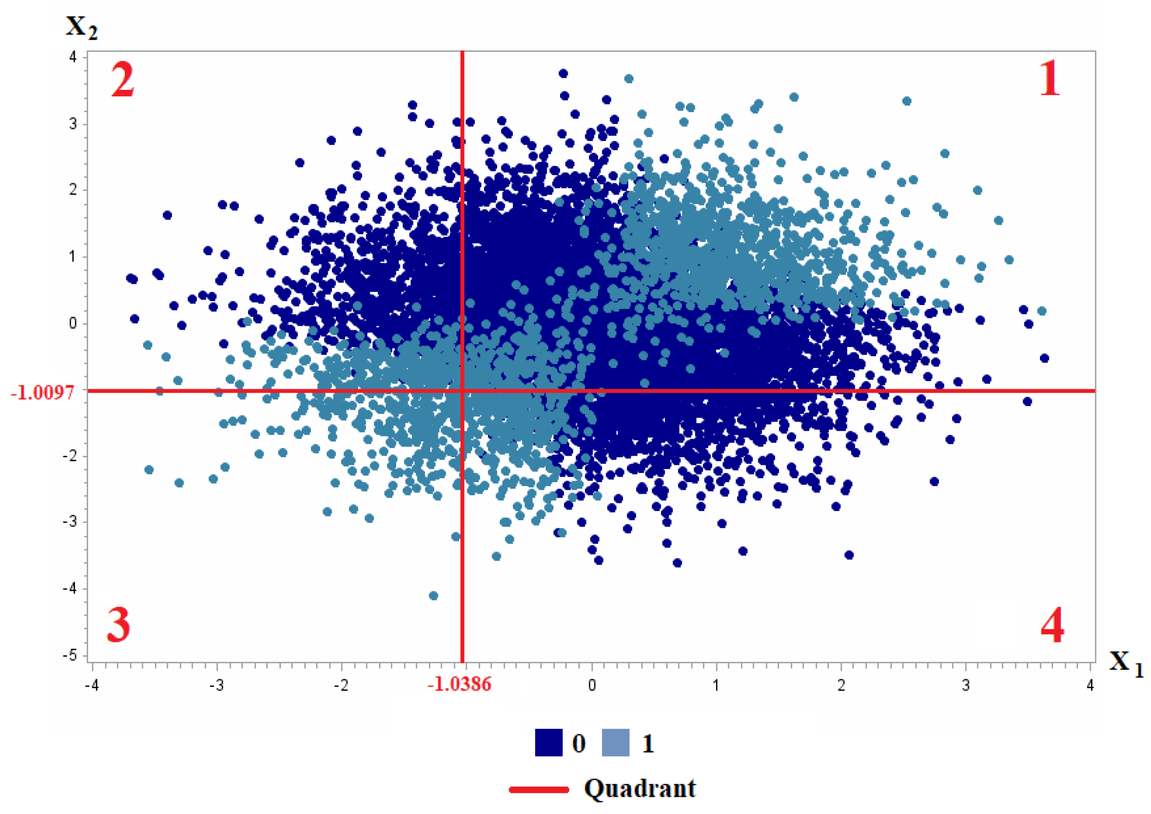
By generating values from such distribution, it is possible to obtain probabilities $P(Y=1)$. Simulated points $(x_1,x_2)$ are assigned to classes 1 or 0 depending on whether the corresponding probability lies above or below 0.5, respectively. Figure 1 shows the distribution of classes after 10000 simulations.

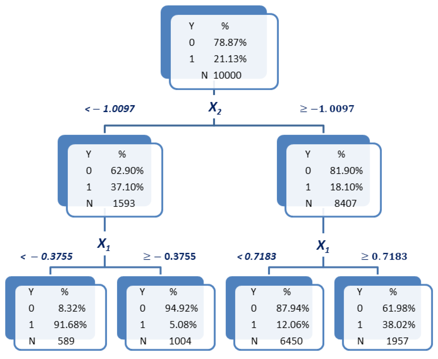
Let us now try to capture the observed interaction behaviour by means of (univariate) WOE variables. To this aim, WOE variables $W_{X_1}$ and $W_{X_2}$ are generated by discretizing variables $X_1$ and $X_2$ through classification trees based on the CHAID algorithm [22]. The result of this discretization process is shown in Figure 2. The values taken by the corresponding WOE variables, obtained by Equation (8), are presented below each tree leaf.

Then, the product variable $W_{X_1}·W_{X_2}$ is computed in order to provide the interaction term between variables $W_{X_1}$ and $W_{X_2}$.

Table 1. Frequency distribution of $W_{X_1}·W_{X_2}$ with respect to the four quadrants depicted in Figure 1.

	Quadrant
${\mathit{W}}_{{\mathit{X}}_{\mathbf{1}}}·{\mathit{W}}_{{\mathit{X}}_{\mathbf{2}}}$	1	2	3	4
$(-0.5164)·(-0.5279)$ = 0.2726	0	0	283	0
$(-1.4968)·(-0.5279)$ = 0.7902	0	0	0	1310
$(-0.5164)·(-1.5096)$ = 0.7796	0	1205	0	0
$(-1.4968)·(-1.5096)$ = 2.2596	7202	0	0	0

presents the frequency distribution of this product variable on the quadrants depicted in Figure 1, combining the cut-off points of the trees shown in Figure 2.

It is easily observed that the product $W_{X_1}·W_{X_2}$ takes a similar value in quadrants 2 and 4, but quite different values in quadrants 1 and 3. This is not adequate, since lower values should be associated to one of the classes and higher ones to the other. However, quadrants 1 and 3 are both mainly associated to class 1 and obtain the highest and lowest values for $W_{X_1}·W_{X_2}$, respectively. Consequently, the product $W_{X_1}·W_{X_2}$ does not seem to provide an adequate solution, at least in this case, for capturing the interaction between $X_1$ and $X_2$.

Alternately, fitting a single classification tree by using both variables $X_1$ and $X_2$ is considered. The obtained tree is shown in Figure 3. By looking at this tree, it is now observed that class 1 rates are higher in leaves 1 and 4 (counted from left to right), which by attending to the cut-off values imposed on both $X_1$ and $X_2$ can be observed to be associated with the previous quadrants 1 and 3. Conversely, class 1 rates are lower in leaves 2 and 3, associated with quadrants 2 and 4. Moreover, the cut-off values of $X_1$ indicate that the effect of this variable on class 1 rates varies depend on the values of $X_2$. When $X_2<-1.0097$ lower values of $X_1$ are associated with a greater class 1 rate. However, when $X_2\ge -1.0097$, the effect is the inverse: Greater values of $X_1$ are, in this case, associated with greater class 1 rates. Thus, this tree seems to capture the interaction behaviour between variables $X_1$ and $X_2$. Consequently, it would be sound to construct a (bivariate) WOE variable according to the leaves of this tree. Indeed, by applying Equation (13) in Section 3.2, the values of that WOE variable shown below the leaves of the tree in Figure 3 are obtained. Leaves 1 and 4 now receive lower values than leaves 2 and 3, and therefore this new WOE variable allows the reflection of the desired interaction effect. This is the intuition underlying the proposed bivariate WOE variables. The formal definition will be presented in Section 3.2.

Finally, let us remark that, regarding this example, another possibility would consist in first generating the product variable $Z=X_1·X_2$ and then constructing a WOE variable by discretization of Z through a (again univariate) classification tree. This approach, which is valid when $X_1$ and $X_2$ are continuous variables, is similarly adaptable to the case in which both variables are categorical. In this latter case, it would be enough to construct a categorical variable Z by crossing the categories of $X_1$ and $X_2$ and then to construct a (univariate) WOE variable after fitting the corresponding classification tree. However, when one of the variables, say $X_1$, is continuous and the other, $X_2$, is categorical, the discretization of $X_1·X_2$ would necessarily imply generating as many dummy variables as categories of $X_2$. This would make obtaining a unique WOE variable through Equation (8) impossible. The proposed methodology based on fitting classification trees to pairs of variables avoids this difficulty, since trees permits combining variables of any nature.

3.2. Generation of Bivariate WOE Variables

As illustrated in the motivating example of previous section, when the main effects in a logistic regression model are represented through univariate WOE variables $W_{X_i},i=1,\dots ,p$, the usual product interaction terms $W_{X_i}·W_{X_j},j\ne i,$ can fail to adequately capture the interaction behaviour between the corresponding original variables $X_i$ and $X_j$. This occurs mainly because univariate WOE transformations are carried out independently for each variable without taking into account the others. That is, the cut-off values obtained by each tree when generating each WOE variable are obtained by taking into account its direct relationship with the target variable Y. However, when another variable intervenes in this relationship, univariate trees cannot adapt and produces different cut-off points depending on the values of the other variable. Indeed, as explained in [18] in a statistical learning context, the depth of the decision trees assembled in a boosting model conditions the complexity of the model. When trees are at depth 1, the assembled models possess an additive nature with a single term that implies a single variable. However, greater levels of depth permit reflecting interactions between different variables if they alternate at these levels. This motivates our proposal of complementing univariate WOE-based logistic models with two-dimensional or bivariate WOE variables, obtained through fitting a classification tree to each pair of variables $X_i$ and $X_j$. Thus, the objective is to provide a general and widely applicable methodology enabling WOE-based logistic models to capture interactions effects.

Let us now focus on formally defining the construction of bivariate WOE variables. Given a pair of original input variables $X_i$ and $X_j,i,j=1,\dots ,p,i\ne j$, a classification tree is fitted to explain the response Y in terms of both $X_i$ and $X_j$. Let $C_{X_i\_X_j}$ denote the categorical variable for which its values $\{x_{ij,1},x_{ij,2},...,x_{ij,L_{X_{ij}}}\}$ identify each of the $L_{X_{ij}}$ leaves of the adjusted tree. From these categories, a WOE transformation can be applied to obtain what shall be called a bivariate WOE variable, which is to be denoted as $W_{X_i\_X_j}$. In this manner, in each leaf k of the tree (category $x_{ij,k}$), the transformed variable $W_{X_i\_X_j}$ is defined to take the value given by Equation (13).

$$W_{X_i\_X_j}\left(x_{ij,k}\right)=log{\displaystyle \frac{\widehat{p}(Y=1|C_{X_i\_X_j}=x_{ij,k})}{\widehat{p}(Y=0|C_{X_i\_X_j}=x_{ij,k})}}$$

(13)

Let us point out some remarks that are important to be taken into account:

• The fact that two variables are considered in the tree segmentation process does not guarantee that both will end up participating in it. For example, if $X_i$ and $X_j$ are two input variables, then it could be possible that only one of them appeared along the splitting process. Thus, in this case, the variable $W_{X_i\_X_j}$ reflecting the corresponding interaction effect is not considered to be defined, precisely because such interaction is not reflected in the tree.
• The subscript of variable $W_{X_i\_X_j}$ does not represent the order in which the variables participate in the segmentation process, but simply responds to a lexicographic order. This case is due to the fact that although the entry of $X_i$ could be forced in the first depth level and that of $X_j$ in the next, this would only reduce the predictive capability of the transformed variables included in the regression model. This circumstance is not adequate since, as mentioned in Section 2.1, the objective of using decision trees to perform the discretization of variables seeks to enhance the predictive capability of the obtained categories.
• Related to the previous point, at most only one interaction term is generated for each pair of variables. Thus, the maximum potential number of bivariate WOE variables to be included in the regression model is $\left(\genfrac{}{}{0pt}{}{p}{2}\right)$. In fact, the effective number will be lower if the tree generated for a pair $(X_i,X_j)$ does not include one of these variables.

Therefore, a distinction is made between two types of WOE variables:

• Univariate WOE variables with notation $W_{X_i}$ and generated through Equation (8).
  Let ${\overrightarrow{W}}_{uni}=(W_{X_1},W_{X_2},\dots ,W_{X_p})$ denote the vector of univariate WOE variables obtained from the original variables;
• Bivariate WOE variables denoted $W_{X_i\_X_j}$ and generated through Equation (13).
  Let ${\overrightarrow{W}}_{bi}=(W_{X_1\_X_2},W_{X_1\_X_3},\dots ,W_{X_{p-1}\_X_p})$ denote the vector of bivariate WOE variables obtained from pairs of original variables.

Thus, in principle, the fit of a full logistic regression model using the univariate WOE variables ${\overrightarrow{W}}_{uni}$ associated with all available inputs, as well as the bivariate WOE transforms ${\overrightarrow{W}}_{bi}$ corresponding to all possible pairs of such inputs can be considered. This would result in the model given by Equation (14).

$$logit\left(\pi ({\overrightarrow{W}}_{uni},{\overrightarrow{W}}_{bi})\right)={\beta }_0+{\beta }_1·W_{X_1}+...+{\beta }_p·W_{X_p}+\sum _{i=1}^p\sum _{\begin{array}{c}j=1\\ j\ne i\end{array}}^p{\beta }_{ij}·W_{X_i\_X_j}$$

(14)

Similarly to what was discussed at the end of Section 2.3, neither the coefficient ${\beta }_{ij}$ of the bivariate WOE variable $W_{X_i\_X_j}$ nor its odds ratio allow an interpretation of the interaction effect between the original variables $X_i$ and $X_j$ on the response. Rather, this interpretation is provided by the classification tree model associated with the definition of $W_{X_i\_X_j}$, from which it is possible to assess the different cut-off values obtained for a variable, say $X_j$, given the previous cut-off points for $X_i$, as well as to compare them with the cut-off values produced in the corresponding univariate trees fitted in the construction of both $W_{X_i}$ and $W_{X_j}$. Furthermore, it is possible to easily adapt the score points transformation in Equation (11) in order to provide an explanation of the relative effect of variable $W_{X_i\_X_j}$ on the loan decision regarding a given client, as shown in Equation (15):

$$SCOR{E}_{X_i\_X_j}\left(x_{ij}\right)=(-W_{X_i\_X_j}\left(x_{ij}\right)·{\beta }_{ij}+{\beta }_0/m)\ast factor+offset/m$$

(15)

where

• ${\beta }_{ij}$ is the regression coefficient associated to variable $W_{X_i\_X_j}$;
• ${\beta }_0$ is the intercept or constant term of the regression model;
• m is the total number of variables effectively included in the regression model in Equation (14);
• $factor$ and $offset$ are scale parameters that allow the analyst to control the range of the score function as well as the needed variation in the odds ratio for a given increase in points.

Let us now discuss some practical aspects regarding the configuration of the growing process of the classification trees to be employed in the construction of both univariate and bivariate WOE variables:

• It is important to notice the interdependence between the number of obtained tree leaves, on the one hand, and the interpretability and predictive capability of the resulting tree models, on the other hand. Typically, allowing more tree leaves will result in an enhanced predictive capability of the resulting WOE variables, at least until overfitting issues appear. However, a tree with many leaves will usually also be more difficult to interpret.
• The interpretability of univariate WOE variables used is to be associated with a certain monotonicity of the default rates in relation to the categories obtained for the original input variable. Such monotonicity is more difficult to achieve as the number of categories increases. Obviously, monotonicity of the default rates is not a problem when only two tree leaves or categories are considered. However, this quantity used is too small for adequately representing the variability of the input and tends to provide a poor predictive capability. In this sense, it has been considered that a maximum of four leaves may provide a good trade-off between interpretability and predictive capability of the resulting univariate WOE variables. In future works, this issue will be analyzed.
• In the case of bivariate WOE variables, interpretability is not as dependent on monotonicity since they are devised to capture interaction behaviours that manifest through variations in the trends of the univariate WOE variables. However, in this case, two is the minimum depth required in binary branching trees in order to allow reflecting an interaction between two variables, although the associated predictive capability may be rather poor. On the other extreme, allowing more than 16 categories (those that would result from crossing two variables with four categories each) can result in model that is too complex to interpret.
• How can the number of obtained leaves be controlled in order to remain between the discussed ranges? In the case of univariate WOE variables, the only two options would be using either a depth-2 tree with binary branching or a depth-1 tree with up to four branches. Although binary branching is most well-known and extended, depth-1 trees with 4-ary branching provide a more convenient option in this case since they tend to provide more leaves than depth-2 trees with binary branching. Precisely for this reason, in the case of bivariate WOE variables, binary-branching trees with a depth-level between two and four are instead preferred, as a slightly lower number of leaves may favour interpretability of the interaction behaviour.
• CHAID-like classification trees [22] can be used to establish significance levels and test for the statistical significance of each tree leaf. This may provide more robust categories with an enhanced predictive behaviour in comparison to other methodologies, such as CART-like classification trees [23]. However, precisely because of their more demanding branching process, CHAID trees tend to provide less leaves than CART trees, and they can even avoid the discretization of some inputs. In this sense, when a variable selection procedure (e.g., stepwise variable selection) is applied after the construction of WOE variables, CART-like trees may be preferable to CHAID ones. This happens since the former guarantees the discretization of the original inputs, and although the predictive capability of some resulting WOE variables may be comparatively lower, the variable selection procedure would discard them during the model building process.
• Both in the case of univariate and bivariate WOE variables and independently of using either CHAID or CART trees, pruning the resulting trees by using a validation sample before actually computing the WOE transformation may allow the improvement of the actual predictive capability of the resulting WOE variables, as well as the enhancement of its interpretability.

As just mentioned, once WOE variables have been constructed it may be worth applying a variable selection procedure in order to enhance interpretability and avoid overfitting by obtaining a model with lower complexity to that of the full model in Equation (14). In particular, some variants of the stepwise procedure can further enhance interpretability when working with WOE variables (see [24]). Moreover, when a validation sample is available in addition to a training one, the sequence of models provided by the application of the variable selection procedure on the training sample can be ranked in terms of a performance criteria obtained on the validation sample. In this manner, the model finally selected would be the model in the sequence with best performance on the validation sample.

Finally, let us summarize the main ideas supporting the use of the proposed bivariate WOE variables methodology:

• In the definition of $W_{X_i\_X_j}$, the interaction between the variables $X_i$ and $X_j$ from which it is generated is implicit. Therefore, bivariate WOE variables allow addressing the main criticism regarding the use of (univariate) WOE variables that refers to their incapability to reflect interaction effects, as univariate classification trees are unable to produce different cut-off points depending on the values of other variables.
• WOE variables, as explained in Section 2.3, allow retaining most of the advantages associated with the discretization of input variables in the context of logistic regression (outliers and missing values and non-monotonous effects) while avoiding its main drawbacks (the potentially huge number of dummy variables to be considered and the associated dilemma regarding the inclusion of non-significant effects). This also applies to bivariate WOE variables since bivariate trees behave similarly to univariate ones in this respect (let us remark that the term bivariate tree is used to emphasize the presence of two explanatory variables instead of a single one). Moreover, bivariate WOE variables contribute to a potentially greater reduction than univariate ones in the number of variables to be considered since they allow concentrating the information of up to $\left(\genfrac{}{}{0pt}{}{p}{2}\right)·{(L-1)}^2$ crosses of dummy variables for interaction terms into just $\left(\genfrac{}{}{0pt}{}{p}{2}\right)$ bivariate WOE variables (see also Section 2.2).
• The construction steps of bivariate WOE variables do not depend on the nature or typology of the two original input variables being combined. A bivariate classification tree provides the basis for applying Equation (13) independently of whether the original variables are both continuous, both categorical or one continuous and the other categorical. This fact does not hold when trying to model interactions through univariate WOE transforms of the product or combination of the original variables since there is no way to produce a single interaction term in case one of the original variables is continuous and the other is categorical. In this sense, bivariate WOE variables provide a more general methodology to deal with interactions than univariate WOE transforms of usual interaction terms.
• Bivariate WOE variables are constructed in such a way that only existing interactions are reflected. In this sense, notice that a cross $W_{X_i}·W_{X_j}$ between univariate WOE variables may not be significant or possess insufficient case support in order to be generalizable. However, each value of the variable $W_{X_i\_X_j}$ is supported by a leaf of a classification tree for which its minimum support can be prespecified in order to guarantee some level of generalizability. Furthermore, CHAID-like classification trees can be used whenever statistical significance of the discretized categories is required.
• Let us remark that variables $W_{X_i\_Xj}$ arise from making $X_i$ and $X_j$ interact, but they are not the result of the interaction of $W_{X_i}$ and $W_{X_j}$. This observation is important since, as $W_{X_i\_X_j}\ne W_{X_i}·W_{X_j}$, the fulfillment of the hierarchical principle (see Section 2.2) does not apply to a stepwise variable selection process in the context of the model in Equation (14). This circumstance provides more flexibility to the proposed methodology.
• The interaction behaviour associated to variables $W_{X_i\_Xj}$ can be interpreted through the bivariate trees associated to their construction, and their effect on loan decisions can be explained through score points transformations.

3.3. Illustrative Example

The objective of this section is to briefly illustrate how bivariate WOE variables allow capturing interaction patterns between variables, as well as the potential ease they provide for the interpretation of such interaction effects. To this aim, the $CS\_ACCEPTS$ dataset, for which its description can be observed in Appendix A, will be used. In this manner, this section complements the motivating example in Section 3.1, showing that the alleged features of bivariate WOE variables can indeed be useful on real data. Particularly in the first part of this example, the focus will be on variables $AGE$ (age in years of a client asking for credit) and $CHILDREN$ (number of children of a client) of the $CS\_ACCEPTS$ dataset. As it is well-known for credit scoring analysts, both variables usually present a meaningful interaction, namely the effect of having children on loan default probability is dependent on the age of the clients.

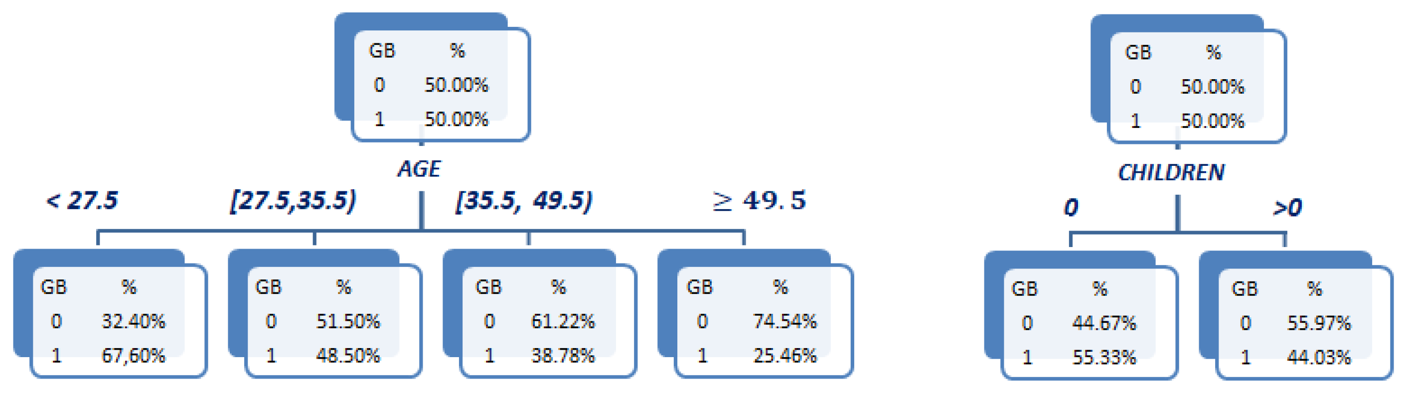
To begin, a pair of CART classification trees are fitted to explain the target variable GB (=1 ($Bad$), = 0 ($Good$)) according to $AGE$ and $CHILDREN$, respectively, in order to obtain the univariate WOE variables $W_{AGE}$ and $W_{CHILDREN}$.

As recommended in the last section, a depth-1, 4-ary branching configuration is used in the case of $AGE$. The resulting tree is shown in Figure 4 (left). Notice the (decreasing) monotonicity of the default rates as $AGE$ increases that allows a clear interpretation of the effect of this variable on the default probability: The higher the age of a client, the lower the probability of defaulting. The values of the corresponding $W_{AGE}$ variable are given in

Table 2. Values obtained for $W_{AGE}$ from the tree depicted in Figure 4 (left).

$\mathit{LEAF}$	$\mathit{AGE}$	${\mathit{W}}_{\mathit{AGE}}$
1	$(-\infty ,27.5)$	$0.735396727$
2	$[27.5,35.5)$	$0.0598981416$
3	$[35.5,49.5)$	$0.4566512156$
4	$[49.5,\infty )$	$1.0742208355$

, showing also the mentioned monotone behaviour. For illustrative purposes, a depth-1 tree with just binary branching is used for $CHILDREN$. This allows a simple monotone pattern to also arise in this case: Clients with children have a lower default probability, as can be observed in the tree at Figure 4 (right). The obtained values of $W_{CHILDREN}$ are provided in

Table 3. Values obtained for $W_{CHILDREN}$ from the tree depicted in Figure 4 (right).

$\mathit{LEAF}$	$\mathit{CHILDREN}$	${\mathit{W}}_{\mathit{CHILDREN}}$
1	0	$-0.214062899$
2	$(0,\infty )$	$0.240014873$

.

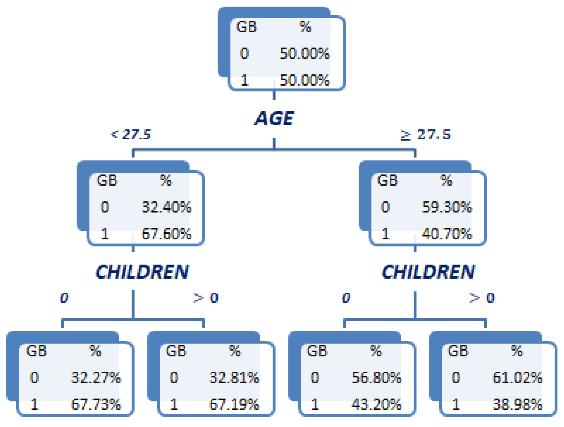
Now, a third tree in which both $AGE$ and $CHILDREN$ simultaneously participate is fitted to generate the bivariate WOE variable $W_{AGE\_CHILDREN}$. This binary branching depth-2 tree is shown in Figure 5. The cut-off values in this tree have been introduced manually in order to reproduce the analyst intuition that the main difference in the effect of having children is between young (i.e., $AGE<27.5$) and not-young ($AGE\ge 27.5$) clients. The resulting tree captures this interaction pattern: the effect of having children on default probability is almost nonexistent in the case of young clients (67.73% for clients without children vs. 67.19% for clients with children), while it is quite more significant for not-young clients (43.20% vs. 38.98%; a 4% reduction in absolute terms). The bivariate WOE variable $W_{AGE\_CHILDREN}$ for which its values are provided in

Table 4. Values obtained for $W_{AGE\_CHILDREN}$ from the tree depicted in Figure 5.

$\mathit{LEAF}$	$\mathit{AGE}$	$\mathit{CHILDREN}$	${\mathit{W}}_{\mathit{AGE}\_\mathit{CHILDREN}}$
1	$(-\infty ,27.5)$	0	$-0.741372533$
2	$(-\infty ,27.5)$	$(0,\infty )$	$-0.716957829$
3	$[27.5,\infty )$	0	$0.2738586439$
4	$[27.5,\infty )$	$(0,\infty )$	$0.447963401$

adequately reflects this interaction effect, taking quite similar values in the first two leaves associated to young clients, while being noticeably different in the last two leaves associated with not-young clients. Notice that the tree in Figure 5 could be prunned by the branch associated with the younger clients. However, it has been left unprunned for the illustrative purposes of this example.

Let us now introduce a second example focusing on variables $CARDS$ (type of credit card owned by a client) and $CASH$ (loan requested cash in US$) of the same $CS\_ACCEPTS$ dataset. Notice that $CARDS$ is a nominal variable, while $CASH$ is a continuous one. This example will then allow the illustration of the mentioned capability of the proposed bivariate WOE variables methodology in order to deal with this casuistic, which is otherwise difficult to deal with without introducing as many dummy variables as categories of the nominal variable (minus one).

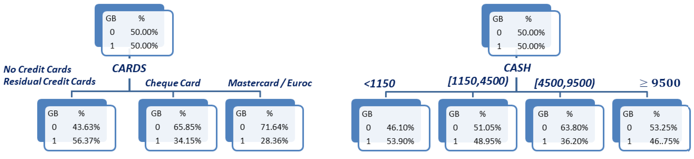
As before, the first step consists of fitting a pair of depth-1, 4-ary branching CART trees explains the response $GB$ in terms of $CARDS$ and $CASH$, respectively. The resulting trees are shown in Figure 6. Notice that, although a 4-ary branching tree was requested, the tree for $CARDS$ only has three leaves. This is due to the very reduced support of the Residual Credit Cards category (which includes Visa and American Express, among others) that holds for just 10 observations or clients in the $CS\_ACCEPTS$ dataset. Since a 1% support threshold was required to create a leaf, this category was merged in the tree with No Credit Cards. Regarding the tree for $CASH$, the first 3 categories present a (decreasing) monotone behaviour of the default rates, which is broken at the last category containing the highest loans ($CASH\ge 9500$). Although this pattern may seem counter-intuitive at first sight, it actually is not so: Lowest loans ($CASH<1150$) are typically asked only by low-income clients, which explains the relatively high default rate at this category. Higher loans ($CASH\in [1150,4500)$ or $CASH\in [4500,9500)$) tend to be only granted to relatively middle-to-high-income clients, thus explaining the decreasing pattern of default rates. However, the highest loan category contains considerably high loans ($max\left(CASH\right)=100,000$), which may be defaulted even by high-income clients. This explains why the default rate rises at this category. The values obtained for the corresponding WOE variables $W_{CARDS}$ and $W_{CASH}$ are provided in

Table 5. Values obtained for $W_{CARDS}$ from the tree depicted in Figure 6 (left).

$\mathit{LEAF}$	$\mathit{VALUES}$	${\mathit{W}}_{\mathit{CARDS}}$
1	$NoCreditCards/Residual$	$-0.256378923$
2	$ChequeCard$	$0.6566397642$
3	$Mastercard/Euroc$	$0.9267620317$

and

Table 6. Values obtained for $W_{CASH}$ from the tree depicted in Figure 6 (right).

$\mathit{LEAF}$	$\mathit{VALUES}$	${\mathit{W}}_{\mathit{CASH}}$
1	$(-\infty ,1150)$	$-0.1564247$
2	$[1150,4500)$	$0.0418972109$
3	$[4500,9500)$	$0.5668534552$
4	$[9500,\infty )$	$0.1300531282$

, respectively.

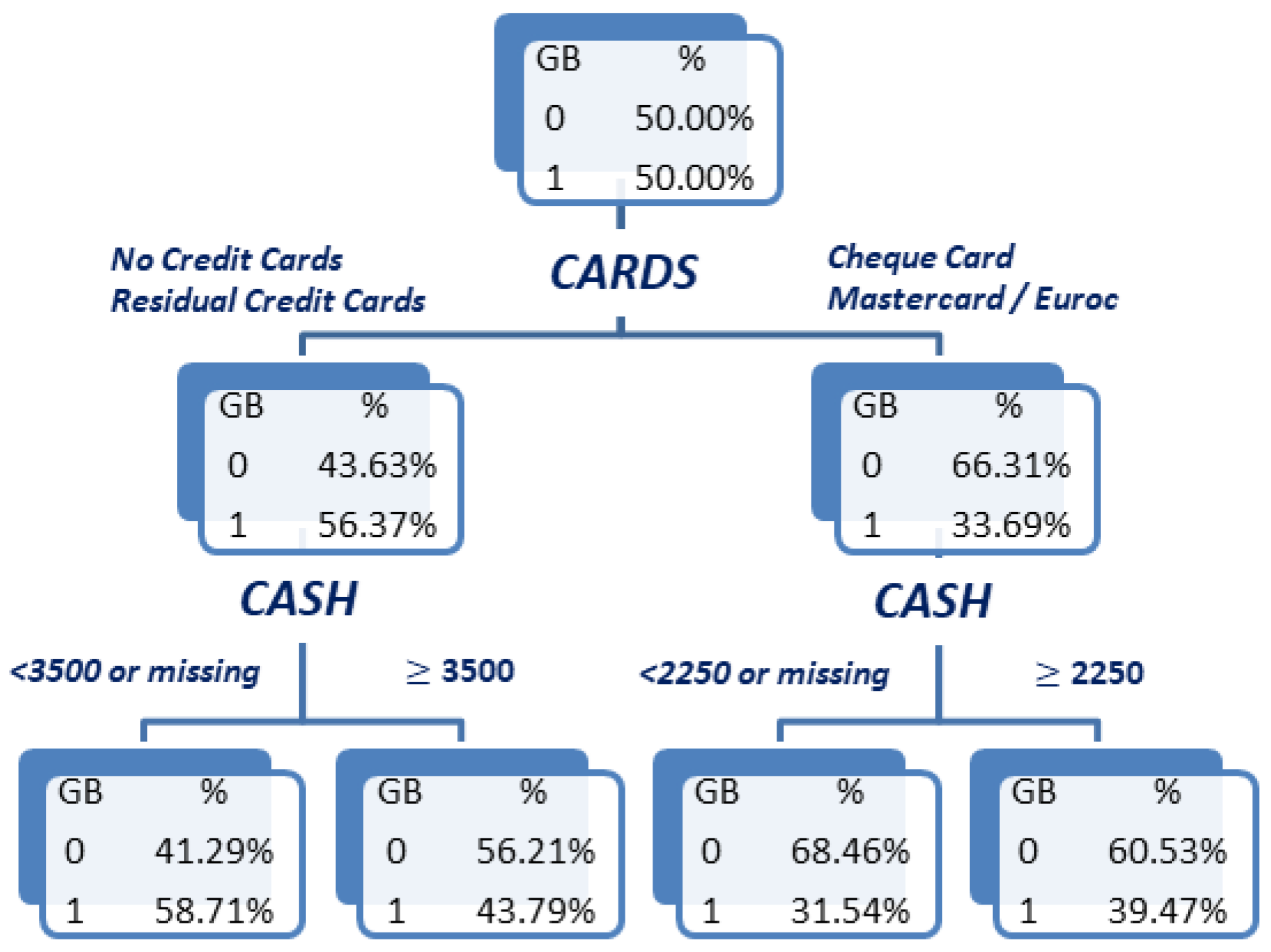
Now, a binary branching, depth-2 CART tree is fitted using both $CARDS$ and $CASH$ to obtain the bivariate WOE $W_{CARDS\_CASH}$ variable (see Figure 7). By looking at the leaves of this tree, a variation in the effect of $CASH$ on default probability depending on the credit cards owned by clients can be observed: When the client possesses either no credit card or a residual card, higher loans ($CASH\ge 3500$) are associated with a lower default rate than lower loans. However, when the client possesses either a Cheque Card or a Mastercard/Eurocard, higher loans (now $CASH\ge 2250$) are instead associated with a higher default probability than lower loans. The bivariate WOE variable $W_{CARDS\_CASH}$ for which its values are provided in

Table 7. Values obtained for $W_{CARDS\_CASH}$ from the tree depicted in Figure 7.

$\mathit{LEAF}$	$\mathit{CARDS}$	$\mathit{CASH}$	${\mathit{W}}_{\mathit{CARDS}\_\mathit{CASH}}$
1	$NoCreditCards/Residual$	$(-\infty ,3500)$	$0.7747746746$
2	$NoCreditCards/Residual$	$[3500,\infty )$	$0.4274440148$
3	$Mastercard/Euroc$	$(-\infty ,2250)$	$-0.352137368$
4	$Mastercard/Euroc$	$[2250,\infty )$	$0.2498117984$

reflect this interaction pattern, taking a lower value in leaf one than in leaf two, while instead taking a greater value in leaf four than in leaf three.

In addition to this variation in the effect of $CASH$ for different credit cards, another fact to emphasise is that, in the tree in Figure 7, the cut-off value for $CASH$ also varies depending on $CARDS$: In the left branch for $CARDS$, the cut-off for $CASH$ is 3500, while in the right branch it is 2250. Therefore, the interaction between a pair of variables may not only be reflected through changes in the trend of the default probability as the second variable to enter the tree varies but also through variations in the cut-off values obtained for the second variable that separates the categories in which such variations in trend may occur. Obviously, this kind of interaction effect cannot be reflected through products of univariate WOE variables, since the cut-off values obtained in the univariate trees will determine the joint categories obtained from crossing the univariate variables. In this sense, notice also that the cut-off values for $CASH$ obtained in the bivariate tree in Figure 7 do not coincide with those obtained for the same variable in the univariate tree in Figure 6 (right). These observations further illustrate the flexibility provided by bivariate WOE variables to capture different aspects of the interaction between a pair of variables.

4. Computational Study

This section is devoted to presenting a computational experiment carried out in order to assess the predictive behaviour of the proposed methodology in the context of WOE-based logistic regression models for credit scoring. To this aim, Section 4.1 details the experimental setting of this computational study: methods to be compared, datasets to be used, division of the data, evaluation metric, etc. Next, Section 4.2 presents and discuss the obtained results, providing statistical tests to rigorously compare the performance of the methods being assessed.

4.1. Experimental Framework

A set of WOE-based logistic regression models will be applied to different datasets in order to assess the potential benefits of adding bivariate WOE variables to capture interactions between variables. In this sense, the baseline or reference method will be given by logistic regression models fitted through a stepwise variable selection procedure by using only univariate WOE variables without any interaction term. A first variation of this reference will be provided by the inclusion of interaction terms given by the product of univariate WOE variables, either fulfilling or not fulfilling the hierarchical principle. Finally, the reference models will also be modified instead by adding bivariate WOE variables created by using classification trees with different depth levels.

Note that stepwise selection has been used instead of the well-known Information Value for feature selection based on WOE variables definition [14] because it must be observed that the selection method based on the Information Value criteria does not take into account possible interactions between variables. So for example, we can consider a regressor which is only related with the dependent variable through the interaction with another regressor, but not directly related with the target. In this case, Information Value criteria would not select the variable but stepwise method would do it in the case that the other regressor would have been previously included in the model.

Specifically, the following kinds of logistic regression models will be used:

• No Int.: Models using univariate WOE variables as main effects but without interaction terms between these univariate WOE variables. This constitutes the baseline or reference method of the study.
• Int.(HP): Interaction terms given by products of univariate WOE variables are allowed to enter the previous reference model, forcing the hierarchical principle to always be fulfilled. That is, the interaction term $W_{X_i}·W_{X_j}$ can only be included in a model if both $W_{X_i}$ and $W_{X_j}$ are already included.
• Int.(NHP): The same configuration as Int.(HP) but without forcing the hierarchical principle to be fulfilled. The elimination of this restriction seeks to maximize the predictive capacity of the models.
• BiWOE2: Bivariate WOE variables created through binary branching, depth-2 trees are allowed to be included in baseline No Int. models to capture interactions between variables. In this manner, bivariate WOE variables replace the product interaction terms used in configurations Int.(HP) and Int.(NHP).
• BiWOE4: The same configuration as BiWOE2 but by using depth-4 trees to create bivariate WOE variables.

For all five methods, some considerations must be made regarding the configuration of the classification trees used to create both univariate and bivariate WOE variables from the original inputs:

• For univariate WOE variables, all inputs are discretized in a maximum of four categories. In order to achieve this, either 4-ary branching, depth-1 trees (Tree = (Depth1)) or binary branching, depth-2 trees (Tree = (Depth2)) have been used. Both kinds of trees are applied for obtaining the univariate WOE variables in each of the above five methods to assess whether the tree typology influences their predictive capability. A priori, as mentioned in Section 3.2, the former trees are more likely to reach the maximum of four categories.
• Bivariate WOE variables are created for each pair of original inputs. As just mentioned, the effect of depth-2 and depth-4 trees is compared, in both cases with binary branching. As explained in Section 3.2, the former trees are in principle more adapted to achieve easily interpretable models, while the last trees would provide a greater predictive capability. Thus, it should be noted that depth-4 trees allow obtaining up to 16 categories, which is the same as the number of different WOE values obtained as a product of two univariate WOE variables with four categories each.
• For both univariate and bivariate WOE variables, two different algorithms have been considered to grow the trees:

  –

  CHAID trees (Tree=CHAID): A significance level of 0.2 (SAS Enterprise Miner default value) is established for the Chi-square tests involved in the segmentation. The tree pruning process is carried out attending to the minimization of the misclassification rate of the model (on a validation sample);

  –

  CART trees (Tree=CART): The Gini index is used for both segmentation and pruning.

• In addition to the stopping criteria associated with the significance level (for CHAID trees) and the depth level of the trees, an additional support criterion has been established through the minimum number of observations any leaf must contain, established at 1% of the observations in the training sample.

The study has been carried out on 12 well-known reference datasets within the scope of credit scoring. The main details of these 12 datasets are provided in

Table 8. Main details of the 12 datasets employed in the computational study: name of the dataset, number of inputs (number of numeric/categorical variables), number of observations, presence of missing values, and ratio between default and non-default observations.

Dataset	Inputs	Patterns	Missings	Ratio
AUSTRALIAN	14 (6/8)	690	NO	44.49%
CREDIT_CARD	9 (4/5)	1319	NO	22.44%
CS_ACCEPTS	26 (13/13)	3000	YES	50.00%
GERMAN_CREDIT	20 (3/17)	1000	NO	30.00%
GIVE_ME_SOME_CREDIT	10 (5/5)	150,000	YES	6.68%
HMEQ	12 (7/5)	5960	YES	19.95%
JAPAN	15 (6/9)	690	YES	44.49%
LOAN_DATA	14 (9/5)	1225	NO	26.37%
MORTGAGE	18 (4/14)	41,747	NO	36.31%
PAKDD	52 (7/45)	50,000	YES	26.08%
POLISH	18 (18)	43,405	YES	4.82%
TAIWAN	23 (14/9)	30,000	NO	22.12%

. The datasets and their description are accessed on 29 June 2021 and available at https://github.com/JLZml/Credit-Scoring-Data-Sets. Appendix B provides some further considerations regarding the definition of the target variable and the exclusion of some inputs from these datasets.

In order to fit models and to assess their performance, each dataset has been randomly partitioned into three samples by using stratified sampling in order to obtain similar proportions for the classes of the target variable (the percentage distribution responds to the default configuration of SAS Enterprise Miner):

• A training sample containing 40% of the dataset observations, which is first used for growing both univariate and bivariate trees, as well as to compute the values of the WOE variables after the trees are pruned. Later, the same training sample is used to apply stepwise variable selection in order to create a sequence of models for each of the five applied methods.
• A validation sample containing 30% of the dataset observations, which is first used to prune the trees grown with the training sample and later to select a model from the stepwise sequence of models created with the training sample.
• A test sample with 30% of the dataset observations, which is only used to compute a performance metric for the selected model (for this dataset) of each method.

Therefore, in each of the 12 datasets, for each of the above described five methods and for each combination of tree depth levels (for univariate WOE variables) and tree-growing algorithms, the following steps are applied:

• Grow both univariate and bivariate trees using the training sample;
• Prune both kinds of trees using the validation sample;
• Compute both univariate and bivariate WOE variables on the corresponding pruned trees by using the training sample;
• Apply standard stepwise variable selection by using the training sample, thus obtaining a sequence of models;
• Select the model in the sequence with the best performance on the validation sample;
• Assess the performance of the selected model on the test sample.

The performance metric used for both model selection (step 5) and final model evaluation (step 6) is the area under the ROC curve, that is, the AUC metric. This metric has been chosen since its application in the credit scoring field is rather usual due to the typically unbalanced nature of the datasets, which result in trying to obtain models that maximize AUC instead of just classification accuracy [25].

4.2. Results

In this section, the results obtained after applying the experimental setting described in the previous section are presented and discussed. The discretization process and the regression models have been adjusted by using the Credit Scoring module of the Enterprise Miner tool of the SAS software. This solution has been chosen since the functions that this module has implemented are especially oriented to the treatment of Credit Scoring problems. On the other hand, the comparison of results has been carried out by using the functions friedman.test and wilcox.test of the package stats of the R software [26], since a function has not been found that would allow this comparison to be made in the specified SAS module.

Table 9. AUC test performances by dataset for each combination of tree growing algorithm, depth of the trees, and method.

Tree	Method	AUSTRA	CCARDD	CSACPT	GERMAN	GMSC	HMEQ	JAPAN	LOANDA	MORTGG	PAKDD	POLISH	TAIWAN
CHAID (Depth1)	No Int.	0.9036	0.6930	0.7108	0.6238	0.6564	0.8907	0.9402	0.5881	0.8156	0.6058	—	0.7669
	Int.(HP)	0.8870	0.6930	0.7108	0.6238	0.6564	0.8907	0.9402	0.5881	0.8178	0.6000	—	0.7669
	Int.(NHP)	0.8899	0.6930	0.7108	0.6238	0.6564	0.8963	0.9401	0.5881	0.8179	0.602	—	0.7659
	BiWOE2	0.9197	0.7818	0.7244	0.7319	0.6562	0.8979	0.9309	0.5881	0.8241	0.6006	—	0.7654
	BiWOE4	0.8939	0.7980	0.7149	0.7319	0.7784	0.9082	0.9309	0.5892	0.8237	0.6085	0.7478	0.7644
CHAID (Depth2)	No Int.	0.8975	0.6453	0.7052	—	0.6564	0.8761	0.9411	0.5881	0.7973	0.6030	—	0.7584
	Int.(HP)	0.8913	0.6453	0.7052	—	0.6564	0.8761	0.9411	0.5881	0.7936	0.5905	—	0.7588
	Int.(NHP)	0.8909	0.6453	0.6978	—	0.6564	0.8745	0.9373	0.5881	0.7966	0.6032	—	0.7632
	BiWOE2	0.9197	0.7330	0.7167	0.7297	0.6562	0.8891	0.9309	0.5881	0.8166	0.5998	—	0.7584
	BiWOE4	0.8967	0.7561	0.7149	0.7297	0.7784	0.9909	0.9309	0.5892	0.8365	0.5967	0.7478	0.7566
CART (Depth1)	No Int.	0.8817	0.7428	0.7148	0.7473	0.8502	0.9045	0.9402	0.5817	0.8308	0.6124	0.8050	0.7705
	Int.(HP)	0.8820	0.7428	0.7148	0.7448	0.8497	0.9035	0.9399	0.5817	0.8333	0.6144	0.8038	0.7714
	Int.(NHP)	0.8558	0.7486	0.7163	0.7438	0.8511	0.9054	0.9218	0.5603	0.8355	0.6126	0.8327	0.7703
	BiWOE2	0.9013	0.8011	0.7245	0.7548	0.8569	0.9057	0.9318	0.5906	0.8373	0.6163	0.8614	0.7713
	BiWOE4	0.8918	0.8021	0.7258	0.7444	0.8614	0.9116	0.9525	0.5865	0.8493	0.6218	0.8977	0.7737
CART (Depth2)	No Int.	0.8965	0.7634	0.7187	0.7015	0.8587	0.9058	0.9470	0.5817	0.8358	0.6152	0.8346	0.7677
	Int.(HP)	0.8917	0.7634	0.7185	0.7015	0.8584	0.9024	0.9417	0.5817	0.8408	0.6157	0.8359	0.7658
	Int.(NHP)	0.8917	0.7624	0.7195	0.7132	0.8608	0.9089	0.9339	0.5652	0.8407	0.6172	0.8366	0.7682
	BiWOE2	0.9073	0.8088	0.7264	0.7458	0.8605	0.9058	0.9318	0.6091	0.8358	0.6197	0.8579	0.7665
	BiWOE4	0.8918	0.8025	0.7236	0.7444	0.8614	0.9116	0.9525	0.5865	0.8489	0.6203	0.8956	0.7737

shows the test AUC performances of the five compared methods in each dataset for each combination of tree depth levels and tree growing algorithms. Within each table cell, the best performance among the five methods is highlighted in bold type. Moreover, the best performance for each dataset is underlined. In Appendix C, a more detailed description of the models resulting from the application of the stepwise selection procedure on the $CS\_ACCEPTS$ datasets can be found.

Notice that there are 11 cases for which no AUC result is shown. This occurs because no WOE variables were generated during the discretization process. Consequently, there were no variables to include in the regression model. This can happen with the CHAID algorithm when the chi-squared tests carried out to determine if there is a dependence relationship between the variable to be categorized and the response is above the pre-established significance level. This circumstance can also occur if, once the segmentation is completed, the pruning process leaves the tree reduced to the root node. In any case, it can be observed that this situation did not occur for any of the results of the method BiWOE4; that is, the bivariate WOE variables are obtained through depth-4 trees, which is a point in favor for using this methodology in comparison with the rest.

In order to rigorously compare the performance of the five methods, a statistical analysis using non-parametric tests following the recommendations made in [27] was performed. It is a set of simple, safe and robust non-parametric tests [28,29,30] where objective is to evaluate if there are significant differences between the median performances of the different methods. For multiple comparisons, the Friedman test [31] is used and the Wilcoxon Signed-Ranks test [32] adjusted with the Holm method [33] is used for pairwise comparisons.

In order to carry out multiple comparisons, it is necessary to first check if the results obtained by all methods present significant differences (Friedman test). If that is the case, pairwise differences can then be searched by using a post hoc test to compare the control method (in this case, BiWOE4) with the remaining ones (Holm test). The level of significance contemplated to carry out the analysis has been $0.05$.

The results of the multiple comparisons between the different methods as well as the pairwise comparisons are shown in

Table 10. Results of non-parametric tests. Holm test p-values of the pairwise comparisons (for each combination of tree growing algorithm and depth) are given at the four middle rows. Friedman test p-values for multiple comparisons are given in the last row.

Comparison	CHAID1	CHAID2	CART1	CART2
BiWOE4 vs. No Int	0.664	0.931	0.026	0.034
BiWOE4 vs. Int.(HP)	0.294	0.528	0.026	0.025
BiWOE4 vs. Int.(NHP)	0.294	0.884	0.025	0.025
BiWOE4 vs. BiWOE2	0.999	0.954	0.679	0.999
Friedman-test	0.075	0.373	<0.001	<0.001

. In the last row, it is observed that no significant differences for CHAID trees were found between the different methods ($p=0.075$ and $p=0.373$, respectively, for depth-1 and depth-2 trees). However, when analyzing the results for the CART trees, significant differences were found since $p<0.001$ in both cases. When studying pairwise comparisons for the methods using CART trees, the $BiWOE4$ method was found to be superior to the $NoInt.$ method ($p=0.026$ and $p=0.034$). The former also shows superiority when compared to $Int.\left(HP\right)$ and $Int.\left(NHP\right)$ ($p=0.026$ and $p=0.025$). Finally, no statistically significant differences were found between the BiWOE2 and BiWOE4 methods when using CART trees ($p=0.679$ and $p=0.999$).

5. Conclusions

An extension of the WOE-based methodology usually applied for credit scoring purposes has been presented in this work. The main aims of this extension are as follows: (1) addressing the lack of adaptation of the standard WOE-based approach to deal with interacting variables; and, related to the previous point, (2) enhancing the predictive capability of the WOE-based methodology while simultaneously safeguarding its interpretability and, particularly, its main interpretability tool, that is, balance scorecards.

The core of the proposed extension resides at the discretization process intended to transform the original inputs into explanatory WOE variables to be introduced in a logistic regression model. It has been shown that by simultaneously discretizing each pair of inputs through a single classification tree, it is possible to obtain a new kind of WOE variable that allows reflecting the interaction behaviour between such pair of inputs. The tree model underlying the construction of these variables allows for an easy interpretation of the interaction effects involved. Furthermore, it is straightforward to extend the scorecards methodology to provide explainability tools for the proposed extended methodology. Moreover, the proposed extension provides a general and widely and easily applicable methodology to reflect interaction effects in a WOE-based logistic regression model since it can be applied to any pair of inputs independent of their (continuous or categorical) nature and avoids both the usual problems derived from the generation of (possibly a lot of) dummy variables and the dilemmas regarding their statistical significance.

Moreover, the computational study presented in this work shows that the proposed extension allows a statistically significant improvement on the predictive capability of WOE-based models by not considering the interactions or introducing them through products of the usual univariate WOE variables. This study has focused on credit scoring classification problems, since these are typically associated with the application of a WOE-based methodology due to its ability to translate the contribution of each input variable to scorecards points in explaining loan decisions. However, the application of the presented methodology in the context of medical problems in which interpretable or explainable logistic regression models also find a wide application is being devised as future work (in some aspects, it is currently in development).

References

1. Vojtek, M.; Kocenda, E. Credit scoring methods. Financ. A Uver Czech J. Econ. Financ. 2006, 56, 152–167. [Google Scholar]
2. Hand, D.J.; Henley, W.E. Statistical Classification Methods in Consumer Credit Scoring: A Review. J. R. Stat. Soc. Ser. A Stat. Soc. 1997, 160, 523–541. [Google Scholar] [CrossRef]
3. Wiginton, J.C. A Note on the Comparison of Logit and Discriminant Models of Consumer Credit Behavior. J. Financ. Quant. Anal. 1980, 15, 757–770. [Google Scholar] [CrossRef]
4. Li, X.L.; Zhong, Y. An Overview of Personal Credit Scoring: Techniques and Future Work. Int. J. Intell. Sci. 2012, 2, 181–189. [Google Scholar] [CrossRef] [Green Version]
5. Bhatia, S.; Sharma, P.; Burman, R.; Hazari, S.; Hande, R. Credit Scoring using Machine Learning Techniques. Int. J. Comput. Appl. 2017, 161, 1–4. [Google Scholar] [CrossRef]
6. Leung, K.; Cheong, F.; Cheong, C.; O‘Farrell, S.; Tissington, R. Building a Scorecard in Practice. In Proceedings of the 7th International Conference on Computational Intelligence in Economics and Finance, Taoyuan, Taiwan, 5–7 December 2008. [Google Scholar]
7. European Parliament and Council. Regulation 2016/679 on the protection of natural persons with regard to the processing of personal data and on the free movement of such data, and repealing Directive 95/46/EC (General Data Protection Regulation). Off. J. Eur. Union 2016, 59, 14. [Google Scholar]
8. Goodman, B.; Flaxman, S. European Union Regulations on Algorithmic Decision-Making and a “Right to Explanation”. AI Mag. 2017, 38, 50–57. [Google Scholar] [CrossRef] [Green Version]
9. Ribeiro, M.; Singh, S.; Guestrin, C. ”Why Should I Trust You?”: Explaining the Predictions of Any Classifier. In Proceedings of the 22nd ACM SIGKDD International Conference on Knowledge Discovery and Data Mining, San Francisco, CA, USA, 16–17 August 2016; pp. 97–101. [Google Scholar]
10. Ribeiro, M.; Singh, S.; Guestrin, C. Model-Agnostic Interpretability of Machine Learning. arXiv 2016, arXiv:1606.05386. [Google Scholar]
11. Munkhdalai, L.; Wang, L.; Park, H.W.; Ryu, K. Advanced Neural Network Approach, Its Explanation with LIME for Credit Scoring Application. In Proceedings of the Intelligent Information and Database Systems, 11th Asian Conference, ACIIDS 2019, Yogyakarta, Indonesia, 8–11 April 2019; pp. 407–419. [Google Scholar]
12. Rudin, C. Stop explaining black box machine learning models for high stakes decisions and use interpretable models instead. Nat. Mach. Intell. 2019, 1, 206–215. [Google Scholar] [CrossRef] [Green Version]
13. Kaplan, R.; Norton, D. The Balanced Scorecard: Measures That Drive Performance. Harv. Bus. Rev. 1992, 79, 71–79. [Google Scholar]
14. Siddiqi, N. Credit Risk Scorecards; John Wiley and Sons: Hoboken, NJ, USA, 2006. [Google Scholar]
15. Sharma, D. Evidence in Favor of Weight of Evidence and Binning Transformations for Predictive Modeling. 2011. Available online: https://papers.ssrn.com/sol3/papers.cfm?abstract_id=1925510 (accessed on 25 May 2021).
16. Ai, C.; Norton, E. Interaction Terms In Logit And Probit Models. Econ. Lett. 2003, 80, 123–129. [Google Scholar] [CrossRef]
17. Greene, W. Testing Hypotheses About Interaction Terms in Non-Linear Models. Econ. Lett. 2010, 107, 291–296. [Google Scholar] [CrossRef] [Green Version]
18. James, G.; Witten, D.; Hastie, T.; Tibshirani, R. An Introduction to Statistical Learning with Applications in R; Springer: Berlin/Heidelberg, Germany, 2013. [Google Scholar]
19. Yap, B.; Ong, S.H.; Husain, N. Using data mining to improve assessment of credit worthiness via credit scoring models. Expert Syst. Appl. 2011, 38, 13274–13283. [Google Scholar] [CrossRef]
20. Siddiqi, N. Credit Risk Scorecards: Developing and Implementing Intelligent Credit Scoring; John Wiley: New York, NY, USA, 2005. [Google Scholar]
21. Brown, I. Developing Credit Risk Models Using SAS Enterprise Miner and SAS/STAT: Theory and Applications; SAS Institute Inc.: Cary, NC, USA, 2014. [Google Scholar]
22. Kass, G.V. An Exploratory Technique for Investigating Large Quantities of Categorical Data. J. R. Stat. Society. Ser. C Appl. Stat. 1980, 29, 119–127. [Google Scholar] [CrossRef]
23. Breiman, L.; Friedman, J.H.; Olshen, R.A.; Stone, C.J. Classification and Regression Trees; The Wadsworth Statistics/Probability Series; Wadsworth & Brooks/Cole Advanced Books & Software: Monterey, CA, USA, 1984. [Google Scholar]
24. Velez, D.; Ayuso, A.; Perales, C.; Rodríguez, J.T. Churn and Net Promoter Score forecasting for business decision-making through a new stepwise regression methodology. Knowl. Based Syst. 2020, 196, 105762. [Google Scholar] [CrossRef]
25. Bunker, R.; Zhang, W.; Naeem, M.A. Improving a Credit Scoring Model by Incorporating Bank Statement Derived Features. arXiv 2016, arXiv:1611.00252. [Google Scholar]
26. R Core Team. R: A Language and Environment for Statistical Computing; R Foundation for Statistical Computing: Vienna, Austria, 2020. [Google Scholar]
27. Demšar, J. Statistical comparisons of classifiers over multiple data sets. J. Mach. Learn. Res. 2006, 7, 1–30. [Google Scholar]
28. García, S.; Herrera, F. An extension on “statistical comparisons of classifiers over multiple data sets” for all pairwise comparisons. J. Mach. Learn. Res. 2008, 9, 2677–2694. [Google Scholar]
29. García, S.; Molina, D.; Lozano, M.; Herrera, F. A study on the use of non-parametric tests for analyzing the evolutionary algorithms’ behaviour: A case study on the CEC’2005 Special Session on Real Parameter Optimization. J. Heuristics 2009, 15, 617. [Google Scholar] [CrossRef]
30. García, S.; Fernández, A.; Luengo, J.; Herrera, F. A study of statistical techniques and performance measures for genetics-based machine learning: Accuracy and interpretability. Soft Comput. 2009, 13, 959–977. [Google Scholar] [CrossRef]
31. Friedman, M. The use of ranks to avoid the assumption of normality implicit in the analysis of variance. J. Am. Stat. Assoc. 1937, 32, 675–701. [Google Scholar] [CrossRef]
32. Wilcoxon, F. Individual comparisons by ranking methods. Biometrics 1945, 1, 80–83. [Google Scholar] [CrossRef]
33. Holm, S. A simple sequentially rejective multiple test procedure. Scand. J. Stat. 1979, 6, 65–70. [Google Scholar]
Figure 1. Representation of 10,000 simulations of the logistic model in Equation (12) with an isolated interaction term between X 1 and X 2 . The red axes correspond to the classification tree cut-off points resulting from the discretization of both variables (see Figure 2). The resulting quadrants are also enumerated in red.
Mathematics 09 01903 g001
Figure 2. Univariate trees fitted using variables X 1 and X 2 .
Mathematics 09 01903 g002
Figure 3. Classification tree grown using variables X 1 and X 2 .
Mathematics 09 01903 g003
Figure 4. CART trees adjusted to variables A G E and C H I L D R E N in the C S _ A C C E P T S dataset (depth = 1).
Mathematics 09 01903 g004
Figure 5. CART tree fitted with variables A G E and C H I L D R E N in the C S _ A C C E P T S (depth = 2).
Mathematics 09 01903 g005
Figure 6. CART trees adjusted to variables C R E D I T _ C A R D S and C A S H in C S _ A C C E P T S dataset (depth = 1).
Mathematics 09 01903 g006
Figure 7. CART tree adjusted with variables C R E D I T _ C A R D S and C A S H in C S _ A C C E P T S (depth = 2).
Mathematics 09 01903 g007