
Lie Point Symmetries, Traveling Wave Solutions and Conservation Laws of a Non-linear Viscoelastic Wave Equation


Department of Mathematics, University of Cadiz, Puerto Real, 11510 Cadiz, Spain
*
Author to whom correspondence should be addressed.
Mathematics 2021, 9(17), 2131; https://0-doi-org.brum.beds.ac.uk/10.3390/math9172131
Submission received: 26 June 2021
/
Revised: 13 August 2021
/
Accepted: 27 August 2021
/
Published: 2 September 2021
(This article belongs to the Special Issue Partial Differential Equations with Applications: Analytical Methods)
Abstract
:This paper studies a non-linear viscoelastic wave equation, with non-linear damping and source terms, from the point of view of the Lie groups theory. Firstly, we apply Lie’s symmetries method to the partial differential equation to classify the Lie point symmetries. Afterwards, we reduce the partial differential equation to some ordinary differential equations, by using the symmetries. Therefore, new analytical solutions are found from the ordinary differential equations. Finally, we derive low-order conservation laws, depending on the form of the damping and source terms, and discuss their physical meaning.
1. Introduction
Lately, many viscoelastic wave equations have been considered in the literature. The single viscoelastic wave equation of the form
in , where is a bounded domain of () with initial and boundary conditions, has been extensively studied. Several results concerning non-existence and blow-up solutions in finite time have been proved [1,2,3,4,5,6,7,8].
Furthermore, the non-linear viscoelastic wave equation with damping and source terms
has also been very studied obtaining similar results [9,10]. As in the single viscoelastic wave equation, it is well-known that the damping term assures global existence in the absence of the source term (). The interaction between the damping term and the source term makes the problem more interesting.
Moreover, Messaoudi [11] considered the non-linear viscoelastic wave equation with damping and source terms
For this equation, Georgiev and Todorova [12] and Messaoudi [13] analyzed blow-up solutions in different situations.
In general, many authors showed interest in these viscoelastic wave equations. However, in this paper, we focus on studying the viscoelastic wave Equation (1) but from a point of view of the Lie groups theory. In fact, we have published a previous work analyzing this model [14]. Moreover, in this paper we present new results for the model. It is found a complete classification of Lie point symmetries with its associated reductions, new soliton-type solutions, and a complete classification of multipliers and conservation laws with a discussion of their physical meaning.
The resolution of non-linear partial differential equations (PDEs) is a very important field of research in applied mathematics. Symmetry reductions and analytical solutions have many applications in the context of differential equations. For instance, analytical solutions arising from symmetry methods can be used to study properties, such as asymptotic and blow-up behavior. A large amount of literature has been published about the application of the Lie transformation group theory to construct solutions of non-linear PDEs [15,16,17,18,19,20]. For example, the Fisher equation was studied in [21] to find new analytical solutions. In [22], a -dimensional Zakharov-Kuznetsov equation was also investigated using Lie symmetry analysis. The authors of [23] analyzed a system of dispersive evolution equations to obtain new exact solutions too. The symmetries leaving the equation invariant can reduce the number of independent variables, transforming the PDEs into ordinary differential equations (ODEs), which one generally easier to solve.
Additionally, there is a similar one-dimensional equation called the “good” Boussinesq equation considering . This change would transform the original second-order PDE (1) to a 4-th order PDE, complicating it but of interest. Nevertheless, there have been a few numerical works of this equation in recent years, such as applying a Fourier pseudo-spectral method [24], and a 2-nd order operator splitting numerical scheme for the Equation [25]. The stability and convergence estimates have been presented in these works.
Conservation laws analyze which physical properties of a PDE do not change in the course of time. In particular, local conservation laws are continuity equations yielding conserved quantities of physical importance for all solutions of a given equation. For any PDE, a complete classification of conservation laws can be determined by the multiplier method [26,27]. In [28], the authors obtained the conservation laws and discussed the physical meaning of the corresponding conserved quantities. A classification of conservation laws of a generalized quasilinear KdV equation was provided in [29] too. Moreover, a -dimensional coupled modified KdV-type system was studied in [30], constructing its conservation laws also using the multiplier method.
To sum up, the aim of this work is to do a complete Lie group classification of Equation (1). Afterwards, we present the reductions obtained from the different symmetries, transforming the PDE into ODEs. Moreover, we obtain traveling wave solutions by comparing Equation (1) and similar equations studied previously [31,32,33]. Finally, we give a complete classification of the conservation laws admitted by Equation (1).
The structure of the paper is as follows: In Section 2, we study the Lie point symmetries of Equation (1), and in Section 3, we obtain the symmetry reductions, the symmetry variables, and the reduced ODEs. Next, in Section 4, we construct traveling wave solutions using the reduced equations. Then, in Section 5, we present a classification of the conservation laws and the multipliers of Equation (1). Finally, in Section 6, we give some conclusions of the work.
2. Lie Point Symmetries
The idea of the Lie groups theory of symmetry analysis of differential equations relies on the invariance of the equation under a transformation of independent and dependent variables. This transformation sets up a local group of point transformations yielding to a diffeomorphism on the space of independent and dependent variables, so the solutions of the original equation map to other solutions. Any transformation of the independent and dependent variables leads to a transformation of the derivatives [34].
The application of the Lie groups theory to differential equations is completely algorithmic. However, it usually involves many tedious calculations. Nevertheless, we make use of powerful softwares, such as Maple and the needed calculations are done rapidly. Applying the classical Lie method to search for symmetries provides a set of different expressions for the unknown functions and , for which the equation admits symmetries.
In this section, let us briefly describe the classical Lie method and its application to Equation (1), obtaining the symmetry reductions, the symmetry variables and the reduced equations. For details, this method is described in excellent textbooks, such as [17,19] and references therein.
It is consider the one-parameter Lie group of infinitesimal transformations in given by
where is the group parameter.
The infinitesimal point symmetries constitute the infinitesimal generator
Each infinitesimal generator (Equation (3)) is associated with a transformation, determined by solving the system of ODEs
satisfying the initial conditions
where is the group parameter.
We point out that (3) is a point symmetry of Equation (1) if the 2-nd order prolongation of (3) leaves invariant Equation (1). This leads to an overdetermined linear system of determining equations for the infinitesimals , and , generated by applying the symmetry invariance condition
Here represents the second order prolongation of the vector field , defined by
where the coefficients are given by
with and the total derivatives of x and t, respectively.
The symmetry determining Equation (4) splits with respect to the t-derivatives and x-derivatives of u, getting an over-determined linear system of equations for the infinitesimals. Here Maple is used for defining the determining equations and then, the commands “rifsimp”, “dsolve” and “pdsolve” are used to solve the system. The command “rifsimp” gives a tree containing all solution cases. For each solution case, we use the commands “dsolve” and “pdsolve” to obtain solutions for the over-determined system. Therefore, we proceed to show the classification of all solution cases in Theorem 1.
Theorem 1.
The Lie point symmetries admitted by the non-linear viscoelastic wave Equation (1) for and arbitrary functions, are generated by the transformations
For some particular functions of and , the non-linear viscoelastic wave Equation (1) admits additional Lie point symmetries, given below.
- 1.
- For and , with and arbitrary constants,
- 2.
- For and , with and arbitrary constants,
- 3.
- For and , with , and arbitrary constants,
- 4.
- For and , with and arbitrary constants,
3. Symmetry Reductions
The symmetry variables are found by solving the invariant surface condition
For Equation (1), a PDE with two independent variables, a single group reduction transforms the PDE into different ODEs.
Reduction 1.
For the generator , we obtain the traveling wave reduction
where satisfies
Reduction 2.
For the generator , we obtain the symmetry reduction
where satisfies
Reduction 3.
For the generator , the similarity variable and similarity solution are
where satisfies
Reduction 4.
For the generator , the invariant solution is
where satisfies
Reduction 5.
For the generator , the invariant solution is
where satisfies
4. Traveling Wave Solutions
In this section we are studying Equation (6) in order to find traveling wave solutions of Equation (1). The other ordinary differential equations obtained are not considered because they are non-autonomous differential equations.
The procedure followed compares Equation (6) with a similar equation, studied before by Kudryashov, whose general solution appears in [31].
The second-order Equation (6) is expressed as
Kudryashov obtained in [31] the general solution of a second-order ODE, given by
where is an arbitrary constant and satisfies . The expression of its general solution is given in terms of the Weierstrass elliptic function, considering and ,
with arbitrary constants.
Consequently, the solutions of Equations (7) and (8) are equivalent for the previous expressions of and .
Lastly, the following analytical solution of the original PDE (1) is given by undoing the change of variables (5):
In addition, by the same procedure, the authors of [32] obtained the general solution of a second-order ODE of the form
In the same way, we can derive the general solution for this equation, for
Furthermore, we can find another solution by using the Jacobi elliptic function method.
Let us assume that Equation (6) has a solution of the form
where and are parameters to be determined. Here, is a solution of the Jacobi equation
with r, p and q constants.
Here H has the expression of an exponential or polynomial function. If H is a solution of Equation (10), then we can distinguish three cases: (i) H is the Jacobi elliptic sine function ; (ii) H is the Jacobi elliptic cosine function, ; (iii) H is the Jacobi elliptic function of the third kind . However, we focus on the first case.
If ,
is a solution of Equation (6). Substituting Equation(11) into Equation (6), we obtain the expressions of , , and the parameters that make Equation(11) a solution of Equation (6).
5. Conservation Laws
The notion of a conservation law is a mathematical formulation of the familiar physical laws of conservation of energy, conservation of momentum and so on. This concept plays an important role in the analysis of basic properties of the solutions. For example, the invariance of a variational principle under a group of time translations implies the conservation of energy for the solutions of the associated Euler-Lagrange equations, and the invariance under a group of spatial translations implies conservation of momentum [19].
Anco and Bluman presented a direct conservation law method for PDEs expressed in normal form. A PDE is in normal form if it can be expressed in a solved form for some leading derivative of u, such that all the other terms in the equation contain neither the leading derivative nor its differential consequences [26].
A local conservation law of the non-linear viscoelastic wave Equation (1) satisfies the space-time divergence expression
named the characteristic equation, where T is the conserved density and X the conserved flux. The vector is called the conserved current.
The general expression of a low-order multiplier Q, written in terms of u and derivatives of u, depends on those variables that, by derivatives, can lead to a leading derivative of Equation (1). For example, can be derived by the derivative of with respect to t, and by the derivative of with respect to x.
Therefore, it is defined
as the general expression for a low-order multiplier for the non-linear viscoelastic wave Equation (1).
However, all low-order multipliers are found by solving the determining equation
where is the Euler operator with respect to u [19], defined by
Hence, splitting the determining Equation (14) with respect to , we obtain an overdetermined linear system for .
Thus, a complete classification of multipliers is found by solving the system with the same algorithmic method used for the determining equation for infinitesimal symmetries. The classification of multipliers is shown in Theorem 2. Then, for each multiplier we determine the corresponding conserved density T and flux X, by integrating directly the characteristic Equation (13). For this classification we apply the same Maple commands used for the Lie symmetries classification, “rifsimp”, “dsolve”, and “pdsolve”. Theorem 3 shows the results obtained.
Theorem 2.
All the multipliers admitted by the non-linear viscoelastic wave Equation (1), with , are given below.
- 1.
- For and arbitrary function, the multipliers are
- 2.
- For and , besides and , the multiplier is
- 3.
- For and an arbitrary function, the multiplier is
- 4.
- For and , the multiplier is
- 5.
- For and , the multiplier is
Theorem 3.
All the non-trivial low-order conservation laws admitted by the non-linear viscoelastic wave Equation (1), with , are given below.
- 1.
- For , arbitrary function and , the conservation law is
- 2.
- For , arbitrary function and , the conservation law is
- 3.
- For , and , the conservation law is
- 4.
- For , an arbitrary function and , the conservation law is
- 5.
- For , and , the conservation law is
- 6.
- For , and , the conservation law is
Next, we study the meaning of some of these conservation laws. Every conservation law yields a corresponding conserved integral
where is the domain of solutions .
For Equation (1), with constant and non-linear function, conservation law (15) yields conservation of an energy quantity
which represents the total energy for solution .
Conservation law (16) yields the conserved quantity
which is a momentum quantity.
6. Conclusions
In this paper, we have obtained a complete Lie group classification for the viscoelastic wave Equation (1) in the presence of damping and source terms, for different expressions of the functions f and g. Then, we have constructed the corresponding reduced equations. These reductions make easier the resolution of the viscoelastic wave Equation (1) in order to obtain solutions of physical interest, such as solitons. Moreover, we have obtained these traveling wave solutions from the reduced equations by the comparison between Equation (1) and comparable equations studied before by other authors. Furthermore, Lie point symmetries are not the only ones that can be studied. Another symmetries such as contact or potential symmetries can be studied in the future. Finally, we have derived the non-trivial low-order conservation laws by using the multiplier method.
Author Contributions
M.S.B. and A.P.M. contributed equally to this work. Both contributed substantially to obtain the mathematical results and give shape to the manuscript. All authors have read and agreed to the published version of the manuscript.
Funding
This research received no external funding.
Acknowledgments
The support of the Plan Propio de Investigación de la Universidad de Cádiz is gratefully acknowledged. The authors also thank the referees for their suggestions to improve the quality of the paper.
Conflicts of Interest
The authors declare no conflict of interest.
References
- Kafini, M.; Messaoudi, S.A. A blow up result for a viscoelastic system in RN. Electron. J. Differ. Equ. 2006, 113, 1–7. [Google Scholar]
- Kafini, M.; Messaoudi, S.A. A blow up result in a Cauchy viscoelastic problem. Appl. Math. Lett. 2008, 21, 549–553. [Google Scholar] [CrossRef] [Green Version]
- Wang, Y. A global nonexistence theorem for viscoelastic equations with arbitrary positive initial energy. Appl. Math. Lett. 2009, 22, 1394–1400. [Google Scholar] [CrossRef] [Green Version]
- Kalantarov, V.K.; Ladyzhenskaya, O.A. The occurrence of collapse for quasilinear equations of parabolic and hyperbolic type. J. Soviet Math. 1978, 10, 53–70. [Google Scholar] [CrossRef]
- Haraux, A.; Zuazua, E. Decay estimates for some semilinear damped hyperbolic problems. Arch. Ration. Mech. Anal. 1988, 150, 191–206. [Google Scholar] [CrossRef]
- Ball, J. Remarks on blow up and nonexistence theorems for nonlinear evolutions equations. Quart. J. Math. Oxford 1977, 28, 473–486. [Google Scholar] [CrossRef] [Green Version]
- Messaoudi, S.A. Blow up of solutions with positive initial energy in a nonlinear viscoelastic wave equations. J. Math. Anal. Appl. 2006, 320, 902–915. [Google Scholar] [CrossRef] [Green Version]
- Messaoudi, S.A.; Said-Houari, B. Global nonexistence of positive initial-energy solutions of a system of nonlinear viscoelastic wave equations with damping and source terms. J. Math. Anal. Appl. 2010, 365, 277–287. [Google Scholar] [CrossRef] [Green Version]
- Levine, H.A. Instability and nonexistence of global solutions to nonlinear wave equations of the form. Trans. Am. Math. Soc. 1974, 192, 1–21. [Google Scholar]
- Levine, H.A. Some additional remarks on the nonexistence of global solutions to nonlinear wave equations. J. Math. Anal. 1974, 5, 138–146. [Google Scholar] [CrossRef]
- Messaoudi, S.A. Blow up and global existence in nonlinear viscoelastic wave equations. Math. Nachr. 2003, 260, 58–66. [Google Scholar] [CrossRef]
- Georgiev, V.; Todorova, G. Existence of a solution of the wave equation with nonlinear damping and source term. J. Differ. Equ. 1994, 109, 295–308. [Google Scholar] [CrossRef] [Green Version]
- Messaoudi, S.A. Blow up in a nonlinearly damped wave equation. Math. Nachr. 2001, 231, 1–7. [Google Scholar] [CrossRef]
- Márquez, A.P.; Bruzón, M.S. Symmetry analysis and conservation laws of a family of non-linear viscoelastic wave equations. In Proceedings of the XXVI Congreso de Ecuaciones Diferenciales y Aplicaciones, Asturias, Spain, 14–18 June 2021; Gallego, R., Mateos, M., Eds.; Universidad de Oviedo, Servicio de Publicaciones: Oviedo, Spain, 2021; pp. 284–288. [Google Scholar]
- Abramowitz, M.; Stegun, I.A. Handbook of Mathematical Functions; Dover: New York, NY, USA, 1972. [Google Scholar]
- Bluman, G.W.; Cole, J.D. The general similarity solution of the heat equation. J. Math. Mech. 1969, 18, 1025–1042. [Google Scholar]
- Bluman, G.W.; Kumei, S. Symmetries and Differential Equations; Springer: Berlin, Germany, 1989. [Google Scholar]
- Champagne, B.; Hereman, W.; Winternitz, P. The computer calculation of Lie point symmetries of large systems of differential equations. Comput. Phys. Commun. 1991, 66, 319–340. [Google Scholar] [CrossRef]
- Olver, P.J. Applications of Lie Groups to Differential Equations; Springer: Berlin, Germany, 1986. [Google Scholar]
- Ovsiannikov, L.V. Group Analysis of Differential Equations; Academic: New York, NY, USA, 1982. [Google Scholar]
- Rosa, M.; Camacho, J.C.; Bruzón, M.S.; Gandarias, M.L. Classical and potential symmetries for a generalized Fisher equation. J. Comput. Appl. Math. 2017, 318, 181–188. [Google Scholar] [CrossRef]
- Khalique, C.M.; Adem, K.R. Exact solutions of the (2+1)-dimensional Zakharov–Kuznetsov modified equal width equation using Lie group analysis. Math. Comput. Model. 2011, 54, 184–189. [Google Scholar] [CrossRef]
- Tracinà, R.; Bruzón, M.S.; Gandarias, M.L.; Torrisi, M. Nonlinear self-adjointness, conservation laws, exact solutions of a system of dispersive evolution equations. Commun. Nonlinear Sci. Numer. Simul. 2014, 19, 3036–3043. [Google Scholar] [CrossRef]
- Cheng, K.; Feng, W.; Gottlieb, S.; Wang, C. A Fourier pseudospectral method for the “good” Boussinesq equation with second order temporal accuracy. Numer. Methods Partial. Differ. Equ. 2015, 31, 202–224. [Google Scholar] [CrossRef] [Green Version]
- Zhang, C.; Wang, H.; Huang, J.; Wang, C.; Yue, X. A second order operator splitting numerical scheme for the “good” Boussinesq equation. Appl. Numer. Math. 2017, 119, 179–193. [Google Scholar] [CrossRef]
- Anco, S. Symmetry properties of conservation laws. Int. J. Mod. Phys. B 2016, 30, 1640003–1640015. [Google Scholar] [CrossRef] [Green Version]
- Anco, S. Generalization of Noether’s theorem in modern form to non-variational partial differential equations, in Recent progress and Modern Challenges in Applied Mathematics. In Modeling and Computational Science, Fields Institute Communications; Springer: New York, NY, USA, 2016; pp. 1–51. [Google Scholar]
- Recio, E.; Garrido, T.M.; de la Rosa, R.; Bruzón, M.S. Hamiltonian structure, symmetries and conservation laws for a generalized (2+1)-dimensional double dispersion equation. Symmetry 2019, 11, 1031. [Google Scholar] [CrossRef] [Green Version]
- Bruzón, M.S.; Recio, E.; Garrido, T.M.; de la Rosa, R. Lie symmetries, conservation laws and exact solutions of a generalized quasilinear KdV equation with degenerate dispersion. Discret. Continous Dyn. Syst. Ser. S 2020, 13, 2691–2701. [Google Scholar] [CrossRef] [Green Version]
- Khalique, C.M.; Simbanefayi, I. Conserved quantities, optimal system and explicit solutions of a (1+1)-dimensional generalised coupled mKdV-type system. J. Adv. Res. 2021, 29, 159–166. [Google Scholar] [CrossRef]
- Kudryashov, N. On “new travelling wave solutions” of the KdV and the KdV-Burgers equations. Commun. Nonlinear Sci. Numer. Simul. 2009, 14, 1891–1900. [Google Scholar] [CrossRef]
- Bruzón, M.S.; Garrido, T.M.; Recio, E.; de la Rosa, R. Lie symmetries and travelling wave solutions of the nonlinear waves in the inhomogeneous Fisher-Kolmogorov equation. Math. Meth. Appl. Sci. 2019, 2, 1–9. [Google Scholar] [CrossRef]
- Bruzón, M.S.; Gandarias, M.L. Travelling wave solutions for a generalized double dispersion equation. Nonlinear Anal. 2009, 71, e2109–e2117. [Google Scholar] [CrossRef]
- Oliveri, F. Lie Symmetries of Differential Equations: Classical Results and Recent Contributions. Symmetry 2010, 2, 658–706. [Google Scholar] [CrossRef] [Green Version]
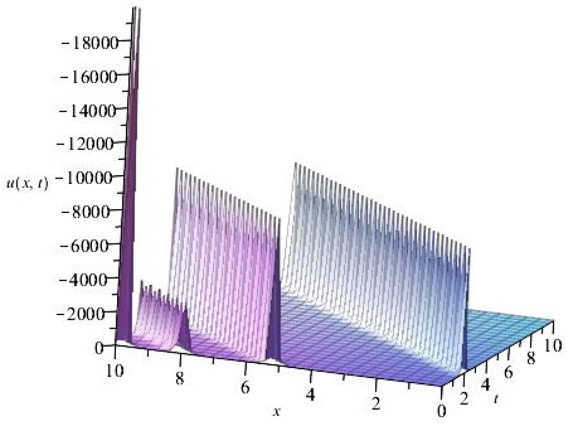
Figure 1.
Solution (9), for .
Figure 1.
Solution (9), for .

Figure 2.
Solution (12) for and .
Figure 2.
Solution (12) for and .

Publisher’s Note: MDPI stays neutral with regard to jurisdictional claims in published maps and institutional affiliations. |
© 2021 by the authors. Licensee MDPI, Basel, Switzerland. This article is an open access article distributed under the terms and conditions of the Creative Commons Attribution (CC BY) license (https://creativecommons.org/licenses/by/4.0/).
Share and Cite
MDPI and ACS Style
Márquez, A.P.; Bruzón, M.S. Lie Point Symmetries, Traveling Wave Solutions and Conservation Laws of a Non-linear Viscoelastic Wave Equation. Mathematics 2021, 9, 2131. https://0-doi-org.brum.beds.ac.uk/10.3390/math9172131
AMA Style
Márquez AP, Bruzón MS. Lie Point Symmetries, Traveling Wave Solutions and Conservation Laws of a Non-linear Viscoelastic Wave Equation. Mathematics. 2021; 9(17):2131. https://0-doi-org.brum.beds.ac.uk/10.3390/math9172131
Chicago/Turabian StyleMárquez, Almudena P., and María S. Bruzón. 2021. "Lie Point Symmetries, Traveling Wave Solutions and Conservation Laws of a Non-linear Viscoelastic Wave Equation" Mathematics 9, no. 17: 2131. https://0-doi-org.brum.beds.ac.uk/10.3390/math9172131
Note that from the first issue of 2016, this journal uses article numbers instead of page numbers. See further details here.