
A Novel MADM Framework under q-Rung Orthopair Fuzzy Bipolar Soft Sets


1
Department of Mathematics, Division of Science and Technology, University of Education, Lahore 54770, Pakistan
2
Department of Mathematics, King Saud University, Riyadh 11451, Saudi Arabia
3
Department of Logistics, Military Academy, University of Defence in Belgrade, 11000 Belgrade, Serbia
4
School of Mathematics, Xiamen University, Xiamen 361005, China
*
Author to whom correspondence should be addressed.
Mathematics 2021, 9(17), 2163; https://0-doi-org.brum.beds.ac.uk/10.3390/math9172163
Submission received: 29 June 2021
/
Revised: 14 August 2021
/
Accepted: 24 August 2021
/
Published: 4 September 2021
(This article belongs to the Special Issue Multiple Criteria Decision Making)
Abstract
:In many real-life problems, decision-making is reckoned as a powerful tool to manipulate the data involving imprecise and vague information. To fix the mathematical problems containing more generalized datasets, an emerging model called q-rung orthopair fuzzy soft sets offers a comprehensive framework for a number of multi-attribute decision-making (MADM) situations but this model is not capable to deal effectively with situations having bipolar soft data. In this research study, a novel hybrid model under the name of q-rung orthopair fuzzy bipolar soft set (q-ROFBSS, henceforth), an efficient bipolar soft generalization of q-rung orthopair fuzzy set model, is introduced and illustrated by an example. The proposed model is successfully tested for several significant operations like subset, complement, extended union and intersection, restricted union and intersection, the ‘AND’ operation and the ‘OR’ operation. The De Morgan’s laws are also verified for q-ROFBSSs regarding above-mentioned operations. Ultimately, two applications are investigated by using the proposed framework. In first real-life application, the selection of land for cropping the carrots and the lettuces is studied, while in second practical application, the selection of an eligible student for a scholarship is discussed. At last, a comparison of the initiated model with certain existing models, including Pythagorean and Fermatean fuzzy bipolar soft set models is provided.
1. Introduction
Nowadays, MADM is playing a vital role in dealing with the vague information having multi-attributes by offering better mathematical modeling in case of various real-life problems. Actually, such kinds of issues arise in Social Sciences, Medical Sciences, Environmental Sciences, Engineering, Ecology, Economics, and several different domains, which are highly dependent on the target of modeling uncertainties that cannot be solved using traditional mathematical theories, including probability theory. A good decision exhibits proper illustration of a dataset and helps to move further in the right direction. Zadeh [1] was credited for proposing the fuzzy set theory to deal with uncertain information and for introducing new research directions in several domains of science and technology, especially, decision-making. He assigned the objects by the belongingness (membership) grades in the real-valued interval . However, it was observed that some other extensions was also required to deal with non-belongingness (dissatisfaction) values of objects in different vague and uncertain situations. Later, Atanassov [2] generalized fuzzy sets and put forward the idea of intuitionistic fuzzy set (IFS) via belongingness and non-belongingness grades whose sum lies in . The theory of IFSs has rich potential applications in various domains ranging from medical to engineering. However, in some practical decision-making situations, IFSs cannot be employed. For example, consider that a team of senior professors is invited to provide their opinions on the performance of employees for promotion purpose. There may be a possibility that half of them express their belongingness degrees as 0.8 with respect to a particular parameter, while the remaining provide their non-belongingness degrees as 0.6 with respect to the same parameter. This situation cannot be illustrated by the IFSs because .
After two decades of this powerful invention of IFSs, Yager [3] was the first who presented a natural extension of IFSs called Pythagorean fuzzy sets (PFSs) in 2013, because IFSs were not sufficient for handling the data involving belongingness and non-belongingness grades whose sum does not lie in . PFSs came with a major feature that the sum of squares of belongingness and non-belongingness grades bounded by 1, which actually provided more space to this model for dealing with numerous real-life problems, i.e., in the above-mentioned situation, PFSs work well because . Note that PFSs are equivalent to the Atanassov’s IFSs of second type [4]. With the production of PFSs, many researchers put forward their attention to this fruitful model and introduced several useful results by generalizing this concept or by its implementation to different uncertainty theories. For example, Yager and Abbasov [5] discussed about an association between Pythagorean membership values and complex numbers. In order to solve MADM situations with PFSs, Zhang and Xu [6] presented an extended TOPSIS approach based on PFSs. Yager [7] presented a number of aggregation operators based on PFSs to solve the decision-making problems. Peng and Yang [8] studied subtraction and division of PFSs and discussed their significant properties. The same authors [9] introduced interval-valued PFSs as a natural generalization of PFSs.
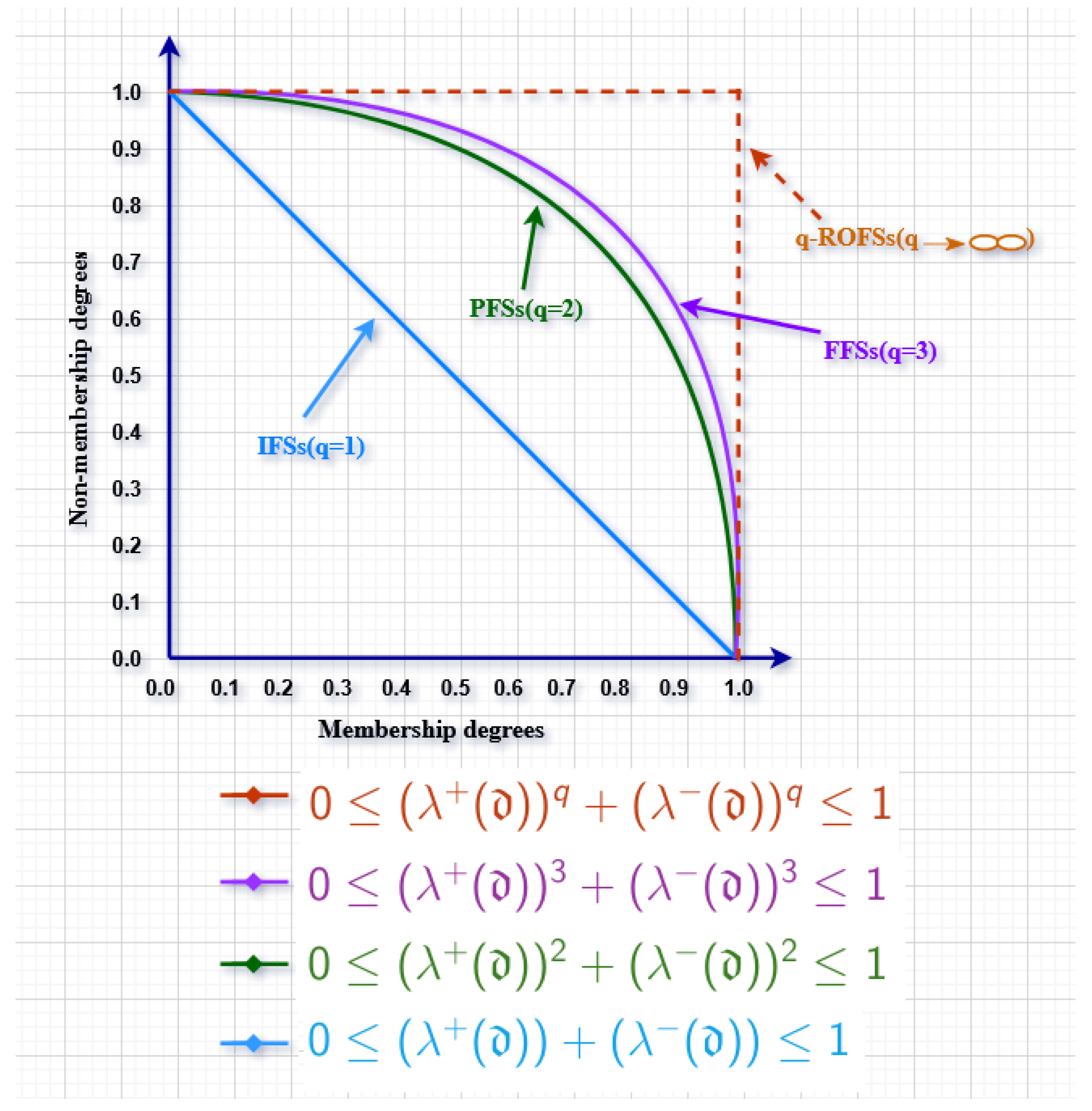
In the last few decades, many scholars attracted towards MADM methods to determine some more generalized novel mathematical tools for dealing with different types of uncertainties in numerous real-world problems. MADM models explain how attributes information is to be processed to compute a suitable object or ranking order of the objects to support decision-making. In the literature, MADM methods have been used in different domains, including engineering. No doubt, PFS theory is playing a significant role in solving of different real-world MADM problems but there is still a flaw in this model, that is, PFS fails to deal a situation where the sum of the square of belongingness and non-belongingness values is not bounded by one. To overcome this issue, Yager’s [10] contribution came in the form of q-rung orthopair fuzzy sets (q-ROFSs) with the characteristic of the sum of the qth power of belongingness and non-belongingness values of elements not being more than one. The q-ROFSs are generally reduced to IFSs [2], PFSs [3], and Fermatean fuzzy sets (FFSs) [11] for and , respectively (see Figure 1). A number of problems have been solved by using q-ROFS model. For instance, Hussain et al. [12] proposed the q-rung orthopair fuzzy soft aggregation operators and discussed their multi-criteria decision-making applications. The q-ROFS model was found to be more effective when extended to range of parameterizations and used in different domains [13,14,15,16].
Pawlak [17] initiated the theory of rough sets to handle imprecise data while he was working on the problems related to intelligent systems. According to him, different parameterized values help experts in establishing an opinion during a variety of decision-making problems. The theories of both fuzzy and rough sets suffer from the drawback of not being able to describe the consideration of multiple parameters. To resolve this issue, Molodtsov [18], in 1999, proposed a new set, known as soft set (SS). This set was mainly centered on application of mathematical models for handling vague information by means of parametric perspective. Ali et al. [19], then extended the known literature and introduced a number of new notions. They further claimed that De Morgan’s laws were applicable for SSs. They also paved way for a new direction in this field by linking several ideas to the notion of SSs. After that, Maji et al. [20,21] used SSs to define fuzzy soft sets (FSSs) and intuitionistic fuzzy soft sets (IFSSs). Since then, a host of research was published based on different aspects of FSSs and IFSSs and these sets were effectively used in decision-making for real-life problems [22,23,24]. Recently, Hamid et al. [13] proposed a new model called q-rung orthopair fuzzy soft sets (q-ROFSSs) by combining q-ROFSs with SSs.
Due to the existence of bipolar information in several practical situations, Shabir and Naz [25] extended their applications to bipolar soft sets (BSSs) and elaborated their algebraic structures. This concept was built to distinguish between preferred and adverse sides of the data. Dubois and Prade [26] introduced the role of polarity to give the reason for the positive and negative sides of alternatives. Currently, the hybrid environment of BSSs in decision-making problems has been used frequently [27,28,29]. Very recently, Ali and Ansari [30] presented a novel MADM model, namely, Fermatean fuzzy BSSs together with its two applications, including selection of a best surgeon robot and evaluation of the most affected country due to coronavirus disease 2019 (COVID-19). The existing models, namely, IFS, PFS, FFS, q-ROFS, IFSS, and q-ROFSS often lack in precision regarding bipolar soft knowledge when they come to decision-making with imprecise data. It can be elucidated from the above discussion that a hybrid model having the ability to depict bipolarity of soft data with q-rung orthopair fuzzy information is still unattended. Keeping in view the shortcomings of the existing systems, we offer a new direction for the research in the emerging era of decision-making techniques. For other useful terminologies the readers are suggested to [31,32,33,34,35,36].
The motivations of the proposed model are elaborated as follows:
- The main feature of FFSs to handle the uncertainties in people decisions make it more cogent and efficient because FFSs deal with two dimensional (i.e., belongingness and non-belongingness) information in more wider space than IFSs and PFSs;
- BSSs and q-ROFSs are two different mathematical models to address uncertain MADM situations. Therefore, there is a need of such hybrid model which have characteristics of both these models;
- The existing PFBSS model is inefficient to solve decision-making problems in which an expert evaluates the given information with the satisfactory and unsatisfactory degrees, whose sum of squares is not less than 1. To provide more space for evaluation values, the q-ROFBSS model is established, in which the sum of qth power of satisfactory and unsatisfactory degrees should be bounded by 1. Thus, q-ROFBSSs are more flexible for different vague environments as compared to certain existing models.
The major contributions of this research article are provided as below:
- Our work focuses on the improvement of efficiency of q-ROFBSS model by increasing the number of acceptable orthopairs. The illustration of the proposed work comes with an example;
- To investigate our hybrid model, we propose subset, complement, extended union and intersection, restricted union and intersection, and OR and AND operations;
- Certain De Morgan’s laws for q-ROFBSSs are also verified;
- Ultimately, we combine these ideas and offer an application with algorithm regarding selection of land for cropping carrots and lettuces. We also use this model to offer another application to help in the selection of an eligible student for scholarship;
- Furthermore, a comparison analysis with some existing models in qualitative and quantitative formats is provided;
- At the end, some concluding remarks and future directions are given.
This paper is organized as: In Section 2, some fundamental notions are reviewed, including BSSs, q-ROFSs, and q-ROFSSs. In Section 3, q-ROFBSSs are discussed along with several significant operations for q-ROFBSSs, namely, subsets, complement, extended union and intersection, restricted union and intersection, and OR and AND operations. In Section 4, two applications are investigated by using the proposed framework. Section 5 gives comparison of the developed model with certain existing models, including Pythagorean and Fermatean fuzzy BSSs. In Section 6, some concluding remarks and future directions are given.
2. Preliminaries
This section recalls some fundamental notions, namely, BSS, q-ROFSS, and q-ROFS with score and accuracy functions.
Definition 1
([25]). Let be a universal set and P be a universe of parameters. For every , a triple is called a bipolar soft set or BSS on , where f and g are functions defined as
such that , where is the ‘Not set’ of parameters.
Definition 2
([10]). Let be a universal set. Then, a pair is called the q-rung orthopair fuzzy set or q-ROFS over , where is a belongingness function given by and is a non-belongingness function given by with where . In set form, a q-ROFS on is defined as
where denotes the belongingness and non-belongingness values, respectively, and satisfies . Moreover, is known as a q-rung orthopair fuzzy number (q-ROFN) and denoted by . The degree of hesitance for q-ROFN is defined as
Assume that is the family of all q-ROFSs on .
Definition 3
Definition 4
Definition 5.
([15]). Let and be any two q-ROFNs, and be the score functions of and , and and be the accuracy functions of and , then
- if then ,
- if and
- if then ,
- if then .
Definition 6
([13]). Let and P be the universal set and universe of parameters, respectively. Assume that , then the pair is said to be a q-rung orthopair fuzzy soft set or q-ROFSS over , if A is a mapping given as . Consider and , then is a q-ROFS on , which is defined as
where denotes the belongingness and non-belongingness values, respectively, and satisfy .
3. -Rung Orthopair Fuzzy Bipolar Soft Sets
This section provides a novel hybrid structure by the mixture of BSSs and q-ROFSs which is named as q-ROFBSSs. Here, we also present some operations and then investigate by means of numerical examples.
Definition 7.
Consider a universal set and P a universe of parameters. For any , a triplet is called a q-rung orthopair fuzzy bipolar soft set or q-ROFBSS over , if and are mappings given as and , respectively, and satisfy
for all , and . Moreover, and are belongingness and non-belongingness values of an object ‘’ over and for any satisfy
respectively.
On the other hand, a q-ROFBSS over gives two parameterized q-rung orthopair fuzzy subsets on , which satisfy the Equations (3) and (4). For any , and are described as the sets of r- and -approximate elements of the q-ROFBSS , respectively.
The following example illustrate the Definition 7 precisely.
Example 1.
Let be the set of four refrigerators from different companies. Ahmad wants to buy a refrigerator. Consider the attribute set for the objects is given by
Denote the “Not set of P” as
For , we define a q-ROFBSS with q = 5, which describe the requirements of Ahmad about the refrigerator, he wishes to buy. Then, a 5-ROFBSS is given by
The 5-ROFBSS can be represented in tabular form as shown in Table 1.
Thus, is a 5-ROFBSS based on expensiveness, attractiveness, and few other parameters associated with the selection of refrigerator. For instance, from Table 1, represents that the support of the belongingness of refrigerator is and is the support against belongingness of based expensiveness. In a similar manner, for the parameter ‘cheap’ which gives totally opposite meaning to the parameter ‘expensive’, is the belongingness degree in the support of , and is the belongingness degree against the support of based cheapness.
Remark 1.
Basic Operations
In this subsection, we explore some basic notions of q-ROFBSSs and investigate them with corresponding numerical examples.
Definition 8.
Let be a universal set and , be two q-ROFBSSs over . The set is called a q-rung orthopair fuzzy bipolar soft subset of , denoted as , if
- ,
- (that is, and (that is, for all and .
Example 2.
Let 5-ROFBSS on be as defined in Example 1, for , , we give a new 5-ROFBSS , which is given by Table 4:
It is clear from Definition 8 that .
Definition 9.
Let be a universal set. Consider and are two q-ROFBSSs over . Then, and are said to be equal, if and .
Definition 10.
Let be a universal set and be a q-ROFBSS. Then, its complement is a q-ROFBSS over with and for all and .
Example 3.
Let be the 5-ROFBSS over a universe as considered in Example 1. Then, by Definition 10, its complement is computed in Table 5.
Definition 11.
A q-ROFBSS on a universe is refereed to as a relative null q-ROFBSS, represented by if and ∀ .
Definition 12.
A q-ROFBSS on a universe is refereed to as a relative absolute q-ROFBSS, represented by if and ∀ .
Definition 13.
Let and be two q-ROFBSSs over a universe . Then, the “AND” operation on and , denoted by , is defined as where for all , , and ,
Definition 14.
Let and be two q-ROFBSSs over a universe . Then the “OR” operation on and , denoted by , is defined as where for all , , and ,
Example 4.
The following proposition describes that certain De Morgan’s laws verify with the AND operation and the OR operation.
Proposition 1.
Let be a universe and let and be q-ROFBSSs on . Then
Proof.
- 1.
- From Definitions 10 and 14, where and for all and .Now by using Definition 10, and . Therefore, (by Definition 13) where and for all and . Thus,
- 2.
- It proof is similar to part 1.
□
Definition 15.
Let and be two q-ROFBSSs on . Then, the extended union of and , represented by , is a q-ROFBSS , , on , defined as follows:
where
Definition 16.
Let and be two q-ROFBSSs over . Then, the restricted union of and , denoted by , is a q-ROFBSS , , on , where for all and for all , provided , .
Definition 17.
Let and be two q-ROFBSSs over . Then, the extended intersection of and , represented by , is a q-ROFBSS , , on , defined as follows:
where
Definition 18.
Let and be any two q-ROFBSSs over a universe . Then, the restricted intersection of and , represented by , is a q-ROFBSS on , where for all and for all , provided , .
Example 5.
Let be a 7-ROFBSS over , with given by Table 10 and be the 7-ROFBSS on the universe , as considered in Example 4. Then, their extended union and the extended intersection are, respectively, displayed in Table 11 and Table 12. The tabular arrangements of the restricted intersection and union are provided by Table 13 and Table 14, respectively.
Lemma 1.
Let and be two q-ROFBSSs on a universe . Then
- is the smallest q-ROFBSS over which contains both and ;
- is the largest q-ROFBSS over which is subset of both and .
Proof.
Straightforward. □
In the following theorem, we verify that certain De Morgan’s laws hold with the extended (restricted) union and intersection.
Theorem 1.
Let and be two q-ROFBSSs on the universe . Then,
Proof.
- By Definition 10 and 15, we obtain , whereHence, .The remaining parts (2–4) can be easily followed. □
Here, we define a q-rung orthopair fuzzy weighted average operator to aggregate the q-rung orthopair fuzzy information.
Definition 19.
Let be a family of q-ROFNs and every be related with an important weight , such that , then the q-rung orthopair fuzzy weighted average (q-ROFWA) operator is given by
4. Applications
MADM technique plays a significant role to handle many complicated real-life decision-making situations. Here, we describe two practical applications with MADM method based on q-ROFBSSs.
4.1. Selection of Land for Cropping Carrots and Lettuces
With the growing world population the food demands are increasing day-by-day. Crops play a major role to fulfill these food requirements. There are various factors involve in the development of crops production, like soil condition, environment, etc. Actually, soil condition is a very important part in the production process of any crop. The fertility of land is very important for good yield of any crop. For instance, land containing clay soil is not suited for various vegetables and field crops like wheat, rice, etc. However, fruit trees, ornamental trees and shrubs can thrive on clay soil. Therefore, the land selection is very significant for the crops growth because a crop production may vary from one land piece to another. It is an uncertain problem for agriculture experts to choose best land for crops development. That is why, we investigate this daily-life problem by applying our proposed methodology.
Suppose a farmer wants to buy a land, through a land dealer company, which should be suitable for the cropping of carrots and lettuces. According to the dealer, a land with high porosity (i.e., land with many pores so that water can penetrate through soil pores easily), good soil texture, neutral pH (i.e., neither basic nor acidic), and even colour soil is suitable for farmer. There are fifteen lands which make the set of alternatives, . According to the company, consider be a set of parameters. For the parameters stand for “good soil texture”, “crumbly soil”,“high porosity”, “neutral pH soil”, and “single colour soil”, respectively. Let the ‘Not set of P’ be . After a detailed discussion among the committee members of dealer company, they decide the evaluation of every piece of land will be done with a favorable subset of P. According to the committee, the q-ROFBSS with q = 4 describes the “requirements of the lands” which is given by Table 15 below.
Based on the significant of every parameter , the committee gives a specific weight to each parameter which are:
By using q-ROFWA operator (see Definition 19), we calculate
Similarly,
Now
Similarly,
By Definition 3, we have
Now, the final scores are computed as:
Clearly, is the optimal alternative. Therefore, the committee will suggest the farmer to buy the land for cropping carrots and lettuces.
The algorithm based on q-ROFBSSs for the selection process of most appropriate option is given as below (see Algorithm 1):
| Algorithm 1: Selection of a suitable object using q-ROFBSSs |
Input:
|
Now we apply our developed model to another real situation under q-ROFBSSs.
4.2. Selection of Student for Scholarship
The basic process for evaluating applicants and awarding scholarships depends on different factors which are surely uncertain. For instance, financial information about the applicant is an important factor for awarding a scholarship. It is possible that a student who is not deserving may provide incorrect financial information. Then, it is on the experts (interviewers) to decide whether he or she is deserving or not. Thus, it is an uncertain problem. Similarly, there exist many other factors which effects the selection procedure of deserving and brilliant students for scholarships, such as morality, honesty, etc.
Suppose the Higher Education Commission (HEC) of Pakistan announces a merit and need based scholarship for undergraduate students of universities. This task is given to a team of 5 senior employees. Consider there are twenty applicants from a university XYZ which make the set of alternatives, . According to the HEC, let be a set of parameters for the selection of candidates for scholarships. For the parameters serve as “high CGPA”, “Good Character”, “Poor financial state”, “punctual”and “cooperative”, respectively. Let the ‘Not set of P’ be . With a brief discussion among the members of selection team appointed by HEC, they decide that the evaluation of every applicant will be done with a favorable subset of parameters of P. According to the team members, the q-ROFBSS with q = 5 describes the “qualities of the students” which are displayed in the Table 16 below.
Based upon the significant of every parameter , the team members give a specific weight to each parameter which are:
By using q-ROFWA operator (see Definition 19), we calculate
Similarly,
Now
Similarly,
By Definition 3, we have
Additionally, we get
Now we compute the final score values as follows:
Clearly, is the most suitable student. Therefore, the HEC will select student for the merit and need based scholarship.
5. Sensitivity Analysis
To prove the efficiency and cogency of the developed q-ROFBSS model, this section discusses its advantages and comparative analysis with PFBSSs [28] and FFBSSs [30].
- Advantages: A quick analysis of recent years show that a rapid progress has been done for dealing with uncertain information in many MADM situations which is the evidence of this fruitful era. Due to the existence of various practical MADM situations in this universe, it is a wish of every researcher to establish a new model or its hybridized version. It is a limitless approach. Currently, BSS model and its fuzzy and Pythagorean fuzzy formats are arising as very powerful tools but a generalized fuzzy version of these models is not introduced yet. With the motivation of these facts, a new hybrid model, namely, q-ROFBSSs is presented which have ability to deal with many real situations involving q-rung orthopair fuzzy bipolar soft knowledge. The developed q-ROFBSS approach is more efficient and flexible to tackle vague information in different MADM problems. Particularly, if the given information involving parameters with opposite meanings. It can be easily see that existing MADM models, i.e., fuzzy BSS model is not capable to consider the non-belongingness values of alternatives in a MADM problem while PFBSS model is not able to handle the belongingness and non-belongingness degrees whose sum of their squares is not bounded by 1. Thus, developed q-ROFBSS method has ability to handle both fuzzy and Pythagorean fuzzy bipolar soft information.
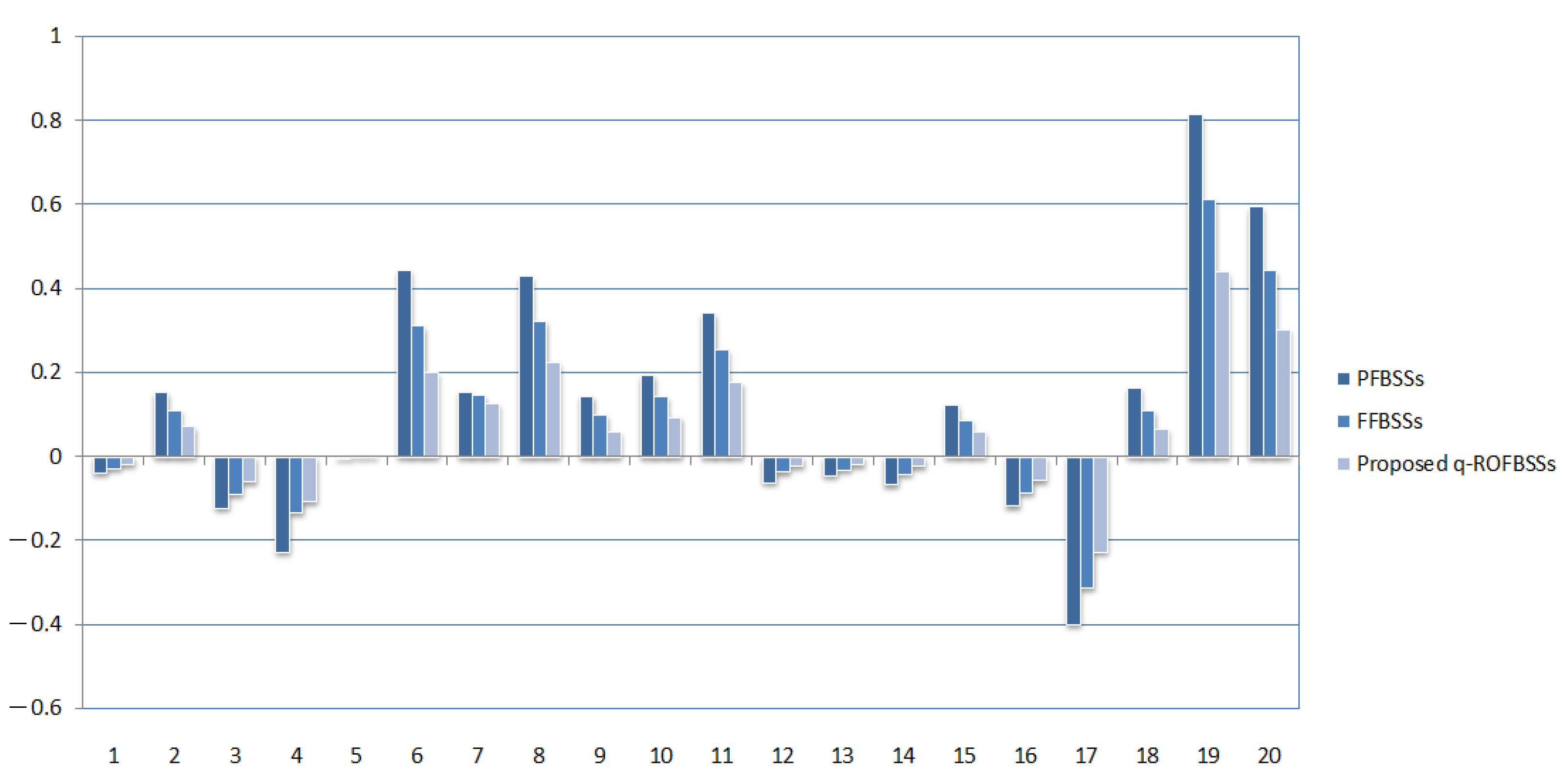
- Comparison: The production of IFSs and PFSs is enough to show the importance of non-membership function in different real situations. However, there are some limitations of these models, such as they fail to handle the MADM problems in which the sum of squares of belongingness and non-belongingness values is greater than 1. In these days, to solve such critical problems, q-ROFSs are arising as more flexible tool as compared to IFSs and PFSs. In the literature, several soft computing models, including fuzzy BSSs [37], PFBSSs [28], FFBSSs [30] and m-polar fuzzy BSSs [29] have been introduced for dealing with different kinds of uncertain real-world MADM problems. Inspired by these facts, q-ROFBSSs are proposed to deal with different fuzzy versions of bipolar soft information. Our proposed model provided more space to belongingness and non-belongingness degrees as compared to FBSSs [37] and PFBSSs [28]. Notice that the existing MADM methods, namely, PFBSSs [28] and FFBSSs [30] fail to solve the developed applications in this study. Therefore, to check the comparison of PFBSSs [28], FFBSSs [30], and our proposed q-ROFBSS model (for ), we apply them on the data-sets of Applications 1 and 2 in [28]. From the Table 17 and Table 18, it can be easily see that not only optimal decision objects by applying these models are equal, that is and in Applications 1 and 2 of [28], respectively, but also ranking order are similar (for more clarification see the Figure 2 and Figure 3). Thus, our presented MADM hybrid model is more flexible and efficient than certain existing models, including PFBSSs [28] and FFBSSs [30].
6. Conclusions
Decision-making performs a significant role in mathematical modeling to refine the selection of logical attributes in almost every real-life problem. In this study, we have proposed a novel hybrid model called q-ROFBSSs for MADM by combining q-ROFSs and BSSs. The developed model leads us to use parametrization tool regarding bipolarity during problem-solving as compared to existing mathematical tools for dealing with uncertain information. Furthermore, we have described some fundamental operations defined on q-ROFBSSs and investigated them with examples. We have also developed decision-making methods by the means of novel constructions in Section 3. Moreover, we have provided justification of our proposed work by solving two real-world problems involving uncertain information, which are: (a) selection of land for cropping the carrots and the lettuces; (b) selection of eligible student for scholarship. Hence, it is observed that hybridization of different models make us able to get more accurate and best information than other existing models. In last, we have studied a comparison analysis of developed approach with certain existing models, including Pythagorean and Fermatean fuzzy BSS models. The presented work can therefore be extended in the following lines:
- q-rung orthopair fuzzy bipolar soft sets can be generalized to interval-valued q-rung orthopair fuzzy bipolar soft sets to evaluate different MADM problems more effectively;
- A novel hybrid model, namely, q-rung orthopair picture fuzzy bipolar soft sets can be established by combining q-rung orthopair fuzzy bipolar soft sets and picture fuzzy sets;
- q-rung orthopair fuzzy bipolar soft sets can be extended to q-rung orthopair fuzzy bipolar soft expert sets to solve different group decision-making problems.
Author Contributions
Conceptualization, G.A., H.A., D.P., M.A. and N.L.; methodology, G.A., H.A., D.P., M.A. and N.L.; validation, G.A., H.A. and D.P.; formal analysis, G.A. and H.A.; investigation, G.A., D.P. and N.L.; data curation, G.A., H.A., D.P. and N.L.; writing—original draft preparation, G.A., H.A. and N.L.; writing—review and editing, G.A., H.A., D.P., M.A. and N.L.; visualization, G.A., H.A., D.P. and M.A.; supervision, G.A., H.A. and D.P.; project administration, G.A., H.A. and D.P.; funding acquisition, H.A. All authors have read and agreed to the published version of the manuscript.
Funding
This work is supported by the Researchers Supporting Project number (RSP-2021/317), King Saud University, Riyadh, Saudi Arabia.
Institutional Review Board Statement
Not applicable.
Informed Consent Statement
Not applicable.
Data Availability Statement
Not applicable.
Conflicts of Interest
The authors declare no conflict of interest.
References
- Zadeh, L.A. Fuzzy sets. Inf. Cont. 1965, 8, 338–353. [Google Scholar] [CrossRef] [Green Version]
- Atanassov, K.T. Intuitionistic fuzzy sets. Fuzzy Sets Syst. 1986, 20, 87–96. [Google Scholar] [CrossRef]
- Yager, R.R. Pythagorean fuzzy subsets. In Proceedings of the 2013 Joint IFSA World Congress and NAFIPS Annual Meeting (IFSA/NAFIPS), Edmonton, AB, Canada, 24–28 June 2013; pp. 57–61. [Google Scholar]
- Atanassov, K.T. Intuitionistic Fuzzy Sets-Theory and Applications; Springer: New York, NY, USA, 1999. [Google Scholar]
- Yager, R.R.; Abbasov, A.M. Pythagorean membership grades, complex numbers, and decision making. Int. J. Intell. Syst. 2013, 28, 436–452. [Google Scholar] [CrossRef]
- Zhang, X.; Xu, Z. Extension of TOPSIS to multiple criteria decision making with Pythagorean fuzzy sets. Int. J. Intell. Syst. 2014, 29, 1061–1078. [Google Scholar] [CrossRef]
- Yager, R.R. Pythagorean membership grades in multi-criteria decision making. IEEE Trans. Fuzzy Syst. 2014, 22, 958–965. [Google Scholar] [CrossRef]
- Peng, X.; Yang, Y. Some results for Pythagorean fuzzy sets. Int. J. Intell. Syst. 2015, 30, 1133–1160. [Google Scholar] [CrossRef]
- Peng, X.; Yang, Y. Fundamental properties of interval-valued Pythagorean fuzzy aggregation operators. Int. J. Intell. Syst. 2016, 31, 444–487. [Google Scholar] [CrossRef]
- Yager, R.R. Generalized orthopair fuzzy sets. IEEE Trans. Fuzzy Syst. 2016, 25, 1222–1230. [Google Scholar] [CrossRef]
- Senapati, T.; Yager, R.R. Fermatean fuzzy sets. J. Amb. Intell. Hum. Comput. 2020, 11, 663–674. [Google Scholar] [CrossRef]
- Hussain, A.; Ali, M.I.; Mahmood, T.; Munir, M. q-Rung orthopair fuzzy soft average aggregation operators and their application in multicriteria decision-making. Int. J. Intell. Syst. 2020, 35, 571–599. [Google Scholar] [CrossRef]
- Hamid, M.T.; Riaz, M.; Afzal, D. Novel MCGDM with q-rung orthopair fuzzy soft sets and TOPSIS approach under q-Rung orthopair fuzzy soft topology. J. Intell. Fuzzy Syst. 2020, 39, 3853–3871. [Google Scholar] [CrossRef]
- Li, L.; Lei, H.; Wang, J. q-Rung probabilistic dual hesitant fuzzy sets and their application in multi-attribute decision-making. Mathematics 2020, 8, 1574. [Google Scholar] [CrossRef]
- Liu, P.; Wang, P. Some q-rung orthopair fuzzy aggregation operators and their applications to multiple-attribute decision making. Int. J. Intell. Syst. 2018, 33, 259–280. [Google Scholar] [CrossRef]
- Peng, X.; Huang, H.; Luo, Z. q-Rung orthopair fuzzy decision-making framework for integrating mobile edge caching scheme preferences. Int. J. Intell. Syst. 2021, 36, 2229–2266. [Google Scholar] [CrossRef]
- Pawlak, Z. Rough sets. Int. J. Comput. Inf. Sci. 1982, 11, 341–356. [Google Scholar] [CrossRef]
- Molodtsov, D.A. Soft set theory-First results. Comput. Math. Appl. 1999, 37, 19–31. [Google Scholar] [CrossRef] [Green Version]
- Ali, M.I.; Feng, F.; Liu, X.Y.; Min, W.K.; Shabir, M. On some new operations in soft set theory. Comput. Math. Appl. 2009, 57, 1547–1553. [Google Scholar] [CrossRef] [Green Version]
- Maji, P.K.; Biswas, R.; Roy, A.R. Fuzzy soft sets. J. Fuzzy Math. 2001, 9, 589–602. [Google Scholar]
- Maji, P.K.; Biswas, R.; Roy, A.R. Intuitionistic fuzzy soft sets. J. Fuzzy Math. 2001, 9, 677–692. [Google Scholar]
- Alcantud, J.C.R.; Khameneh, A.Z.; Kilicman, A. Aggregation of infinite chains of intuitionistic fuzzy sets and their application to choices with temporal intuitionistic fuzzy information. Inf. Sci. 2020, 514, 106–117. [Google Scholar] [CrossRef]
- Feng, F.; Jun, Y.B.; Liu, X.; Li, L. An adjustable approach to fuzzy soft set based decision-making. J. Comput. Appl. Math. 2010, 234, 10–20. [Google Scholar] [CrossRef] [Green Version]
- Feng, F.; Fujita, H.; Ali, M.I.; Yager, R.R.; Liu, X. Another view on generalized intuitionistic fuzzy soft sets and related multi attribute decision making methods. IEEE Trans. Fuzzy Syst. 2018, 27, 474–488. [Google Scholar] [CrossRef]
- Shabir, M.; Naz, M. On bipolar soft sets. arXiv 2013, arXiv:1303.1344. [Google Scholar]
- Dubois, D.; Prade, H. An introduction to bipolar representations of information and preference. Int. J. Intell. Syst. 2008, 23, 866–877. [Google Scholar] [CrossRef]
- Malik, N.; Shabir, M. Rough fuzzy bipolar soft sets and application in decision-making problems. Soft Comput. 2019, 23, 1603–1614. [Google Scholar] [CrossRef]
- Akram, M.; Ali, G. Hybrid models for decision-making based on rough Pythagorean fuzzy bipolar soft information. Granul. Comput. 2020, 5, 1–15. [Google Scholar] [CrossRef]
- Akram, M.; Ali, G.; Shabir, M. A hybrid decision-making framework using rough mF bipolar soft environment. Granul. Comput. 2021, 6, 539–555. [Google Scholar] [CrossRef]
- Ali, G.; Ansari, M.N. Multiattribute decision-making under Fermatean fuzzy bipolar soft framework. Granul. Comput. 2021. [Google Scholar] [CrossRef]
- Akram, M.; Ali, G.; Alcantud, J.C.R. Parameter reduction analysis under interval-valued m-polar fuzzy soft information. Art. Intell. Rev. 2021. [Google Scholar] [CrossRef]
- Ali, G.; Akram, M. Decision-making method based on fuzzy N-soft expert sets. Arab. J. Sci. Eng. 2020, 45, 10381–10400. [Google Scholar] [CrossRef]
- Hu, X.; Yang, S.; Zhu, Y.R. Multiple Attribute Decision-Making Based on Three-Parameter Generalized Weighted Heronian Mean. Mathematics 2021, 9, 1363. [Google Scholar] [CrossRef]
- Liu, D.; Huang, A.; Liu, Y.; Liu, Z. An extension TOPSIS method based on the decision maker’s risk attitude and the adjusted probabilistic fuzzy set. Symmetry 2021, 13, 891. [Google Scholar] [CrossRef]
- Yang, M.S.; Ali, Z.; Mahmood, T. Three-way decisions based on q-rung orthopair fuzzy 2-tuple linguistic sets with generalized Maclaurin symmetric mean operators. Mathematics 2021, 9, 1387. [Google Scholar] [CrossRef]
- Wang, H.; Zhang, Y.; Yao, J. An extended VIKOR method based on q-rung orthopair shadowed set and its application to multi-attribute decision making. Symmetry 2020, 12, 1508. [Google Scholar] [CrossRef]
- Naz, M.; Shabir, M. On fuzzy bipolar soft sets, their algebraic structures and applications. J. Intell. Fuzzy Syst. 2014, 26, 1645–1656. [Google Scholar] [CrossRef]

Figure 2.
Comparison between PFBSSs [28], FFBSSs [30], and proposed q-ROFBSSs by applying on Application 1 (Selection of an employee) in [28].

Figure 3.
Comparison between PFBSSs [28], FFBSSs [30], and proposed q-ROFBSSs by applying on Application 2 (Selection of a house) in [28].


Table 1.
Table for the 5-ROFBSS .
Table 2.
Table for belongingness and non-belongingness values for the parameter set .
| (0.8, 0.9) | (0.6, 0.9) | (0.6, 0.7) | |
| (0.7, 0.6) | (0.5, 0.5) | (0.4, 0.5) | |
| (0.4, 0.9) | (0.6, 0.3) | (0.9, 0) | |
| (0.98, 0.3) | (0.9, 0.1) | (0.7, 0.8) |
Table 3.
Table for belongingness and non-belongingness values for the set .
| (0.2, 0.1) | (0.4, 0.1) | (0.4, 0.3) | |
| (0.3, 0.3) | (0.5, 0.4) | (0.6, 0.5) | |
| (0.5, 0.1) | (0.4, 0.7) | (0.1, 0.9) | |
| (0.01, 0.7) | (0.1, 0.8) | (0.3, 0.2) |
Table 4.
Table for the 5-ROFBSS .
Table 5.
Table for the complement of .
Table 6.
Table for the 7-ROFBSS .
Table 7.
Table for the 7-ROFBSS .
Table 8.
Table for the 7-ROFBSS .
Table 9.
Table for the 7-ROFBSS .
Table 10.
Table for the 7-ROFBSS .
Table 11.
Table for the extended union .
Table 12.
Table for the extended intersection .
Table 13.
Table for the restricted intersection .
Table 14.
Table for the restricted union .
Table 15.
Table for the 4-ROFBSS .
Table 16.
Table for the 5-ROFBSS .
Table 17.
Comparison table for the Application 1 (Selection of an employee) in [28].
Table 17.
Comparison table for the Application 1 (Selection of an employee) in [28].
| Models | ||||||||||
| PFBSSs [28] () | ||||||||||
| FFBSSs [30] () | ||||||||||
| Proposed q-ROFBSSs () | 0.0721 | 0.004 | 0.201 | 0.127 | 0.225 | 0.060 | 0.095 | |||
| Models | ||||||||||
| PFBSSs [28] () | ||||||||||
| FFBSSs [30] () | 0.256 | |||||||||
| Proposed q-ROFBSSs () | 0.178 | 0.060 | 0.067 | 0.440 | 0.304 |
Table 18.
Comparison table for the Application 2 (Selection of a house) in [28].
Publisher’s Note: MDPI stays neutral with regard to jurisdictional claims in published maps and institutional affiliations. |
© 2021 by the authors. Licensee MDPI, Basel, Switzerland. This article is an open access article distributed under the terms and conditions of the Creative Commons Attribution (CC BY) license (https://creativecommons.org/licenses/by/4.0/).
Share and Cite
MDPI and ACS Style
Ali, G.; Alolaiyan, H.; Pamučar, D.; Asif, M.; Lateef, N. A Novel MADM Framework under q-Rung Orthopair Fuzzy Bipolar Soft Sets. Mathematics 2021, 9, 2163. https://0-doi-org.brum.beds.ac.uk/10.3390/math9172163
AMA Style
Ali G, Alolaiyan H, Pamučar D, Asif M, Lateef N. A Novel MADM Framework under q-Rung Orthopair Fuzzy Bipolar Soft Sets. Mathematics. 2021; 9(17):2163. https://0-doi-org.brum.beds.ac.uk/10.3390/math9172163
Chicago/Turabian StyleAli, Ghous, Hanan Alolaiyan, Dragan Pamučar, Muhammad Asif, and Nimra Lateef. 2021. "A Novel MADM Framework under q-Rung Orthopair Fuzzy Bipolar Soft Sets" Mathematics 9, no. 17: 2163. https://0-doi-org.brum.beds.ac.uk/10.3390/math9172163
Note that from the first issue of 2016, this journal uses article numbers instead of page numbers. See further details here.