Incorporating Fuzzy Logic in Harrod’s Economic Growth Model

Abstract

This paper suggests the possibility of incorporating the methodology of fuzzy logic theory into Harrod’s economic growth model, a classic model of economic dynamics for studying the growth of a developing economy based on the assumption that an economy with only savings and investment income is in equilibrium when savings are equal to investment. This model was the first precursor to exogenous growth models, which in turn gave rise to endogenous growth models. This article therefore represents a first step towards introducing fuzzy logic into economic growth models. The study concerned considers consumption and savings to depend on income by means of uncertain factors, and investment to depend on the variation of income through the accelerator factor, which we consider uncertain. These conditions are used to determine the equilibrium growth rate of income and investment, as well as the uncertain values for these variables in terms of fuzzy numbers. As a result, the new model is shown to expand the classical model by incorporating uncertainty into its variables.

1. Introduction

As is well known, macroeconomics studies how economic systems work from an aggregate point of view as a result of the interactions that take place between different economic agents. Given this consideration, we can state that this field of economic science has the following two aims:

(a)

To investigate and clarify situations that have taken place and study what may have caused them. These prior experiences should allow us to devise mathematical models that can help explain economic reality;

(b)

To put forth predictions, usually in the short and medium run, related to how certain economic variables evolve, including national income, investment, consumption, among others. Consequently, mathematical models created from past experiences must be empirically tested in order to show their suitability for representing the reality studied and thus evaluating that the predictions with the models are reliable.

All economic models rely on a theoretical basis that tries to simplify the complexity of economic systems by stating a set of relationships between variables linked by parameters that are a priori unknown (but in certain cases can be estimated econometrically). The dependence of the model on several parameters implies that when it is necessary to determine the adequacy of the model to reality, the exact values of most of the parameters embedded in the model are not known. This involves taking uncertain quantities in the models as defined, and thus, when the model is applied, a result close to the empirical reality is already expected, but in practice it can often be wrong. Solow [1] already warns of this fact with the statements “all theory depends on assumptions which are not quite true”, and “the art of successful theorizing is to make the inevitable simplifying assumptions in such a way that the final results are not very sensitive”. The aim of this article is to present a complementary and novel point of view, introducing a fuzzy logic model in order to obtain results based on an infinity of possible inputs. This new modelling based on fuzzy logic [2] allows that empirical reality can be one of the expected results of the model and therefore the actual result is not expected to be outside the range of possible expected values. To sum up, the idea is not to check how much we have deviated from the actual solution with the model, but to confirm that this actual solution is one of the possible solutions derived in the model.

In order to limit the set of possible solutions yielding the best forecast, it is common to resort to certain constructs of the theory of fuzzy sets, known as fuzzy numbers, and which can be associated with numerical values with a degree of possibility [3]. The idea of considering the future in a pessimistic, optimistic and highly plausible scenario is the basis of these types of numbers that collect all values with some degree of possibility greater than zero. It is the ease of use of these mathematical structures [4,5,6,7] that allows uncertainty to be incorporated efficiently into any economic model regarding the behavior of economic, social and financial scenarios. This is especially necessary when sudden changes in the values of the variables are expected due to events not reflected in the historical series.

The incorporation of fuzzy logic into economic models has been addressed in a multitude of papers [8,9,10]. Following this line of research, in recent years the fuzzy logic perspective has been proposed for various growth models [11,12]. The present work, included in this current line of research, proposes the creation of a dynamic model of income behavior based on the classic Harrod model. This model is seminal in the economic growth literature. It is well known that this model has several shortcomings [13,14]. For example, the model assumes that productive capacity is proportional to capital stock, an assumption that has been shown to be false. In fact, the model was overtaken first by the so-called “exogenous growth” models of Solow [1] and Swan [15] and then by the “endogenous growth” models [16]. Essentially, exogenous growth models explain long-term growth using a variable which exogenous to the model: technology. Endogenous growth models try to explain the way in which the evolution of technology allows long-term growth. This article recovers Harrod’s original approach in order to show how the contribution of fuzzy logic to a very simple model can change the predictions that stem from the model and bring them closer to reality. This paper must be understood, then, as a first step in a process that will have to continue with the application of fuzzy logic to exogenous growth models, first, and endogenous, later.

In order to meet our primary objective, the main body of the work has been divided into three different blocks. Section 2 presents a brief summary of the fuzzy logic tools used by the new model, specifically the method used to solve equations with fuzzy parameters. Section 3 details the initial Harrod model for determining income through the use of fuzzy parameters. The results are simplified in Section 4 to make them more operational when we analyze the particular case in which uncertain parameters are expressed through triangular fuzzy numbers (TFN). Section 5 provides a numerical example with the proposed new model. Finally, the paper ends with the conclusions and references.

2. Preliminaries

In classical set theory, a set is defined as any well-defined collection of objects. This theory highlights the fact that there can never be any doubt at all as to whether any object belongs to the set or not. If the object belongs to it, it is said to belong to the set in degree 1. If the object does not belong to it, it is said to belong to the set in degree 0, there is no other option. With the birth of fuzzy set theory [2], the membership constraint is relaxed, accepting that objects can partially belong to the set. Thus, for example, a bitten apple may belong to the set of apples in grade 0.5 [17,18]. The sets created with this approach are called fuzzy sets and make up the basic elements of Zadeh’s theory. In order to establish the nomenclature that will be used in the present paper, we proceed to define the different concepts related to fuzzy sets.

Definition 1.

Fuzzy subset, membership function and support.

We consider$E$an ordinary set that we take as referential set. A fuzzy subset$\tilde{A}$of$E$is a set of ordered pairs:

$$\tilde{A}=\left\{\left(x , {\mu }_{\tilde{A}}\left(x\right)\right)/x\in E\right\}$$

where${\mu }_{\tilde{A}}$is a function:${\mu }_{\tilde{A}} : E \to \left[0 , 1\right]$.

Function${\mu }_{\tilde{A}}$is called membership function of fuzzy subset$\tilde{A}$, and given an element$x$ ∈ $E$, the value ${\mu }_{\tilde{A}}\left(x\right)$ is called membership degree, compatibility degree or truth degree of element $x$ in fuzzy subset $\tilde{A}$.

We call Support of$\tilde{A}$, and we indicate by$Supp\left(\tilde{A}\right)$at the ordinary set:

$$Supp\left(\tilde{A}\right)=\left\{x\in E/{\mu }_{\tilde{A}}\left(x\right)>0\right\}$$

Definition 2.

Fuzzy number

A fuzzy number$\tilde{A}$is defined as a fuzzy subset of the referential R of the set of real numbers such that the membership function fulfils the following conditions:

• 1a. A minimum of value$x$exists so that${\mu }_{\tilde{A}}\left(x\right)=1$(normality)
• 1b.${\mu }_{\tilde{A}}\left(x\right)\ge min\left({\mu }_{\tilde{A}}(x_1\right), {\mu }_{\tilde{A}}\left(x_2\right))$∀$x_1$,$x_2$∈ R and ∀$x$∈ [$x_1$,$x_2$] (convexity)
• 1c.${\mu }_{\tilde{A}}\left(x\right)$is a piecewise continuous function in all the points of$ℝ$, this is, it’s a continuous function except perhaps at a finite number of points in its domain.

The fuzzy number is in accordance with a prediction made by a human being. For example, convexity guarantees that as we approach a value x the closer x₀ with ${\mu }_{\tilde{A}}\left(x_0\right)=1$, then its possibility value of this x is higher. It is important that readers are aware of this restrictive assumption.

Further, note that any real number $“m”$ (which may be referred to as a crisp number) can be considered a particular case of fuzzy number whose membership function is $\mu \left(x\right)=\{\begin{array}{c}1 if x=m\\ 0 if x\ne m \end{array}$.

It is important to know that, by virtue of the representation theorem established by Zadeh [19], every fuzzy number $\tilde{A}$ can be expressed via its α-cuts, and for this reason we can express in a simplified way:

$$\tilde{A}=\left\{A_{\alpha } , 0\le \alpha \le 1\right\}$$

(1)

where $A_{\alpha }=\left\{x\in R/{\mu }_{\tilde{A}}\left(x\right)\ge \alpha \right\}\subseteq R$.

By virtue of convexity, $A_{\alpha }$ is reduced to a closed interval of R, which shall be represented thus:

$$A_{\alpha }=\left[\underset{\_}{A}\left(\alpha \right), \overline{A}\left(\alpha \right)\right]$$

(2)

where $\underset{\_}{A}\left(\alpha \right)=min\left\{x/{\mu }_{\tilde{A}}\left(x\right)\ge \alpha \right\}$ and $\overline{A}\left(\alpha \right)=max\left\{x/{\mu }_{\tilde{A}}\left(x\right)\ge \alpha \right\}$.

Note that the representation theorem is justified in its formal form trough the following equality:

$$\tilde{A}=\underset{\alpha \in \left[0,1\right]}{{\displaystyle \cup }}\alpha ·A_{\alpha }$$

understanding the union through the maximum operator, because the membership function verifies:

$${\mu }_{\tilde{A}}\left(x\right)=\underset{\alpha \in \left[0,1\right]}{\max }\left\{\alpha ·{\mu }_{A_{\alpha }}\left(x\right)\right\}$$

We must also take into account that $\underset{\_}{A}\left(\alpha \right)$ is an increasing function with regard to α, and that $\overline{A}\left(\alpha \right)$ is a decreasing function with regard to α due to convexity.

However, just as algebraic operations can be conducted using real numbers, here our interest lies in determining how common operations on real numbers can incorporate the use of fuzzy numbers.

This can be resolved if we apply the extension principle of operations or composition laws, initially introduced by Zadeh [19], and subsequently modified by other authors [20,21,22,23], which considers a general method for extending the usual operations of arithmetic to the case in which uncertain amounts are represented through fuzzy subsets or fuzzy numbers.

In the case that we have a unary operation $f\left(a\right)$ or a binary operation $f\left(a,b\right)$ between one or two quantities respectively, which are the cases we will study in our model, we will have that the principle of extension of operations to uncertain magnitudes expressed by fuzzy subsets will represent the degree of possibility of each possible solution from the following membership functions:

• If $\tilde{A}$ is a fuzzy subset of E, the extension of a unary operation from a set $E$ to another set $F$:

  $$f:E \to F$$

will be given by the fuzzy subset $\tilde{C}=f\left(\tilde{A}\right)$ with the membership function:

$${\mu }_{\tilde{C}}\left(z\right)=\{\begin{array}{c}\underset{x\in f^{-1}\left(z\right)}{{\displaystyle \vee }}{\mu }_{\tilde{A}}\left(x\right) if f^{-1}\left(z\right)\ne \varnothing \\ 0 if f^{-1}\left(z\right)=\varnothing \end{array}$$

(3)

where ∨ represents the supremum operator.

2.

For the most common case, whereby a binary operation or internal composition law between the elements of $E$ is defined by:

$$\begin{gathered} f:E\times E \to E \\ \left(x,y\right) \to f\left(x,y\right)=x\ast y \end{gathered}$$

if we consider $\tilde{A}$ and $\tilde{B}$ as fuzzy subsets of $E$, then $\tilde{C}=f(\tilde{A} , \widetilde{B)}=\tilde{A}(\ast )\tilde{B}$ is expressed by:

$${\mu }_{\tilde{C}}\left(z\right)=\{\begin{array}{c}\underset{\left\{\left(x,y\right)/x\ast y=z\right\}}{{\displaystyle \vee }}\left[{\mu }_{\tilde{A}}\left(x\right)\wedge {\mu }_{\tilde{B}}\left(y\right)\right] if f^{-1}\left(z\right)\ne \varnothing \\ 0 if f^{-1}\left(z\right)=\varnothing \end{array}$$

(4)

where ∨ represents the supremum and ∧ represents the infimum, which in this case coincides with the minimum due to there being a finite number of values.

The support of $\tilde{C}$ contains the possible results of the operation obtained from the elements of the respective supports of $\tilde{A}$ and $\tilde{B}$, and using the max-min convolution we determine the degree of membership of each possible result of the operation. In fact, when $\tilde{A}$ and $\tilde{B}$ are fuzzy numbers, and, therefore, fuzzy convex subsets of R, the degree of membership ${\mu }_{\tilde{C}}$(z) of a possible solution is the maximum for the values of membership ${\mu }_{\tilde{A}x\tilde{B}}\left(x,y\right)$ among all elements $\left(x,y\right)$, which following the operation give us the result z; that is to say that $f\left(x,y\right)=z$.

More symbolically, if it is being understood that if $f^{-1}\left(z\right)=\varnothing$ then ${\mu }_{\tilde{C}}\left(z\right)=0$ we simply write:

$${\mu }_{\tilde{C}}\left(z\right)=\underset{z=x\ast y}{{\displaystyle \vee }}\left[{\mu }_{\tilde{A}}\left(x\right)\wedge {\mu }_{\tilde{B}}\left(y\right)\right]$$

(5)

When we write $\tilde{C}=\tilde{A} (\ast )\tilde{B}$, observe that the extension to the fuzzy subsets $\tilde{A}$ and $\tilde{B}$ from the binary operation $\ast$ defined in E are denoted by means of the ($\ast$) symbol.

In particular, if $\tilde{A}$ and $\tilde{B}$ are fuzzy numbers with continuous membership functions ${\mu }_{\tilde{A} }$ and ${\mu }_{\tilde{B}}$, respectively, and ∗ is a binary operation in R, then the membership function of the extension $\tilde{A}(\ast )\tilde{B}$ is given by:

$${\mu }_{\tilde{A}(\ast )\tilde{B}}\left(z\right)=\underset{z=x\ast y}{{\displaystyle \vee }}\left[{\mu }_{\tilde{A}}\left(x\right)\wedge {\mu }_{\tilde{B}}\left(y\right)\right]$$

(6)

If the function $f\left(x,y\right)=x\ast y$ which defines the binary operation is continuous, the supremum ∨ coincides with the maximum and ∧ is the minimum. Adapting the extension principle to the Equation (6) is therefore also referred to as a max-min convolution operation.

Remark 1.

Compatibility of the extension principle with the α-cuts.

In the case that$\tilde{A}$and$\tilde{B}$are fuzzy numbers, and the binary operation f is a continuous function, Nyugen [24] states that as the supremum of Equation (4) is achieved by an (x,y), then the supremum coincides with the maximum, resulting in the following property being fulfilled:

$$C_{\alpha }={\left[f\left(\tilde{A} , \tilde{B}\right)\right]}_{\alpha }=f\left(A_{\alpha },B_{\alpha }\right)$$

(7)

where$A_{\alpha }$and$B_{\alpha }$are the respective α-cuts of$\tilde{A}$and$\tilde{B}$, and$f\left(A_{\alpha },B_{\alpha }\right)$indicates, in this case, the image set.

Remark 2

(Dubois and Prade [22]). If $\tilde{A}$ and $\tilde{B}$ are fuzzy numbers with continuous membership functions ${\mu }_{\tilde{A} }$ and ${\mu }_{\tilde{B}}$, respectively, and ∗ is an increasing monotonous (or decreasing monotonous) binary operation in R, then $\tilde{A}(\ast )\tilde{B}$ is a fuzzy number with a continuous membership function.

Remark 3

(Buckley [25]). If ∗ is a binary operation in R defined by $x\ast y=f\left(x,y\right)$, where f is a continuous function, and $\tilde{A}$ and $\tilde{B}$are fuzzy numbers whose membership functions are continuous, then, if we consider $\tilde{C}=\tilde{A}(\ast )\tilde{B}$, we have:

$$C_{\alpha }=\left\{z=x\ast y/x\in A_{\alpha },y\in B_{\alpha }\right\}$$

(8)

Remark 4

(Moore [26]). If ∗ is a binary operation in R defined by $x\ast y=f\left(x,y\right)$, where f is a continuous rational function in its domain and each variable appears only once as a maximum and is elevated to the first power, and $\tilde{A}$ and $\tilde{B}$are fuzzy numbers whose membership functions are continuous, then, if we consider $\tilde{C}=\tilde{A}(\ast )\tilde{B}$, the α-cuts of the result are:

$$C_{\alpha }=A_{\alpha }(\ast )B_{\alpha }$$

(9)

where $A_{\alpha }(\ast )B_{\alpha }$ in this case represents the corresponding operation induced by the function f through the elementary operations of the confidence intervals.

Definition 3.

Fuzzy equation.

A fuzzy equation is an equation in which coefficients or variables are expressed through fuzzy numbers. Without loss of generality, we will write a fuzzy equation:

$$F\left(\tilde{A} , \tilde{X}\right)=\tilde{B}$$

(10)

where$\tilde{A}$and$\tilde{B}$are fuzzy numbers, which are usually called fuzzy parameters and$\tilde{X}$is the unknown, which we call fuzzy variable.

We call the crisp equation associated with the fuzzy Equation (10) the equation:

$$F\left(a , x\right)=b$$

(11)

where we consider that parameters $a$ and $b$ of Equation (2) represent uncertain values that can accept several different values expressed through respective distributions of possibility taken from the fuzzy numbers $\tilde{A}$ and $\tilde{B}$.

Buckley and Qu [27] propose a way of interpreting the fuzzy Equation (10) which is fully consistent with the theory of the possibility.

Let us consider Equation (10): $F\left(\tilde{A} , \tilde{X}\right)=\tilde{B}$.

Buckley and Qu’s idea is to interpret Equation (10) as a family of crisp equations:

$$F\left(a , x\right)=b a\in Supp\left(\tilde{A}\right) and b\in Supp\left(\tilde{B}\right)$$

(12)

where we assume that $a$ accepts all possible values given by the fuzzy number $\tilde{A}=\left\{\left(a , {\mu }_{\tilde{A}}\left(a\right)∕a\in R\right)\right\}$ and $b$ all possible values given by the fuzzy number $\tilde{B}=\left\{\left(b , {\mu }_{\tilde{B}}\left(b\right)∕b\in R\right)\right\}$. We then need to find all possible values of $x$, each with their own degrees of possibility, that satisfy any of Equation (12).

To this end, if it is assumed that F verifies the hypotheses of the theorem of the implicit function, then from $F\left(a , x\right)=b$ we can determine $x$, so that:

$$x=f\left(a , b\right)$$

(13)

Thus, we obtain a new fuzzy equation:

$$\tilde{X}=f\left(\tilde{A} , \tilde{B}\right)$$

(14)

whose solution $\tilde{X}$ expresses the solution of Equation (10) in the sense of Buckley and Qu.

Thus, we can understand $f\left(\tilde{A} , \tilde{B}\right)$ as a binary operation between two quantities of uncertain values, resulting in another uncertain quantity represented by $\tilde{X}$. We must therefore study the possibility of this magnitude taking on a specific value $x$, considering that several combinations of possible values for $a$ and $b$ will exist so that $f\left(a , b\right)=x$. Each of the possible values of $x$ fulfills some of the equations of the family (12).

Let us now observe how the equation is resolved in practice.

With the hypothesis of continuity of function f, and due of the compatibility of the principle of extension with the α-cuts, the α-cuts $X_{\alpha }$ of $\tilde{X}$ are given by:

$$X_{\alpha }=\left\{x/x=f\left(a,b\right), a\in A_{\alpha } , b\in B_{\alpha }\right\}$$

(15)

When considering f continuous and $\tilde{A}$ and $\tilde{B}$ fuzzy numbers, then the domain of definition of $f$, that is $A_{\alpha }\times B_{\alpha }$, is a compact set in R², and therefore, by virtue of Weierstrass extreme value theorem ensures the existence of maximum and minimum of $f$, resulting in:

$$X_{\alpha }=\left[\underset{\_}{X}\left(\alpha \right), \overline{X}\left(\alpha \right)\right]$$

with:

$$\begin{gathered} \underset{\_}{X}\left(\alpha \right)=min \left\{x/x=f\left(a,b\right), a\in A_{\alpha } , b\in B_{\alpha }\right\} \\ \overline{X}\left(\alpha \right)=max \left\{x/x=f\left(a,b\right), a\in A_{\alpha } , b\in B_{\alpha }\right\} \end{gathered}$$

(16)

Therefore, in this case $X_{\alpha }$ is a closed interval, and by extension convex. This means that $\tilde{X}$ is convex. In addition, like $\tilde{A}$ and $\tilde{B}$, $\tilde{X}$ is obviously normal. Indeed, since $\tilde{A}$ and $\tilde{B}$ are normal, there exist $a$* and b* with ${\mu }_{\tilde{A}}\left(a^{*}\right)=1$ and ${\mu }_{\tilde{B}}\left(b^{*}\right)=1$. Therefore, value $x^{*}=f\left(a^{*} , b^{*}\right)$ meet ${\mu }_{\tilde{X}}\left(x^{*}\right)=1$. Therefore, the solution $\tilde{X}$ is a fuzzy number. Furthermore, the membership function of $\tilde{X}$ will be expressed by applying the extension principle:

$${\mu }_{\tilde{X}}\left(x\right)=\underset{\left\{x/x=f\left(a,b\right)\right\}}{{\displaystyle \vee }}\left({\mu }_{\tilde{A}}\left(a\right)\wedge {\mu }_{\tilde{B}}\left(b\right)\right)$$

(17)

Keep in mind that when applying the compatibility of the first extension with α-cuts, that the uncertain quantities represented by $\tilde{A}$ and $\tilde{B}$ have no interaction, that is, the value assumed by one of these does not affect that assumed by the other. That being said, in order to compute $X_{\alpha }$ it is not generally possible to do so by directly applying the arithmetic of intervals and directly substituting $A_{\alpha }$ and $B_{\alpha }$ in the expression of the function. That is, if we have the binary operation $f\left(a,b\right)=a\ast b$, and directly compute the α-cuts by applying the arithmetic of intervals:

$$V_{\alpha }=A_{\alpha }(\ast )B_{\alpha }$$

(18)

it is not generally verified that $X_{\alpha }=V_{\alpha }$. However, if $f$ is monotonous with respect to the inclusion of intervals, then the following condition is fulfilled $X_{\alpha }\subseteq V_{\alpha }$. Therefore, if the arithmetic of the intervals is directly applied to calculate the α-cuts of $\tilde{X}$, then wider intervals containing the solution will be generally obtained. If calculating $X_{\alpha }$ is complicated due to the behavior of the function $f$, then $V_{\alpha }$ can be considered as an approximation of the true result.

All of that being said, two common cases can be highlighted in which α-cuts $X_{\alpha }$ can be calculated easily:

(1)

If $f\left(a,b\right)=a\ast b$ represents a rational function in which each variable appears at most once and is raised to the first power, then we are dealing with the hypotheses from Moore’s theorem [26], and $X_{\alpha }=V_{\alpha }$. Thus, in this case, $X_{\alpha }$ can be determined by directly calculating $A_{\alpha }(\ast )B_{\alpha }$ using the arithmetic of confidence intervals;

(2)

If $f\left(a,b\right)$ is a monotonous function with regard to each of the variables, the lower and upper limits $\underset{\_}{X}\left(\alpha \right)$ and $\overline{X}\left(\alpha \right)$ of (16) will obviously be reached at some of the ends of the α-cuts $A_{\alpha }$ and $B_{\alpha }$, as

Table 1. Extremes of the α-cuts depending of the monotony of f.

Monotonicity of f with Respect to a	Monotonicity of f with Respect to b	$\underset{\_}{\mathit{X}}\left(\mathit{\alpha }\right)$	$\overline{\mathit{X}}\left(\mathit{\alpha }\right)$
increasing	increasing	$f\left(\underset{\_}{A}\left(\alpha \right), \underset{\_}{B}\left(\alpha \right)\right)$	$f\left(\overline{A}\left(\alpha \right), \overline{B}\left(\alpha \right)\right)$
increasing	decreasing	$f\left(\underset{\_}{A}\left(\alpha \right), \overline{B}\left(\alpha \right)\right)$	$f\left(\overline{A}\left(\alpha \right), \underset{\_}{B}\left(\alpha \right)\right)$
decreasing	increasing	$f\left(\overline{A}\left(\alpha \right), \underset{\_}{B}\left(\alpha \right)\right)$	$f\left(\underset{\_}{A}\left(\alpha \right), \overline{B}\left(\alpha \right)\right)$
decreasing	decreasing	$f\left(\overline{A}\left(\alpha \right), \overline{B}\left(\alpha \right)\right)$	$f\left(\underset{\_}{A}\left(\alpha \right), \underset{\_}{B}\left(\alpha \right)\right)$

shows.

We will use Buckley and Qu’s resolution method in our study into the behavior of Harrod’s income growth model in a context of uncertainty, since it agrees with the way in which we interpret the values obtained by income in a fuzzy environment.

3. Study and Solution of the Harrod’s Growth Model in Conditions of Uncertainty

Three years after publication of “The General Theory of Employment, Interest and Money” by famed English economist John Maynard Keynes in 1936 [28], another English economist, Henry Roy Harrod studied, following some of Keynes’ ideas, the conditions for the harmonious growth of the economy and the factors of instability that may affect it [29].

With this purpose, Harrod determined, assuming a simplified model, the guaranteed rate of growth that keeps over time the balance in the circular flow of income. Years later, along with the parallel work of Domar [30,31] it gave rise to what is known as Harrod–Domar’s model of economic growth. As discussed above, this model was overtaken first by the so-called exogenous growth models and then by endogenous growth models, which have always criticized that part of assumptions made by Harrod–Domar do not conform to reality. In these circumstances, in the present article we study how the contribution of fuzzy logic can change the predictions that derive from the model and adjust them more to reality.

The version of the model that we discuss in this article considers that investment constitute a stimulus to aggregate demand (multiplier principle) and, at the same time, cause an increase in productive capacity (accelerator principle). We consider that investment is the result of the growth of productive capacity. For this reason we examine the conditions under which the stimulus of investment towards aggregate demand is exactly offset by the increase in productive capacity that investment entails.

Harrod’s index of guaranteed growth indicates a growth path for the economic system according to which the two objectives of investment (stimulating aggregate demand and contributing to the expansion of productive capacity) are in equilibrium, so that greater demand justifies greater productive capacity, as well as greater productive capacity allows meeting greater demand.

It is therefore a question of examining the conditions under which this equilibrium is established. The initial model proposed by Harrod considers a simplified system, without public sector and without relations with other countries. In this case, logically, the equilibrium condition between aggregate demand and productive capacity occurs when saving equals investment.

With respect to saving, as with consumption, the Keynesian condition that establishes income dependence is considered. On the other hand, with respect to investment, due to the complexity of the factors that may influence them, the accelerator principle is used, considering only the induced component that refers to the reaction of investment to changes in the level of income, and thus reflecting the fact that investment constitute an increase in productive capacity. The problem is trying to find the growth rate (according to Harrod’s terminology) of income and investment to be in equilibrium.

If we consider a period t, the macromagnitudes National Income ($Y_t$), Consumption ($C_t$), Saving ($S_t$) and Investment ($I_t$), we have that the growth model of Harrod will be formed by three conditions expressed through three equations:

(a)

A Keynesian-type saving and a consumption equation:

$$S_t=a·Y_t C_t=\left(1-a\right)·Y_t 0<a<1 t=0,1,2,\dots$$

(19)

(b)

An investment equation based on the accelerator principle, i.e., the investment is proportional to the rate of change in national income over time:

$$I_t=b·\left(Y_t-Y_{t-1}\right) b>1 t=1,2,3,\dots ..$$

(20)

where $b$ is a constant (the accelerator) that represents the average ratio between the increase in capital and the increase in production, and is therefore generally considered to have a value greater than unity.

(c)

The equilibrium condition based on equality between savings and investment, since:

$$Y_t=C_t+S_t A{D}_t=C_t+I_t \left(AD=aggregate demand\right)$$

(21)

So that equilibrium is given by:

$$S_t=I_t$$

(22)

And we get that with the equilibrium condition:

$$a·Y_t=b·\left(Y_t-Y_{t-1}\right)$$

(23)

that is:

$$\left(b-a\right)·Y_t=b·Y_{t-1}$$

(24)

Dividing by $b-a$, which is a value strictly greater than zero, gives the relation:

$$Y_t=\left(\frac{b}{b-a}\right)·Y_{t-1}$$

(25)

It is an equation in differences of first order that presents immediate solution applying the recurrence, and leads us to determine the expression for income in period t given the initial value Y₀, which results from:

$$Y_t={\left(\frac{b}{b-a}\right)}^t·Y_0={\left(1+\frac{a}{b-a}\right)}^t·Y_0$$

(26)

Thus, the stability of the time trajectory depends on $b/\left(b-a\right)$. Since $b$ represents the capital/production ratio, which, as stated previously, is usually greater than 1, and since a represents the marginal propensity to saving, which is greater than zero and smaller than 1, the base $b/\left(b-a\right)$ will be greater than 0 and, generally, greater than 1. Therefore, the trajectory of income $Y_t$ is explosive, but not oscillating. Thus, according to the relationships given by the model, income grows indefinitely.

We observe that the guaranteed growth rate is the relative percentage of growth between two consecutive periods, which is obviously:

$$G=\frac{a}{b-a}$$

(27)

Finally, the value of the investment in period t is determined from the equality:

$$S_t-S_{t-1}=a·Y_t-a·Y_{t-1}=a·\left(Y_t-Y_{t-1}\right)=\frac{a}{b}·I_t t=1,2,3,\dots$$

(28)

Given the equilibrium condition (S_t = I_t) we have:

$$I_t-I_{t-1}=\frac{a}{b}·I_t \Rightarrow \left(1-\frac{a}{b}\right)·I_t=I_{t-1} \Rightarrow I_t=\frac{b}{b-a}·I_{t-1}$$

(29)

from which the following relationship is deduced:

$$I_t={\left(\frac{b}{b-a}\right)}^t·I_0={\left(1+\frac{a}{b-a}\right)}^t·I_0 t=1,2,3,\dots$$

(30)

which indicates the type of investment growth required to sustain equilibrium according to the model assumptions, which implies full employment. We observe that income and investment growth take the same form, so they must grow at the same required rate to sustain the equilibrium situation.

In this model, we see that if we know the true values of the marginal propensity to save, the accelerator, and the value of income at the initial time, we can determine the subsequent values of income and investment as well as the value of the growth rate to maintain equilibrium.

As we have argued for the models of previous works [11,12], the use of fuzzy numbers to express the marginal propensity to save and the accelerator, makes subsequent calculations difficult, but it allows the possibility of studying the behavior of the model when we operate with uncertain values, thus obtaining more information and giving a wider range of applications of the model. By operating with fuzzy numbers, we will determine the values of income, investment and growth rate as fuzzy numbers under conditions of uncertainty defined through their α-cuts, as well as their function of theoretical membership from the approach and solution of the equation given by the model under conditions of fuzziness.

When the values of $a$ and $b$ are expected to be of a similar amount in all periods, but uncertain, they can be considered as fuzzy numbers $\tilde{a}$ and $\tilde{b}$ and equal for each period; or, in other words, having the same membership function for each value of t. They can then be expressed generically as fuzzy subsets and as α-cuts, thus:

$$\begin{gathered} \tilde{a}=\left\{\left(x , {\mu }_{\tilde{a}}\left(x\right)\right)\right\}=\left\{ a_{\alpha }=\left[\underset{\_}{a}\left(\alpha \right), \overline{a}\left(\alpha \right)\right] 0\le \alpha \le 1 \right\} \\ \tilde{b}=\left\{\left(x , {\mu }_{\tilde{b}}\left(x\right)\right)\right\}=\left\{ b_{\alpha }=\left[\underset{\_}{b}\left(\alpha \right), \overline{b}\left(\alpha \right)\right] 0\le \alpha \le 1 \right\} \end{gathered}$$

(31)

where ${\mu }_{\tilde{a}}$ and ${\mu }_{\tilde{b}}$ represent their respective membership functions, and $a_{\alpha }$ and $b_{\alpha }$ the respective α-cuts at the level α. According to the assumptions of the model, the following conditions are established:

$$0<\underset{\_}{a}\left(\alpha \right)\le \overline{a}\left(\alpha \right)<1 and \overline{b}\left(\alpha \right)\ge \underset{\_}{b}\left(\alpha \right)>1$$

(32)

The value of income is determined from the fuzzy equation, thus:

$${\tilde{Y}}_t={\left(\frac{\tilde{b}}{\tilde{b}-\tilde{a}}\right)}^t·Y_0$$

(33)

To solve it we first determine the fuzzy number:

$$\tilde{M}=\frac{\tilde{b}}{\tilde{b}-\tilde{a}}$$

(34)

Given the crisp equality: $M=b/\left(b-a\right)$, we can consider M as the result of the binary operation $f\left(a,b\right)=a\ast b=b/\left(b-a\right)$. From the principle of extension, we know that if we have a binary operation $f\left(a,b\right)$ between two quantities, we can extend the operation to the case where the quantities are uncertain and apply the principle of extension to obtain: $f\left(\tilde{a} , \tilde{b}\right)=\tilde{M}$. In this case, if we consider ${\mu }_{\tilde{a}}$ and ${\mu }_{\tilde{b}}$ to be continuous membership functions, then, by applying the extension principle to the binary operation $f\left(a,b\right)$, the membership function of the fuzzy number $\tilde{M}$ will be given by:

$${\mu }_{\tilde{M}}\left(z\right)=\underset{\left\{z/z=f\left(x,y\right)\right\})}{{\displaystyle \vee }}\left({\mu }_{\tilde{a}}\left(x\right) \wedge {\mu }_{\tilde{b}}\left(y\right)\right)$$

(35)

Since $f$ is a continuous function, by virtue of Buckley’s theorem [25], we have that the α-cuts of $\tilde{M}$ are:

$$M_{\alpha }=\left[\underset{\_}{M}\left(\alpha \right), \overline{M}\left(\alpha \right)\right]=\left\{z=f\left(x,y\right)/ x\in a_{\alpha } , y\in b_{\alpha }\right\}$$

(36)

where logically:

$$\begin{gathered} \underset{\_}{M}\left(\alpha \right)=min\left\{z=f\left(x,y\right)/ x\in a_{\alpha } , y\in b_{\alpha }\right\} \\ \overline{M}\left(\alpha \right)=max\left\{z=f\left(x,y\right)/ x\in a_{\alpha } , y\in b_{\alpha }\right\} \end{gathered}$$

Since in our case $f\left(x,y\right)$ is a continuous function whose domain of definition is $a_{\alpha }\times b_{\alpha }$, which is a compact set in R², the existence of $\underset{\_}{M}\left(\alpha \right)$ and $\overline{M}\left(\alpha \right)$ is assured and, thus, $M_{\alpha }$ is a closed interval and consequently $\tilde{M}$ is convex. The condition of normality of $\tilde{M}$ is immediately deduced from the fact that $\tilde{a}$ and $\tilde{b}$ are normal, meaning $\tilde{M}$ is a fuzzy number.

However, since we are not dealing with the hypotheses from Moore’s theorem [26], if the arithmetic of the intervals is directly applied to calculate the α-cuts $M_{\alpha }$ by calculating $f\left(a_{\alpha },b_{\alpha }\right)$, an unwanted result can be obtained in the sense that the range is wider than the true $M_{\alpha }$.

Indeed, if we calculate the α-cuts of $\tilde{M}$ from the fuzzy equation:

$$\tilde{M}=\frac{\tilde{b}}{\tilde{b}-\tilde{a}}$$

(37)

We have that since the function $f\left(a,b\right)=b/\left(b-a\right)$ is continuous in its domain and increasing with respect to $\left(\frac{\partial f}{\partial a}>0\right)$) and decreasing with respect to $\left(\frac{\partial f}{\partial b}<0\right)$, when applying the results given by Buckley and Qu [27] we get:

$$\begin{gathered} \underset{\_}{M}\left(\alpha \right)=min\left\{z=f\left(x,y\right)/ x\in a_{\alpha } , y\in b_{\alpha }\right\}=f\left(\underset{\_}{a}\left(\alpha \right), \overline{b}\left(\alpha \right)\right)=\frac{\overline{b}\left(\alpha \right)}{\overline{b}\left(\alpha \right)-\underset{\_}{a}\left(\alpha \right)} \\ \overline{M}\left(\alpha \right)=max\left\{z=f\left(x,y\right)/ x\in a_{\alpha } , y\in b_{\alpha }\right\}=f\left(\overline{a}\left(\alpha \right), \underset{\_}{b}\left(\alpha \right)\right)=\frac{\underset{\_}{b}\left(\alpha \right)}{\underset{\_}{b}\left(\alpha \right)-\overline{a}\left(\alpha \right)} \end{gathered}$$

(38)

Instead, with the application of the arithmetic of the intervals, we would obtain:

$$\begin{gathered} M_{\alpha }^{*}=b_{\alpha }(:)\left(b_{\alpha }(-)a_{\alpha }\right)=\left[\underset{\_}{b}\left(\alpha \right), \overline{b}\left(\alpha \right)\right] (:)\left(\left[\underset{\_}{b}\left(\alpha \right), \overline{b}\left(\alpha \right)\right] (-)\left[\underset{\_}{a}\left(\alpha \right), \overline{a}\left(\alpha \right)\right]\right)= \\ =\left[\underset{\_}{b}\left(\alpha \right), \overline{b}\left(\alpha \right)\right] (:)\left[\underset{\_}{b}\left(\alpha \right)-\overline{a}\left(\alpha \right), \overline{b}\left(\alpha \right)-\underset{\_}{a}\left(\alpha \right)\right]=\left[\frac{\underset{\_}{b}\left(\alpha \right)}{\overline{b}\left(\alpha \right)-\underset{\_}{a}\left(\alpha \right)} , \frac{\overline{b}\left(\alpha \right)}{\underset{\_}{b}\left(\alpha \right)-\overline{a}\left(\alpha \right)}\right] \end{gathered}$$

(39)

From this expression we get what Moore [26] the interval extension of α-cuts of $\tilde{M}$, since it holds:

$$M_{\alpha }\subseteq M_{\alpha }^{*}$$

(40)

If we start instead from the crisp equality:

$$N=1+\frac{a}{b-a}$$

(41)

Then, we set the fuzzy equation:

$$\tilde{N}=1+\frac{\tilde{a}}{\tilde{b}-\tilde{a}}$$

(42)

it turns out that in this case the α-cuts of $\tilde{N}$ coincide with the extension by intervals obtained by directly applying the arithmetic.

Indeed, for the calculation of the α-cuts of $\tilde{N}$, we consider the function $g\left(a,b\right)=1+\frac{a}{b-a}$, easily checking that this function is increasing in $a$ and decreasing in $b$, and by application of monotony in Table 1:

$$N_{\alpha }=\left[\underset{\_}{N}\left(\alpha \right),\overline{N}\left(\alpha \right)\right]$$

where:

$$\begin{gathered} \underset{\_}{N}\left(\alpha \right)=min\left\{z=g\left(x,y\right)/ x\in a_{\alpha } , y\in b_{\alpha }\right\}=1+\frac{\underset{\_}{a}\left(\alpha \right)}{\overline{b}\left(\alpha \right)-\underset{\_}{a}\left(\alpha \right)} \\ \overline{N}\left(\alpha \right)=max\left\{z=g\left(x,y\right)/ x\in a_{\alpha } , y\in b_{\alpha }\right\}=1+\frac{\overline{a}\left(\alpha \right)}{\underset{\_}{b}\left(\alpha \right)-\overline{a}\left(\alpha \right)} \end{gathered}$$

(43)

On the other hand, with the direct application of the arithmetic of the intervals, we obtain in this case:

$$\begin{gathered} N_{\alpha }^{*}=1(+)\left[a_{\alpha }(:)\left(b_{\alpha }(-)a_{\alpha }\right)\right]=\left[1,1\right](+)\left[\left[\underset{\_}{a}\left(\alpha \right),\overline{a}\left(\alpha \right)\right](:)\left(\left[\underset{\_}{b}\left(\alpha \right),\overline{b}\left(\alpha \right)\right](-)\left[\underset{\_}{a}\left(\alpha \right),\overline{a}\left(\alpha \right)\right]\right)\right]= \\ =\left[1,1\right](+)\left[\left[\underset{\_}{a}\left(\alpha \right),\overline{a}\left(\alpha \right)\right](:)\left[\underset{\_}{b}\left(\alpha \right)-\overline{a}\left(\alpha \right), \overline{b}\left(\alpha \right)-\underset{\_}{a}\left(\alpha \right)\right]\right]= \\ =\left[1,1\right](+)\left[\frac{\underset{\_}{a}\left(\alpha \right)}{\overline{b}\left(\alpha \right)-\underset{\_}{a}\left(\alpha \right)} , \frac{\overline{a}\left(\alpha \right)}{\underset{\_}{b}\left(\alpha \right)-\overline{a}\left(\alpha \right)}\right]=\left[1+\frac{\underset{\_}{a}\left(\alpha \right)}{\overline{b}\left(\alpha \right)-\underset{\_}{a}\left(\alpha \right)} , 1+\frac{\overline{a}\left(\alpha \right)}{\underset{\_}{b}\left(\alpha \right)-\overline{a}\left(\alpha \right)}\right] \end{gathered}$$

(44)

which, as we see, matches the α-cut $N_{\alpha }$ computed in (43).

We see, therefore, with this particular application, the importance of applying the method of solving fuzzy equations proposed by Buckley and Qu [27], since, otherwise, if we start from Equation (37) and calculate the α-cuts of $\tilde{M}$ by directly applying the arithmetic of the confidence intervals, we could not ensure that all values of the α-cut are greater than 1, since $\underset{\_}{b}\left(\alpha \right)$ does not need to be smaller than $\overline{b}\left(\alpha \right)-\underset{\_}{a}\left(\alpha \right)$. On the other hand, calculating the α-cuts from Equation (38), it is ensured that the lower end of each α-cut, that is $\overline{b}\left(\alpha \right)/\left(\overline{b}\left(\alpha \right)-\underset{\_}{a}\left(\alpha \right)\right)$ always has a value greater than 1, and thus, it turns out that the base of the exponential function which gives the income growth, despite being an uncertain value, is greater than 1 and gives rise to an increasing trajectory for income.

In addition, another very important question is that, because the hypotheses of Moore’s theorem [26] are not fulfilled, from the equality $M=N$ the fuzzy equality $\tilde{M}=\tilde{N}$ would not be deduced if we applied the arithmetic of the intervals in the calculation of α-cuts. However, if we determine the α-cuts from Equations (38) and (43), respectively, we can write that $\tilde{M}=\tilde{N}$, because for each level α ∈ [0,1] we have $M_{\alpha }=N_{\alpha }$. Indeed:

$$\begin{gathered} N_{\alpha }=\left[\underset{\_}{N}\left(\alpha \right),\overline{N}\left(\alpha \right)\right]=\left[1+\frac{\underset{\_}{a}\left(\alpha \right)}{\overline{b}\left(\alpha \right)-\underset{\_}{a}\left(\alpha \right)} , 1+\frac{\overline{a}\left(\alpha \right)}{\underset{\_}{b}\left(\alpha \right)-\overline{a}\left(\alpha \right)}\right]= \\ =\left[\frac{\overline{b}\left(\alpha \right)}{\overline{b}\left(\alpha \right)-\underset{\_}{a}\left(\alpha \right)} , \frac{\underset{\_}{b}\left(\alpha \right)}{\underset{\_}{b}\left(\alpha \right)-\overline{a}\left(\alpha \right)}\right]=M_{\alpha } \end{gathered}$$

(45)

To determine the membership function of the fuzzy number $\tilde{M}$, we apply the extension principle, and obtain the expression:

$${\mu }_{\tilde{M}}\left(z\right)=\underset{\left\{z/z=y/\left(y-x\right)\right\})}{{\displaystyle \vee }}\left({\mu }_{\tilde{a}}\left(x\right) \wedge {\mu }_{\tilde{b}}\left(y\right)\right)$$

(46)

If we use the partial order relation of the confidence intervals defined by:

$$\left[a_1,b_1\right]\le \left[a_2,b_2\right] \iff a_1\le b_1 and a_2\le b_2$$

note that for each level α we have $M_{\mathsf{\alpha }}$ > [1,1]. Therefore, because the base exponential function greater than 1 is always increasing; it will turn out that of trajectory given by the equality:

$${\tilde{Y}}_t={\tilde{M}}^t·Y_0 t=0,1,2,\dots$$

(47)

we deduce the income membership function in period $t$:

$${\mu }_{{\tilde{Y}}_t}\left(x\right)={\mu }_{{\tilde{M}}^t}\left(\frac{x}{Y_0}\right)={\mu }_{\tilde{M}}\left[{\left(\frac{x}{Y_0}\right)}^{\frac{1}{t}}\right]$$

(48)

As well as its α-cuts:

$${\left(Y_t\right)}_{\alpha }=\left[\underset{\_}{Y_t}\left(\alpha \right), \overline{Y_t}\left(\alpha \right)\right]=\left[{\left(\underset{\_}{M}\left(\alpha \right)\right)}^t·Y_0 , {\left(\overline{M}\left(\alpha \right)\right)}^t·Y_0\right]=\left[\frac{{\left(\overline{b}\left(\alpha \right)\right)}^t·Y_0}{{\left(\overline{b}\left(\alpha \right)-\underset{\_}{a}\left(\alpha \right)\right)}^t} , \frac{{\left(\underset{\_}{b}\left(\alpha \right)\right)}^t·Y_0}{{\left(\underset{\_}{b}\left(\alpha \right)-\overline{a}\left(\alpha \right)\right)}^t}\right]$$

(49)

On the other hand, the income growth factor is given by the fuzzy number:

$$\tilde{G}=\frac{\tilde{a}}{\tilde{b}-\tilde{a}}$$

(50)

which has membership function:

$${\mu }_{\tilde{G}}\left(x\right)={\mu }_{\tilde{M}}\left(x-1\right)$$

(51)

where its α-cuts are:

$$G_{\alpha }=\left[\underset{\_}{G}\left(\alpha \right),\overline{G}\left(\alpha \right)\right]=\left[\frac{\underset{\_}{a}\left(\alpha \right)}{\overline{b}\left(\alpha \right)-\underset{\_}{a}\left(\alpha \right)} , \frac{\overline{a}\left(\alpha \right)}{\underset{\_}{b}\left(\alpha \right)-\overline{a}\left(\alpha \right)}\right]$$

(52)

Finally, in an analogous way to income, we determine the membership function of investment from the equation:

$${\tilde{I}}_t={\tilde{M}}^t·{\tilde{I}}_0 t=1,2,3,\dots$$

(53)

considering that ${\tilde{I}}_0=\tilde{a}·Y_0$ and, therefore:

$${\mu }_{{\tilde{I}}_0}\left(x\right)={\mu }_{\tilde{a}}\left(\frac{x}{Y_0}\right)$$

(54)

Further, applying the principle of extension, we obtain the expression for the membership function:

$${\mu }_{{\tilde{I}}_t}\left(z\right)=\underset{\left\{z/z=x·y\right\})}{{\displaystyle \vee }}\left({\mu }_{{\tilde{M}}^t}\left(x\right) \wedge {\mu }_{{\tilde{I}}_0}\left(y\right)\right)=\underset{\left\{z/z=x·y\right\}}{{\displaystyle \vee }}\left({\mu }_{\tilde{M}}\left(x^{\frac{1}{t}}\right) \wedge {\mu }_{\tilde{a}}\left(\frac{y}{Y_0}\right)\right)$$

(55)

The corresponding α-cuts for investment in period t are given by:

$$\begin{gathered} {\left(I_t\right)}_{\alpha }=\left[\underset{\_}{I_t}\left(\alpha \right), \overline{I_t}\left(\alpha \right)\right]=\left[{\left(\underset{\_}{M}\left(\alpha \right)\right)}^t·\underset{\_}{a}\left(\alpha \right)·Y_0 , {\left(\overline{M}\left(\alpha \right)\right)}^t·\overline{a}\left(\alpha \right)·Y_0\right] \\ =\left[\frac{{\left(\overline{b}\left(\alpha \right)\right)}^t·\underset{\_}{a}\left(\alpha \right)·Y_0}{{\left(\overline{b}\left(\alpha \right)-\underset{\_}{a}\left(\alpha \right)\right)}^t} , \frac{{\left(\underset{\_}{b}\left(\alpha \right)\right)}^t·\overline{a}\left(\alpha \right)·Y_0}{{\left(\underset{\_}{b}\left(\alpha \right)-\overline{a}\left(\alpha \right)\right)}^t}\right] \end{gathered}$$

(56)

4. Analysis of the Particular Case in Which the Parameters Are Expressed through Triangular Fuzzy Numbers (TFN)

We now study the particular case for which $\tilde{a}$ and $\tilde{b}$ are triangular fuzzy numbers (TFN). As it is well known considering $\tilde{a}$ and $\tilde{b}$ as TFN is the result of assuming in the process of estimation that for the marginal propensity to save in a given period we can indicate two values a₁ and a₃ which correspond to the minimum and maximum estimations, respectively, and a value a₂ that we believe the most likely. Likewise, we interpret parameter $\tilde{b}$ as a TFN. Thus, we consider:

$$\tilde{a}=\left(a_1 , a_2 , a_3\right) \mathrm{and} \tilde{b}=\left(b_1 , b_2 , b_3\right)$$

(57)

With membership functions ${\mu }_{\tilde{a}}$ and ${\mu }_{\tilde{b}}$ which are obviously know, as well as their expressions through the α-cuts $a_{\alpha }$ and $b_{\alpha }$.

From $\tilde{a}$ and $\tilde{b}$ we can determine the fuzzy number $\tilde{M}$ that we later use for determining income. Following the general methodology set out in the previous section, we obtain the α-cuts of the fuzzy number $\tilde{M}$ which, logically, will no longer be triangular due of the quotient that defines it:

$$M_{\alpha }=\left[\underset{\_}{M}\left(\alpha \right), \overline{M}\left(\alpha \right)\right]=\left[\frac{b_3-\left(b_3-b_2\right)·\alpha }{b_3-a_1-\left(b_3-b_2+a_2-a_1\right)·\alpha } , \frac{b_1+\left(b_2-b_1\right)·\alpha }{b_1-a_3+\left(b_2-b_1+a_3-a_2\right)·\alpha }\right]$$

(58)

From this expression we get the membership function:

$${\mu }_{\tilde{M}}\left(x\right)=\{\begin{array}{cc}0& if x<\frac{b_3}{b_3-a_1}\hfill \\ \frac{\left(b_3-a_1\right).x-b_3}{\left(b_3-b_2+a_2-a_1\right)·x-\left(b_3-b_2\right)}& if \frac{b_3}{b_3-a_1}\le x\le \frac{b_2}{b_2-a_2}\hfill \\ \frac{\left(b_1-a_3\right)·x-b_1}{\left(b_2-b_1\right)-\left(b_2-b_1+a_3-a_2\right)·x}& if \frac{b_2}{b_2-a_2}\le x\le \frac{b_1}{b_1-a_3}\hfill \\ 0& if x>\frac{b_1}{b_1-a_3}\hfill \end{array}$$

(59)

From which we find the membership function of income in period t by using (48):

$${\mu }_{{\tilde{Y}}_t}\left(x\right)={\mu }_{\tilde{M}}\left[{\left(\frac{x}{Y_0}\right)}^{\frac{1}{t}}\right]$$

So that the expression for ${\tilde{Y}}_t$ by means of α-cuts is:

$${\left(Y_t\right)}_{\alpha }=\left[{\left(\frac{b_3-\left(b_3-b_2\right)·\alpha }{b_3-a_1-\left(b_3-b_2+a_2-a_1\right)·\alpha }\right)}^t·Y_0 , {\left(\frac{b_1+\left(b_2-b_1\right)·\alpha }{b_1-a_3+\left(b_2-b_1+a_3-a_2\right)·\alpha }\right)}^t·Y_0\right]$$

(60)

Following again the general methodology for this particular case, we determine the α-cuts for the growth factor:

$$G_{\alpha }=\left[\frac{a_1+\left(a_2-a_1\right)·\alpha }{\left(b_3-a_1\right)-\left(b_3-b_2+a_2-a_1\right)·\alpha } , \frac{a_3-\left(a_3-a_2\right)·\alpha }{\left(b_1-a_3\right)+\left(b_2-b_1+a_3-a_2\right)·\alpha }\right]$$

(61)

from which we compute the membership function:

$${\mu }_{\tilde{G}}\left(x\right)=\{\begin{array}{cc}0& if x<\frac{a_1}{b_3-a_1}\hfill \\ \frac{\left(b_3-a_1\right).x-a_1}{\left(b_3-b_2+a_2-a_1\right)·x+\left(a_2-a_1\right)}& if \frac{a_1}{b_3-a_1}\le x\le \frac{a_2}{b_2-a_2}\hfill \\ \frac{a_3-\left(b_1-a_3\right)·x}{\left(b_2-b_1+a_3-a_2\right)·x+\left(a_3-a_2\right)}& if \frac{a_2}{b_2-a_2}\le x\le \frac{a_3}{b_1-a_3}\hfill \\ 0& if x>\frac{a_3}{b_1-a_3}\hfill \end{array}$$

(62)

as can be clearly seen from the membership function $\tilde{G}$, it does not maintain the triangular fuzzy number structure.

Finally, if we replace the values in this particular case in the general Equation (56), we would get the expression for investment in each period through its α-cuts. For the function of membership of investment we refer to the general case as it is not a simple operational expression.

5. Example of Application

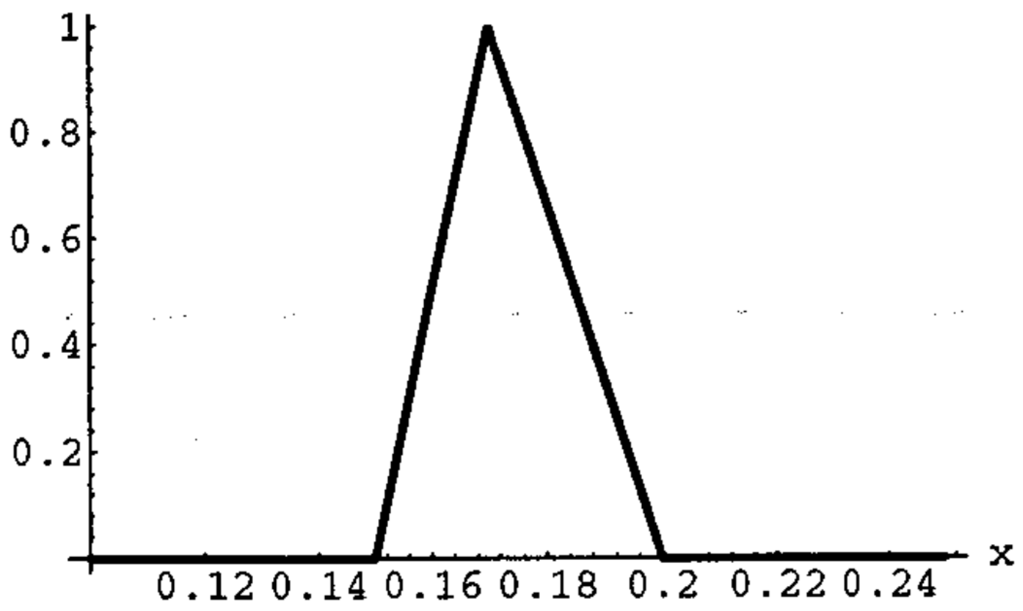
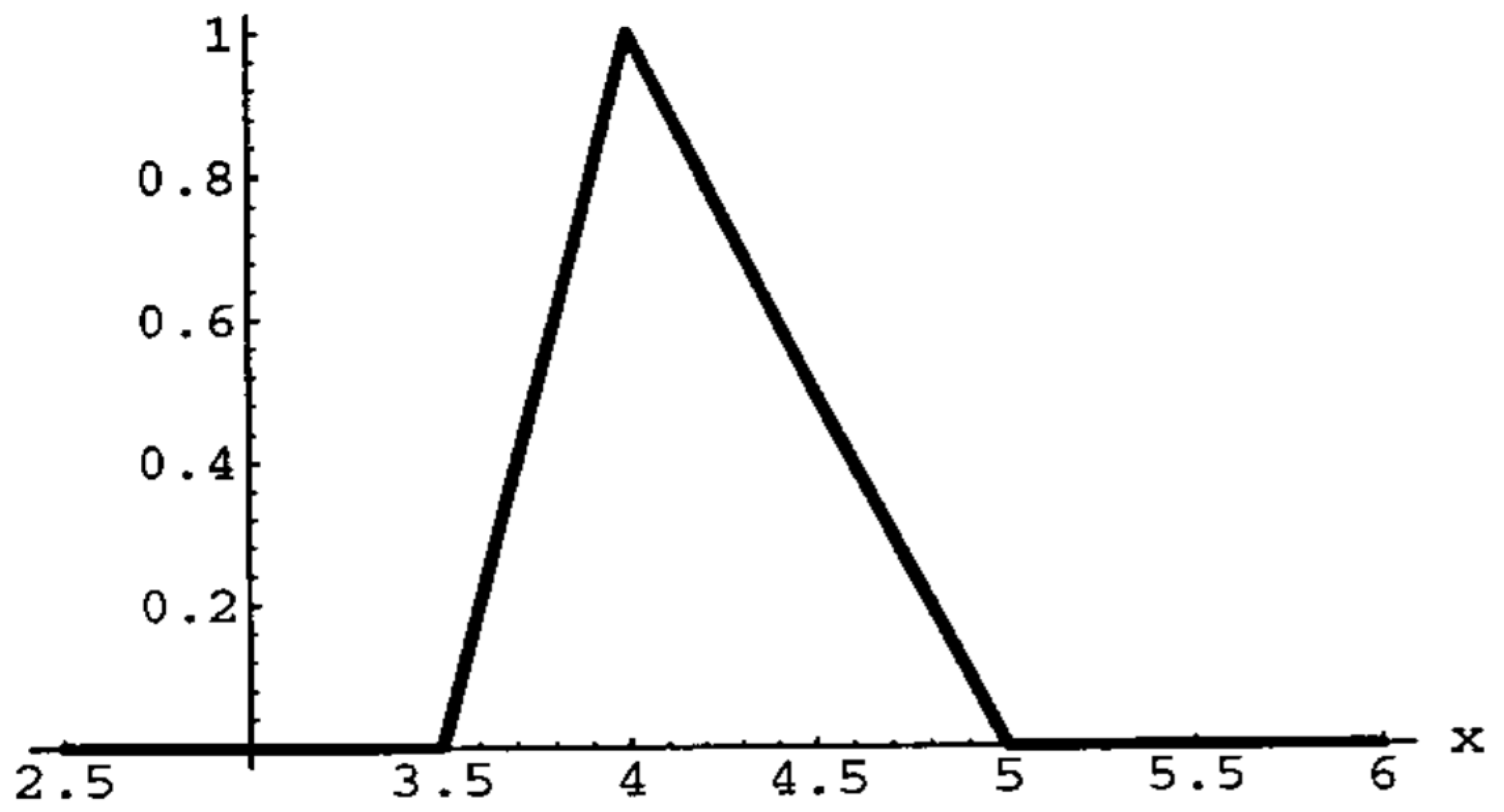
As an illustrative example of the model that we have just developed, we complement the explanation with a specific numerical case, considering $\tilde{a}$ and $\tilde{b}$ as triangular fuzzy numbers with the following values:

$$\tilde{a}=\left(0.15, 0.17, 0.20\right) \tilde{b}=\left(3.5, 4, 5\right)$$

Additionally, considering the initial value for income $Y_0=100$, we will determine the fuzzy values of the guaranteed growth index $\tilde{G}$, as well as income $\widetilde{Y_t}$ and investment $\widetilde{I_t}$ for period t = 4.

In this case, the membership functions of $\tilde{a}$ (marginal propension to save) and $\tilde{b}$ (accelerator) are formed by linear sections, as seen in Figure 1 and Figure 2, respectively.

The analytical expression for the membership function of the fuzzy number $\tilde{a}$ is:

$${\mu }_{\tilde{a}}\left(x\right)=\{\begin{array}{cc}0& if x<0.15\hfill \\ \frac{x-0.15}{0.02}& if 0.15\le x\le 0.17\hfill \\ \frac{0.20-x}{0.03}& if 0.17\le x\le 0.20\hfill \\ 0& if x>0.20\hfill \end{array}$$

The expression of its α-cuts is:

$$a_{\alpha }=\left[0.15+0.02·\alpha , 0.2-0.03·\alpha \right] 0\le \alpha \le 1$$

On the other hand, for the fuzzy number $\tilde{b}$ we have:

$${\mu }_{\tilde{b}}\left(x\right)=\{\begin{array}{cc}0& if x<3.5\hfill \\ \frac{x-3.5}{0.5}& if 3.5\le x\le 4\hfill \\ 5-x& if 4\le x\le 5\hfill \\ 0& if x>5\hfill \end{array}$$

For the expression of its α-cuts it is:

$$b_{\alpha }=\left[3.5+0.5·\alpha , 5-\alpha \right]$$

From the fuzzy equation:

$$\tilde{M}=\frac{\tilde{b}}{\tilde{b}-\tilde{a}}$$

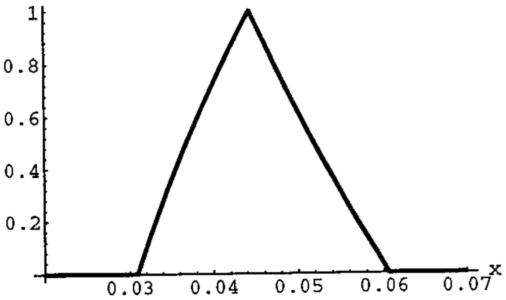
Given the membership functions for ${\mu }_{\tilde{a}}$ and ${\mu }_{\tilde{b}}$, we get the membership function of the fuzzy number $\tilde{M}$ which, as shown in Figure 3, does not correspond to a triangular fuzzy number, because, as we see, this membership function is made up of nonlinear sections. Its expression is given by:

$${\mu }_{\tilde{M}}\left(x\right)=\{\begin{array}{cc}0& if x<1.030\hfill \\ \frac{4.85x-5}{1.02x-1}& if 1.030\le x\le 1.044\hfill \\ \frac{3.5-3.3x}{0.53x-0.5}& if 1.044\le x\le 1.060\hfill \\ 0& if x>1.060\hfill \end{array}$$

From the fuzzy number $\tilde{M}$ we determine the guaranteed growth rate, expressed by means of the fuzzy number $\tilde{G}$, with α-cuts:

$$G_{\alpha }=\left[\frac{0.15+0.02·\alpha }{4.85-1.02·\alpha } , \frac{0.2-0.03·\alpha }{3.3+0.53·\alpha }\right] 0\le \alpha \le 1$$

The membership function ${\mu }_{\tilde{G}}$ takes a similar form to ${\mu }_{\tilde{M}}$ since as we have seen in Equation (51), they are closely related. Its expression is:

$${\mu }_{\tilde{G}}\left(x\right)=\{\begin{array}{cc}0& if x<0.030\hfill \\ \frac{4.85x-0.15}{1.02x+0.02}& if 0.030\le x\le 0.044\hfill \\ \frac{0.2-3.3x}{0.53x+0.03}& if 0.044\le x\le 0.060\hfill \\ 0& if x>0.060\hfill \end{array}$$

As shown in Figure 4, it is not a triangular fuzzy number because it is made up of rational sections.

Finally, we determine the fuzzy expression for income for t = 4, whose α-cuts are:

$$Y_{4\alpha }=\left[{\left(\frac{5-\alpha }{4.85-1.02·\alpha }\right)}^4·100 , {\left(\frac{3.5+0.5·\alpha }{3.3+0.53·\alpha }\right)}^4·100\right]$$

as well as its membership function from Equation (48):

$${\mu }_{\widetilde{Y_4}}\left(x\right)=\{\begin{array}{cc}0& if x<112.55\hfill \\ \frac{1.5337·\sqrt[4]{x}-5}{0.3225·\sqrt[4]{x}-1}& if 112.55\le x\le 118.79\hfill \\ \frac{3.5-1.0435·\sqrt[4]{x}}{0.1676·\sqrt[4]{x}-0.5}& if 118.79\le x\le 126.24\hfill \\ 0& if x>126.24\hfill \end{array}$$

As in all non-triangular membership functions in the example, the coefficients are approximate, but with the degree of accuracy tolerable by the uncertainty situation of the problem.

Finally, to determine the fuzzy expression for investment in period t = 4, we take the uncertain value of the initial investment given by the triangular fuzzy number:

$$\widetilde{I_0}=\left(15,17,20\right) I_{0\alpha }=\left[15+2·\alpha , 20-3·\alpha \right]$$

with which, by application of Equation (56), we determine the α-cuts for investment in period t = 4 which are given by:

$$I_{4\alpha }=\left[{\left(\frac{5-\alpha }{4.85-1.02·\alpha }\right)}^4·\left(15+2·\alpha \right) , {\left(\frac{3.5+0.5·\alpha }{3.3+0.53·\alpha }\right)}^4·\left(20-3·\alpha \right)\right]$$

If we consider the α-cut at level α = 0, we get the support for investment in the considered period:

$$I_{4,0}=\left[\underset{\_}{I_4}\left(0\right), \overline{I_4}\left(0\right)\right]=\left[16.94 , 25.30\right]$$

from which we get the minimum (16.94) and maximum (25.30) estimates for investment in that period.

6. Conclusions

In the paradigm of deterministic models inspired as models of historical construction, these constitute a reflection of the previous behavior at the time of its construction without any possibility to consider sudden changes in the values of the variables due to events not reflected in the historical series. This method of using historical data to make estimates from probability distributions often meets with contradictions in economic reality, which undergoes continual change given the common appearance of new factors not reflected in past behaviors. Therefore, it is convenient, as shown in the present paper, to be able to incorporate in the models future unknown values which can be evaluated by experts with a certain degree of possibility, so that, in this way, models can take into account the continuously changing nature of the economic, social and financial environment. This paper has shown that fuzzy modelling allows introducing inaccuracy by incorporating the variability of model parameters in a reasonable manner. This allows us to obtain a model that includes more information and can therefore produce better future predictions. In this sense, the proposed model allows us to ascertain the impact on the prediction process of income behavior being jointly studied for all possible values of the uncertain parameters considered, each with their own degree of possibility.

Summing up, this paper shows how, by starting with some distributions of possibility for the uncertain magnitudes that are taken as inputs, we can determine the corresponding distribution for any equilibrium values that potentially represent income. Assigning possibility distributions to variables that are not precisely known allows us to provide a proper interpretation of economic reality, thus obtaining forecasts more suited to the real world, since more information is taken into account when applying the model.

On the other hand, from the example based on the classic Harrod’s model of economic growth in the context of uncertainty, we highlight the following points:

1. Under the established fuzzy conditions, that is, considering the marginal propensity to save $\tilde{a}$ and the accelerator $\tilde{b}$ as fuzzy numbers, the results obtained with the application of the model have an interpretation within the context of uncertainty in which they are presented, and, in this sense, they give a more generality to the application of the model, which implies, in this context of uncertainty, a closer approach to reality than the still image that results from the classical application. This study in a fuzzy context allows us to incorporate within the model what would be a broad analysis of sensitivity. The study is a logical generalization because if the parameters that we have considered as fuzzy numbers are reduced to crisp numbers, the results obtained coincide with those resulting from the classical application;

2. When analyzing the behavior of the model under the considered hypotheses of uncertainty, we observe that, as in the context of certainty, income and investment must grow at the same rate to be in equilibrium under the conditions imposed by the model. This rate is given by the growth index, which in this study is expressed as a fuzzy number with the corresponding membership function being expressed from the membership functions ${\mu }_{\tilde{a}}$ and ${\mu }_{\tilde{b}}$;

3. The direct application of the arithmetic of the intervals is not always suitable for the calculation of the fuzzy growth index, since, depending on the form of the expression of this index, the expression of the intervals that determine the α-cuts with the direct application of arithmetic has much more entropy than the calculation of the α-cuts obtained by using the interpretation proposed by Buckley and Qu, which is appropriate in the application of the model presented;

4. If we use $\tilde{G}=1+\tilde{a}/\left(\tilde{b}-\tilde{a}\right)$ as the expression for the growth index, we have found that the applications of the rules of fuzzy arithmetic lead to a correct and interpretable result of the α-cuts of the growth rate. Therefore, by using this expression the usual arithmetic can be applied;

5. As is to be expected, the time factor increases the uncertainty in determining future income and investment values, which is translated into the increase in entropy that characterizes the resulting fuzzy numbers as we move forward in time;

6. The initial value of income $Y_0$, which we consider as a known and therefore crisp, is a value that influences the results only as a scale factor, as in the classical model;

7. From the knowledge of the membership functions ${\mu }_{\tilde{a}}$ and ${\mu }_{\tilde{b}}$, it is possible to determine the membership function for income in any period, and this function adopts a simple and fully operational expression in the case that $\tilde{a}$ and $\tilde{b}$ are triangular fuzzy numbers. On the other hand, for investment values the expression obtained for the membership function is not operational and it is essential in practice to calculate the possible values and their degree of possibility through the expression of their α-cuts;

8. The purpose of the application presented in this paper is how models based on fuzzy numbers work, as well as to analyze how the model behaves when the parameters linked to the variables are fuzzy numbers and need to be operated according to the arithmetic of uncertainty. In further studies it will be necessary to go beyond the simple Harrod model of economic growth and study and analyze models of exogenous and endogenous growth with the aim of building new models based on uncertainty, more suited to the complex economic reality. It should be noted that government expenditure and taxes are not considered in our representation of Harrod’s model. Introducing these variables would prove a fairly straightforward task and would not affect the results produced by the model. An approach that involves exogenous and endogenous growth models would be more interesting, since it would allow us to take into account the role of, for example, technology, education, property rights or human capital, relevant variables missing from the Harrod approach;

9. It should also be noted that our representation of Harrod’s model considers a closed economy and does not take into account the financial aspect of the economy. Nowadays, money flows around the world as countries trade with one another. Indeed, finance was at the heart of the economic crisis before the world was hit by that of the Covid pandemic. Therefore, an interesting approach would be to consider fuzzy logic in a model aimed at the open economy (with imports, exports and financial flows). This would represent a valuable addition to the Mundell–Fleming setting, which takes into account deterministic values for exchange rates, interest rates and output;

10. Beyond the long-term considerations of economic growth, our approach is also useful for analyzing the economy in the short term. By incorporating fuzzy logic, it is possible to study economic fluctuations related to the business cycle. Currently, dynamic stochastic general equilibrium models introduce fluctuations way means of random shocks into the economy. Fuzzy numbers could be used to represent these shocks so that the model takes into account the uncertainty pervading the real world;

11. Finally, considering macroeconomic variables as fuzzy numbers may also represent a way of improving the current measurements used by traditional economic models. It is well known that real world measures of national income, consumption, saving, investment, exports or imports are subject to uncertainty. Indeed, national accounts data are subject to frequent revisions as new information emerges. Presenting macroeconomic variables as fuzzy numbers would make the uncertainty inherent in such magnitudes apparent and result in policymakers being able to make more informed decisions.

Consequently, the modeling presented in this article expands the possibilities offered by the current Harrod’s growth model [29,30,31], and continues along the path first followed with the proposal to use fuzzy numbers [11,12].

References

- Solow, R.M. A contribution to the theory of economic growth. Q. J. Econ. 1956, 70, 65–94. [Google Scholar] [CrossRef]
- Zadeh, L.A. Fuzzy Sets. Inf. Control 1965, 8, 338–353. [Google Scholar] [CrossRef] [Green Version]
- Zadeh, L.A. Fuzzy Sets as a basis for a theory of possibility. Fuzzy Sets Syst. 1978, 1, 3–28. [Google Scholar] [CrossRef]
- Ferrer-Comalat, J.C.; Linares-Mustarós, S.; Corominas-Coll, D. A formalization of the theory of expertons. Theoretical foundations, properties and development of software for its calculation. Fuzzy Econ. Rev. 2016, 21, 23–39. [Google Scholar] [CrossRef]
- Ferrer-Comalat, J.C.; Linares-Mustarós, S.; Corominas-Coll, D. A generalization of the theory of expertons. Int. J. Uncertain. Fuzziness Knowl. Based Syst. 2018, 26 (Suppl. 1), 121–139. [Google Scholar] [CrossRef]
- Linares-Mustarós, S.; Ferrer-Comalat, J.C.; Corominas-Coll, D.; Merigó, J.M. The ordered weighted average in the theory of expertons. Int. J. Intell. Syst. 2019, 34, 345–365. [Google Scholar] [CrossRef]
- Linares-Mustarós, S.; Ferrer-Comalat, J.C.; Corominas-Coll, D.; Merigó, J.M. The weighted average multiexperton. Inf. Sci. 2021, 557, 355–372. [Google Scholar] [CrossRef]
- Billot, A. Economic Theory of Fuzzy Equilibria; Springer: Berlin, Germany, 1992. [Google Scholar]
- Mansur, Y. Fuzzy Sets and Economics; Edward Elgar Publishing: Cheltenham, UK, 1995. [Google Scholar]
- Ponsard, C. Fuzzy mathematical models in economics. Fuzzy Sets Syst. 1988, 28, 273–283. [Google Scholar] [CrossRef]
- Ferrer-Comalat, J.C.; Linares-Mustarós, S.; Corominas-Coll, D. Fuzzy logic in economic models. J. Intell. Fuzzy Syst. 2020, 38, 5333–5342. [Google Scholar] [CrossRef]
- Ferrer-Comalat, J.C.; Linares-Mustarós, S.; Corominas-Coll, D. A Fuzzy Economic Dynamic Model. Mathematics 2021, 9, 826. [Google Scholar] [CrossRef]
- Easterly, W. Ghost of the Financing Gap: How the Harrod-Domar Model Still Haunts Development Economics; World Bank Development Research Group: Washington, DC, USA, 1997. [Google Scholar]
- Solow, R.M. Perspectives on Growth Theory. J. Econ. Perspect. 1994, 8, 45–54. [Google Scholar] [CrossRef] [Green Version]
- Swan, T.W. Economic growth and capital accumulation. Econ. Rec. 1956, 32, 334–361. [Google Scholar] [CrossRef]
- Romer, P.M. The Origins of Endogenous Growth. J. Econ. Perspect. 1994, 8, 3–22. [Google Scholar] [CrossRef] [Green Version]
- Kosko, B. Fuzzy Thinking: The New Science of Fuzzy Logic; Hyperion: New York, NY, USA, 1993. [Google Scholar]
- Linares Mustarós, S.; Viladevall Valldeperas, Q.; Llacay Pintat, T.; Ferrer-Comalat, J.C. An introduction to the foundations of fuzzy logic through art. CUAd C 2018, 20, 133–156. [Google Scholar]
- Zadeh, L.A. Similarity relations and fuzzy orderings. Inf. Sci. 1971, 3, 177–200. [Google Scholar] [CrossRef]
- Zadeh, L.A.; Fu, K.S.; Tanaka, K.; Shimura, M. Fuzzy Sets and Their Applications to Cognitive and Decision Processes; Academic Press: New York, NY, USA, 1975. [Google Scholar]
- Jain, R. Tolerance analysis using fuzzy sets. Int. J. Syst. Sci. 1976, 7, 1393–1401. [Google Scholar] [CrossRef]
- Dubois, D.; Prade, H. Fuzzy Sets and Systems: Theory and Applications; Academic Press: New York, NY, USA, 1980. [Google Scholar]
- Zimmerman, H.J. Fuzzy Set Theory and Its Applications; Kluwer Academic Publishers: Boston, FL, USA, 2000. [Google Scholar]
- Nguyen, H.T. A note on the extensions principle for fuzzy sets. J. Math. Anal. Appl. 1978, 64, 369–380. [Google Scholar] [CrossRef] [Green Version]
- Buckley, J.J. On using α-cuts to evaluate fuzzy equations. Fuzzy Sets Syst. 1990, 38, 309–312. [Google Scholar] [CrossRef]
- Moore, R. Methods and Applications of Interval Analysis; SIAM: Philadelphia, PA, USA, 1979. [Google Scholar]
- Buckley, J.J.; Qu, Y. Solving fuzzy equations: A new solution concept. Fuzzy Sets Syst. 1991, 39, 291–301. [Google Scholar] [CrossRef]
- Keynes, J.M. The General Theory of Employment, Interest, and Money; Springer: Berlin, Germany, 2018. [Google Scholar]
- Harrod, R.F. An essay in dynamic theory. Econ. J. 1939, 49, 14–33. [Google Scholar] [CrossRef]
- Domar, E.D. Capital expansion, rate of growth, and employment. Econom. J. Econom. Soc. 1946, 14, 137–147. [Google Scholar] [CrossRef]
- Domar, E.D. Expansion and employment. Am. Econ. Rev. 1947, 37, 34–55. [Google Scholar]
Figure 1.
Membership function of marginal propension to save (mps).
Figure 2.
Membership function for the accelerator.
Figure 3.
Membership function for .
Figure 4.
Membership function for the growth index.