Degree Reduction of Q-Bézier Curves via Squirrel Search Algorithm

Abstract

Q-Bézier curves find extensive applications in shape design owing to their excellent geometric properties and good shape adjustability. In this article, a new method for the multiple-degree reduction of Q-Bézier curves by incorporating the swarm intelligence-based squirrel search algorithm (SSA) is proposed. We formulate the degree reduction as an optimization problem, in which the objective function is defined as the distance between the original curve and the approximate curve. By using the squirrel search algorithm, we search within a reasonable range for the optimal set of control points of the approximate curve to minimize the objective function. As a result, the optimal approximating Q-Bézier curve of lower degree can be found. The feasibility of the method is verified by several examples, which show that the method is easy to implement, and good degree reduction effect can be achieved using it.

1. Introduction

In the representation of a curve or surface, it is crucial which bases are used if the shape and characteristics of the curve or surface are wished to be preserved. CAGD/CAD Bézier curves and surfaces are among the most prevalent in the shape design of multiple products owing to their many excellent properties, including end-points properties, symmetry, linear, convex hull property, variation diminishing property, recurrence properties, and simple integral and derivative formulas [1]. However, given a set of control points, the Bézier curve can be constructed. If the shape of a Bézier curve needs to be adjusted, the designer has to modify its control points, which makes the design operation cumbersome and inconvenient to be applied in practical engineering applications and design.

For addressing this defect, scholars proposed rational Bézier curves by introducing weighted factors by which its shape can be adjusted by fixing the control points and by changing the weighted factors. But this newly invented Bézier curve with rational factor generates some computational complexity, complex integration, and multiple derivations, as [2,3].

In order to maintain the excellent properties of the Bézier model and to enhance its shape adjustability, and improve its approximation effect to curves of real world, numerous non-rational Bézier curves with shape parameters are proposed and used for constructing different types of surfaces, e.g., SG-Bézier [4,5,6], H-Bézier [7,8], T-Bézier [9,10], and the following Q-Bézier curves [11,12,13], etc. Without changing control points, the shape of these generalized Bézier curves can be adjusted flexibly by modifying their shape parameters. In 1997, Phillips [11] first proposed Q-Bernstein polynomials, which generalize the classical Bernstein polynomials. Based on the Q-Bernstein polynomials, Oruc and Phillips [12] defined the Q-Bernstein basis functions and further defined the Q-Bézier curves associated with the shape parameter q. Q-Bézier curves share many excellent properties with classic Bézier curves, e.g., non-negativity, partition of unity, convex hull property, end-points properties, variation diminishing property, etc. The introduction of the shape parameter q significantly enhances the shape adjustability of Q-Bézier curves. Based on the De Casteljau algorithm, Disibuyuk and Oruc [13] proposed rational Q-Bézier curves. Simeonov et al. [14] deduced a recursive evaluation algorithm and an explicit subdivision procedure for Q-Bézier curves. Goldman et al. [15] derived explicit formulas for the generating functions of the Q-Bernstein basis functions in terms of q-exponential functions and proved a variety of identities for the Q-Bernstein bases. Han et al. [16] constructed a new Lupaş q-Bézier model by using Lupaş q-analogue Bernstein operator. Furthermore, Han et al. proposed a weighted Lupaş q-Bézier curve and studied its degree evaluation and De Casteljau’s algorithms in [17]. Liu et al. [18] provided some remarks on the Q-Bézier curves constructed by [17] and revisited the rational quadratic case of the curves. Hu et al. [19] derived G¹ and G² continuity conditions of adjacent (m, n)-degree Q-Bézier surfaces with shape parameters. Jegdić et al. [20] defined a (q, h)-blossom operator of bivariate Bernstein polynomials, and presented the corresponding rectangular tensor product (q, h)-Bézier surfaces. Recently, Delgado [21] investigated the geometric properties and algorithms for rational Q-Bézier curves and surfaces. In spite of so many works on Q-Bézier curves, the multiple-degree reduction of Q-Bézier curves are rarely studied.

Degree reduction problem of curves was firstly presented as the inverse problem of degree elevation. The problem of degree reduction of curves is to approximate an original curve with another curve of lower degree. In actual operation, different CAD/CAM systems usually have different demands for the degree of curves. Thus, for data conversation and transmission between various models, we properly investigated the degree reduction/elevation of curves. For the degree reduction of curves, the three methods were proposed based on the least square theory [22,23,24,25], the algebraic method [26,27,28,29,30], and the intelligent optimization algorithm based methods, in which the problem of degree reduction is formulated as an optimization one and is solved by incorporating intelligent optimization algorithms [31,32,33,34]. In 2019, based on the genetic simulated annealing algorithm, Lu and Qin [31] realized the multi-degree reduction approximation of the S-λ curve for the first time. Hu et al. [32] studied the problem of approximate multi-degree reduction for SG-Bézier curves using the grey wolf optimizer algorithm, and achieved a good degree reduction effect. After that, Qin et al. [33] further extended the method in literature [32] to the degree reduction of SG-Bézier surfaces. Guo et al. [33] improved the whale optimization algorithm by using the skewed normal cloud and applied it to solve the problem of degree reduction for S-λ curve. Compared with the first two methods, the third kind of method in [31,32,33,34] is more convenient to be used for the multiple-degree reduction of different types of curves. Moreover, these methods based on intelligent optimization algorithms seem simpler, by which global optimal degree reduced curves can be obtained intelligently, avoiding complicated theoretical derivation.

It is difficult to solve the problem of degree reduction for the Q-Bézier curves by the traditional method, but the degree reduction of Q-Bézier curves is, mathematically, an optimization problem that can be effectively solved by swarm intelligence algorithm (SIA). SIA accomplishes the corresponding algorithm by simulating the collective behaviors of various biological groups in nature, and it has the merits of easy realization, high computational efficiency, and wide application [35]. As we all know, the most famous SIA is particle swarm optimization (PSO) presented by Kennedy and Eberhart [36] in 1995, but PSO itself has some shortcomings. In recent years, grey wolf optimization algorithm (GWO) [37], whale optimization algorithm (WOA) [38], salp swarm algorithm (SSA) [39], grasshopper optimization algorithm (GOA) [40], Harris Hawks optimization (HHO) [41], squirrel search algorithm (SSA) [42], and some other SIA have emerged one after another. Among them, the SSA with higher solving accuracy and better performance was presented by Jain et al. [42] in 2019. Since then, the SSA has been well applied in many practical fields [43,44]. Due to the extensive application of Q-Bézier curves and the significant function that degree reduction plays in data conversion between different CAD/CAM systems, as well as the superiorities and potential possessed by intelligent optimizers in solving optimization problems, this paper propose a new method for the degree reduction of Q-Bézier by incorporating the high-efficient swarm intelligence-based squirrel search algorithm.

The outline of this paper is as follows. In Section 2 and Section 3, Q-Bézier curves and squirrel search algorithm are described, respectively. Section 4 presents the multiple-degree reduction of Q-Bézier curves via squirrel search algorithm. Experimental results are given in Section 5, and for a brief summary of the paper, see Section 6.

2. The Definition of Q-Bézier Curves

Definition 1.

The n degree Q-Bernstein polynomials basis functions are defined as follows [12]

$$L_{k,n}(\eta )=\left(\begin{array}{c}n\\ k\end{array}\right){\eta }^k{\displaystyle \prod _{j=0}^{n-k-1}(1-q^k\eta )},0\le k\le n$$

(1)

Remark 1.

For any$q\in (0,1]$, the Q-Bernstein polynomials basis functions defined by (1) are non-negative in$\eta \in [0,1]$. With q = 1, the Q-Bernstein polynomials basis functions become the classic Bernstein polynomials basis functions.

Remark 2.

Q-Bernstein polynomials basis functions defined by (1) can be re-presented as the following form:

$$L_{k,n}(\eta )={\displaystyle \sum _{p=k}^n{(-1)}^{p-k}}{q}^{(p-k)(p-k-1)/2}\left(\begin{array}{c}n\\ p\end{array}\right)\left(\begin{array}{c}p\\ k\end{array}\right){\eta }^p$$

(2)

Definition 2.

Given a set of control points$T_k\in R^z,\forall z=2,3,(k=0,1,\dots ,n)$, the curve

$$y(\eta )={\displaystyle \sum _{k=0}^n{T}_k}{L}_{k,n}(\eta ),0\le \eta \le 1,$$

(3)

is called the Q-Bézier curve of degree n with a shape parameter q [12], where $L_{k,n}(\eta )$ is the Q-Bernstein polynomials basis function defined in (1). The Q-Bézier curve becomes classic Bézier curve with q = 1.

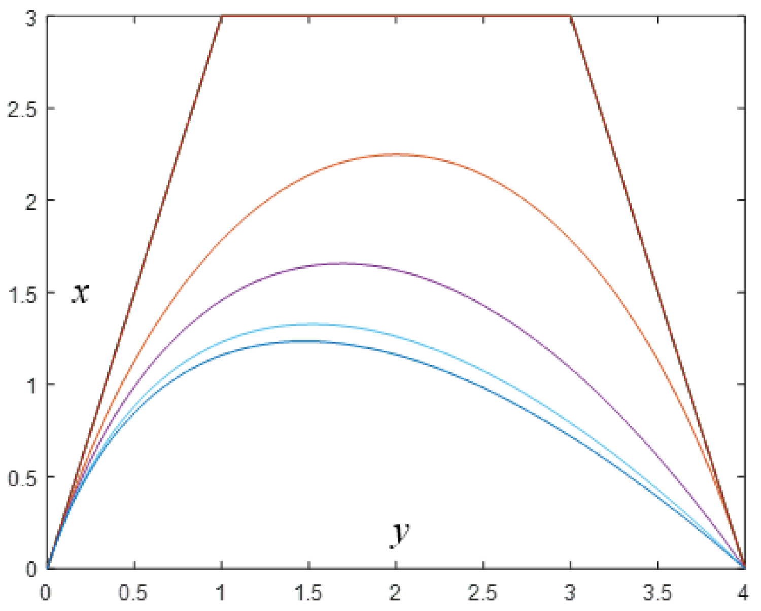
For classic Bézier curves, their shapes are obtained by using the control points. But for Q-Bézier curves, their shapes can be adjusted expediently by modifying the shape parameter q while keeping their control points unchanged. Figure 1 gives an example to illustrate the shape modification effect of the shape parameter q. As can be seen from Figure 1, with the increase of q, the curve moves towards its control polygon.

3. Squirrel Search Algorithm (SSA)

3.1. The Basic Principles of Squirrel Search Algorithm

The squirrel search algorithm was proposed in 2019. The idea of this algorithm was inspired by the dynamic behavior of squirrels to search out the food and their active flying movement, which are modelled mathematically for the SSA optimization technique. This algorithm is claimed to be effective in the optimization of complicated multidimensional problems with simple principles, handy calculations and reliable results. Ever since its proposal, the squirrel search algorithm has been used in the field of wireless sensor networks [43], brain tumor detection [44], etc. The basic rule of the squirrel search algorithm is as follows.

In order to simplify the SSA optimization technique, the following steps are to be followed:

(1)

Suppose that the forest contains n flying squirrels and there is only one squirrel on the tree.

(2)

Each flying squirrel hunted for food by its own for the progress of the algorithm.

(3)

In the forest, there are eucalyptus trees, bananas tree and normal trees.

(4)

Suppose the forest contains one eucalyptus tree, three banana trees and the other trees are all normal trees.

(5)

If the squirrels do not find the food to survive then they will move to other positions for hunting.

3.2. Implementation of Squirrel Search Algorithm (SSA)

Similar to other population-based algorithms, SSA starts from a random initial position of the flying squirrels. In the d-dimensional search space, the position of a flying squirrel is represented by a vector. The implementation steps of squirrel search algorithm are as follows [42].

Step 1.

Initial stage: suppose there are n squirrels in the forest, each of whose position can be represented by a vector. The positions of the entire swarm $FG$ is given in the below matrix form:

$$FG=\left[\begin{array}{cccc}F{G}_{1,1}& F{G}_{1,2}& \cdots & F{G}_{1,d}\\ F{G}_{2,1}& F{G}_{2,2}& \cdots & F{G}_{2,d}\\ ⋮& ⋮& \ddots & ⋮\\ F{G}_{n,1}& F{G}_{n,2}& \cdots & F{G}_{n,d}\end{array}\right]$$

where $F{G}_{k,j}$ denotes the jth dimension of kth flying squirrel.

In initialized steps, if we want to make a uniform search and each swarm started at a random position in the solution space, that is

$$F{G}_{k,j}=F{G}_L+U(0,1)\times (F{G}_U-F{G}_L)$$

(4)

where U(0, 1) is any unspecified number from domain [0,1] and $F{G}_L$ and $F{G}_U$ denotes the lower and upper bounds respectively in jth dimension.

Step 2.

Fitness evaluation: for evaluating the goodness of the position of each flying squirrel. We may choose a variable and put it into a specified fitness function and then arrange these values as follows:

$$F=\left[\begin{array}{c}f([F{G}_{1,1},F{G}_{1,2},\cdots ,F{G}_{1,d}])\\ f([F{G}_{2,1},F{G}_{2,2},\cdots ,F{G}_{2,d}])\\ ⋮\\ f([F{G}_{n,1},F{G}_{n,2},\cdots ,F{G}_{n,d}])\end{array}\right]$$

where f () is the fitness function.

Step 3.

Finding, declaration, and random selection: in the initial step, we may arrange the fitness values in ascending order. The flying squirrel with the smallest fitness value is assumed to be on the eucalyptus tree. The next three flying squirrels are assumed to be on the banana trees and they are assumed to move towards the eucalyptus tree. The remaining flying squirrels are supposed to be on the normal trees. Some of them are assumed to move toward the eucalyptus tree while the others are assumed to move toward the banana trees. The flying squirrels are affected only by the predators similarly to other swarm intelligence-based algorithms which are modelled by resorting to a predator presence probability ($P_{dp}^{}$).

Step 4.

Position updating: the three aforementioned situations in Step 3 which occur during the hunting of the flying squirrels can be mathematically modelled as follows:

Case 1.

When squirrels on banana trees ($F{G}_{a\eta }^{\eta }$) move toward the eucalyptus tree, their new positions can be mathematically written as follows:

$$F{G}_{a\eta }^{\eta +1}=\left\{\begin{array}{cc}F{G}_{a\eta }^{\eta }+d_g\times M_c\times (F{G}_{h\eta }^{\eta }-F{G}_{a\eta }^{\eta }),& R_1\ge P_{dp}\\ Randomlocation,& Otherwise\end{array}\right.$$

(5)

where $R_1$ is a random number in [0, 1], $F{G}_{h\eta }^{\eta }$ represents the place of the flying squirrel on the eucalyptus tree. $M_c$ is a gliding constant, which is assumed to be 1.9 here. $d_g$ is the distance defined according to the aerodynamics of gliding. A random gliding distance $d_g$ can be generated by incorporating a random variation in lift coefficient C_L in the range 0.675 ≤ C_L ≤ 1.5 in (6)

$$d_g=(\frac{h_g}{\tan \varphi }),$$

(6)

where

$$\varphi =\arctan (\frac{D}{L})=\arctan (\frac{1/2\rho C_L{V}^{2}S}{1/2\rho C_D{V}^{2}S})=\arctan (\frac{C_L}{C_D}).$$

Here $\varphi$ refers to the glide angle, D and L are lift and drag forces, respectively, $(\rho =1.204kg{m}^{-3})$ is the density of the air, $(V=5.25m{s}^{-1})$ is speed, (S = 154 cm ²) is the surface area of the body, (h_g = 9 m) is the mislaying height occurred due to gliding. C_D is frictional drag coefficient, which is considered to be fixed at 0.60 here. C_L is the lift coefficient.

Case 2.

Some of the flying squirrels on normal trees ($F{G}_{n\eta }$) may move toward banana trees for food and their new positions can be seen as follows:

$$F{G}_{n\eta }^{\eta +1}=\left\{\begin{array}{cc}F{G}_{n\eta }^{\eta }+d_g\times G_c\times (F{G}_{a\eta }^{\eta }-F{G}_{n\eta }^{\eta }),& R_2\ge P_{dp},\\ Randomlocation,& otherwise,\end{array}\right.$$

(7)

where $R_2$ is an arbitrary number in [0,1].

Case 3.

When other flying squirrels on normal trees ($F{G}_{n\eta }$) will move toward the eucalyptus tree for food, their new positions can be represented as

$$F{G}_{n\eta }^{\eta +1}=\left\{\begin{array}{cc}F{G}_{n\eta }^{\eta }+d_g\times G_c\times (F{G}_{h\eta }^{\eta }-F{G}_{n\eta }^{\eta }),& R_3\ge P_{dp},\\ Randomlocation,& otherwise,\end{array}\right.$$

(8)

where $R_3$ is an arbitrary number in [0, 1].

In these cases, the value of predator presence probability $P_{dp}^{}$ is set to be 0.1.

Step 5.

Seasonal monitoring condition checking:

• Calculate seasonal constant ($G_c^{\eta }$).

  $$G_c^{\eta }=\sqrt{{\displaystyle \sum _{k=1}^d(F{G}_{a\eta ,j}^{\eta }-F{G}_{h\eta ,j})}}$$

  (9)
• Check the seasonal monitoring condition i.e., ($G_c^{\eta }<G_{\min }$), where Gmin represent the smallest value of seasonal constant can be found as follows:

  $$G_{\min }=\frac{10E^{-6}}{{(365)}^{\eta /({\eta }_m/2.5)}},$$

  (10)

  where $\eta$ and ${\eta }_m$ represents iteration values.
• If $G_c^{\eta }<G_{\min }$ then again consider the flying squirrels without food on eucalyptus tree by (11).

  $$F{G}_{n\eta }^{new}=F{G}_L+Levy(n)\times (F{G}_U-F{G}_L)$$

  (11)

  where Lévy distribution in [45] can be applied for better result.

Step 6.

Repeation: if you do not meet to the desired criteria then repeat Step 2 and set the optimal parameter to get the desired result.

4. Degree Reduction of Q-Bézier Curves with the Grey Wolf Optimizer

4.1. The Problem of Degree Reduction of Q-Bézier Curve

A Q-Bézier curve of degree n with control points ${\left\{T_k\right\}}_{k=0}^n$, is defined as

$$y(\eta )={\displaystyle \sum _{k=0}^n{T}_k}{L}_{k,n}(\eta ),$$

(12)

the so-called degree reduction means selecting the set of control points ${\left\{H_j\right\}}_{j=0}^m$ such that the corresponding low-mth-degree Q-Bézier curve

$$z(\eta )={\displaystyle \sum _{j=0}^m{H}_j}{L}_{j,m}(\eta ),$$

(13)

meets the condition

$$\underset{0\le \eta \le 1}{\max }d(y(\eta ),z(\eta ))=\underset{0\le \eta \le 1}{\max }||y(\eta )-z(\eta )|{|}_2=\min$$

(14)

With this optimization problem the degree reduction of the Q-Bézier curve can be formulated as follows:

$$\begin{gathered} f(y,z,\eta ;q)=\underset{0\le \eta \le 1}{\min \max }d(y(\eta ),z(\eta )) \\ \mathrm{s}.\mathrm{t}.{\left\{T_k\right\}}_{k=0}^n{\left\{H_j\right\}}_{j=0}^m\in R^d,\eta \in [0,1];0<q\le 1, \end{gathered}$$

(15)

where T and H are the control points of the Q-Bézier curve before and after the degree reduction, q is the shape parameter of Q-Bézier curve.

Due to the complexity of degree reduction of curves by traditional methods and the superiorities and potential possessed by swarm intelligence-based optimization techniques in addressing complex optimization problems, we resorted to the squirrel search algorithm to solve the degree reduction problem for its many aforementioned advantages. The degree reduction algorithm of Q-Bézier curve via squirrel search algorithm can be described as follows.

4.2. Initialization of the Flying Squirrel Population

The degree reduction algorithm of Q-Bézier curves starts with a random initialized population, which is composed of a group of feasible control points sequences of the Q-Bézier curve after degree reduction. The initial positions of the population within the provided feasible range [T_min, T_max] can be generated by

H_j = T_min+ α_j(T_max −T_min), j = 0, 1,..., m,

(16)

where x_min and x_max are, respectively, the smallest and largest values of x-component of control points ${\left\{T_k\right\}}_{k=0}^n$, y_min and y_max are, respectively, the smallest and largest values of y-component of control points ${\left\{T_k\right\}}_{k=0}^n$. T_min = (x_min, y_min), T_max = (x_max, y_max). α_j is a random number in [0,1].

Additionally, if the end points of the original Q-Bézier need to be retained, we take

H₀ = T₀, H_m = T_n.

(17)

4.3. Selection of Fitness Function

For achieving a good approximation effect after degree reduction, it is necessary to define a distance function, namely the objective function or fitness function in optimization, to measure how close the degree reduced Q-Bézier curve is to the original Q-Bézier curve. Here, the fitness function is defined as:

$$f(y,z)=\underset{0\le \eta \le 1}{\max }||y(\eta )-z(\eta )|{|}^2=\underset{k=0}{\overset{s}{\max }}||y({\eta }_k)-z({\eta }_k)|{|}^2,$$

(18)

where $d(y({\eta }_k),z({\eta }_k))$ is the Euclidean distance, ${\left\{{\eta }_j\right\}}_{j=0}^s$ are evenly distributed in [0, 1].

4.4. The Algorithm Description for Degree Reduction of Q-Bézier Curve

In the proposed method, the position of each flying squirrel is defined as a sequence of control points of the approximating degree reduced Q-Bézier curve. The constant updating of the positions of the flying squirrels implies the continuous improvement of the group of solutions, i.e., the group of degree reduced curves, which is the main strength of the method. On the basis of the aforementioned squirrel search algorithm (SSA), the steps to the degree reduction of Q-Bézier curves are described in Algorithm 1, and the corresponding pseudo code is provided in Algorithm 2.

Algorithm 1 Squirrel search algorithm: steps to SSA-based degree reduction of Q-Bézier curve.

Step 1: Specify the number of control points of the degree reduced Q-Bézier curve after input of the original Q-Bézier curve {T0, T1, …, Tn}. Step 2: The adjustable parameters of SSA (flock size, the maximum number of iterations M, predator presence probability ($P_{dp}^{}$) are valued and an optimal value range for each decision is provided which helps us to find the solution. Additionally, the sampling parameter values used for measuring the distance between two curves should be specified. Step 3: Initialize the positions of the population Hj (j = 0, 1, …, m) by (16). Step 4: Evaluate the fitness of each flying squirrel by (18) and store their positions in an array in ascending order of fitness value. Step 5: Update the position of the flying squirrels in the population by (5–8). Step 6: Check the seasonal monitoring condition by (9–10): if the condition is fulfilled, then consider those flying squirrels which are not on the eucalyptus tree by (11). Step 7: Check the termination condition: if the termination condition is fulfilled, execute. Step 8: Otherwise, go back to Step 4. Step 8: Output the set of optimal decision variables, which is just the optimal sequence of control points for the degree reduced Q-Bézier curve. Step 9: Output the optimal degree-reduced Q-Bézier curve and show its approximation effect to the original Q-Bézier curve.

Algorithm 2 The pseudo code of SSA-based degree reduction of Q-Bézier curves

Begin: Define the input parameters. Initialize the positions (sequences of control points) of n flying squirrel randomly by (16). Evaluate the fitness of each sequence of control points (i.e., flying squirrel’s position) by (18). Find the position of the squirrels in increasing order. Determine the flying squirrels on the eucalyptus tree, banana trees and the normal trees, and their intended moving direction based on the aforementioned assumption. while (the termination condition not fulfilled) for m = 1 to $n_1$ ($n_1$ denotes squirrels on banana trees). $$\begin{array}{l}If{R}_1>P_{dp}\\ F{G}_{a\eta }^{\eta +1}=F{G}_{a\eta }^{\eta }+d_g\times G_c\times (F{G}_{h\eta }^{\eta }-F{G}_{a\eta }^{\eta })\\ else\\ F{G}_{a\eta }^{\eta +1}=anunspecifiedposition\\ end\end{array}$$ for m = 1 to $n_2$ ($n_2$ denotes flying squirrels on normal trees and moving to the banana trees). $$\begin{array}{l}If{R}_2>P_{dp}\\ F{G}_{n\eta }^{\eta +1}=F{G}_{n\eta }^{\eta }+d_g\times G_c\times (F{G}_{a\eta }^{\eta }-F{G}_{n\eta }^{\eta })\\ else\\ F{G}_{a\eta }^{\eta +1}=anunspecifiedposition\\ end\end{array}$$ for m = 1 to $n_3$ ($n_3$ denotes squirrels on normal trees and moving to the eucalyptus tree). $$\begin{array}{l}If{R}_3>P_{dp}\\ F{G}_{n\eta }^{\eta +1}=F{G}_{n\eta }^{\eta }+d_g\times G_c\times (F{G}_{a\eta }^{\eta }-F{G}_{n\eta }^{\eta })\\ else\\ F{G}_{a\eta }^{\eta +1}=anunspecifiedposition\\ end\end{array}$$ end Executed the operations 3, 4, 5 sequentially. Compute the seasonal constant $G_c^{\eta }$ by (9),   if (season checking criterion is fulfilled)     choose the unspecific squirrels as in (11)   end     Update the smallest value of constant ($G_{\min }$) by (10) end Output the position of the squirrel with the minimum fitness value in the population, which is the final optimal sequence of control points for the degree reduced Q-Bézier curve. End

5. Examples of Approximate Degree Reduced Q-Bézier Curves

Extensive numerical experiments are given in this section to check the effectiveness of the proposed method. The proposed algorithm has been implemented with MATLAB platform. All experiments are performed on a laptop with E54002.7Ghz CPU and RAM4GB memory. Consider the PS of squirrels as 20 and the iterations are 300. The L₂-norm is used to measure the distance between two parametric curves. In this paper, an error function of degree reduction [46]

$$\epsilon =d_{L_2}(y(\eta ),z(\eta ))={\displaystyle \underset{0}{\overset{1}{\int }}\left|\right|y(\eta )-z(\eta )|{|}^2}d\eta$$

(19)

is used to find the approximation effect between the degree reduced Q-Bézier curves and the original Q-Bézier curves.

5.1. Examples of One-Degree Reduction of Q-Bézier Curves

Example 1.

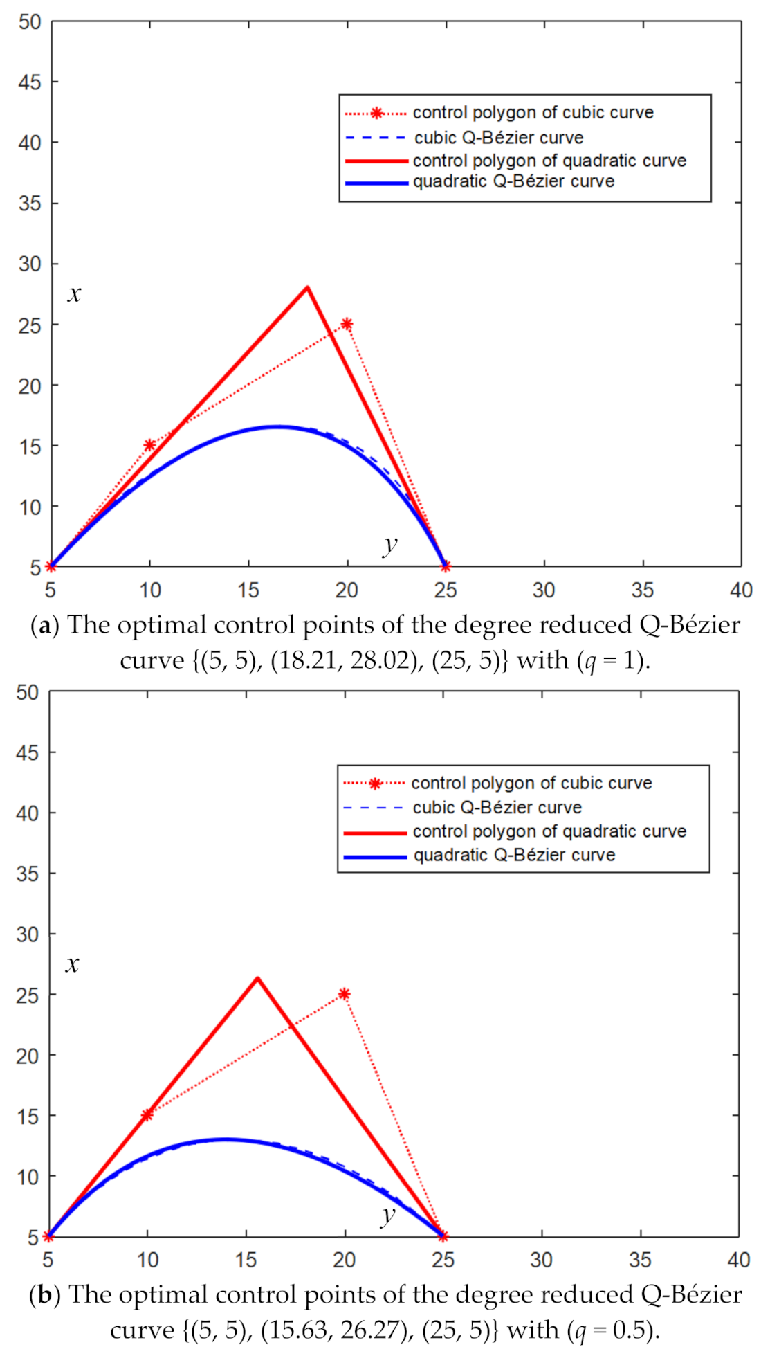
Given the control points of a cubic Q-Bézier curve {T₀ = (0, 20), T₁ = (5, 25), T₂ = (8, 5), T₃ = (15, 20), T₄ = (20, 20), T₅ = (30, 5), T₆ = (40, 15)}, the generated cubic Q-Bézier curve (blue dot line) and the approximating quadratic Q-Bézier curve (blue solid line) are shown in Figure 2a with q = 1. Another pair of curves with q = 0.5 are shown in Figure 2b.

Example 2.

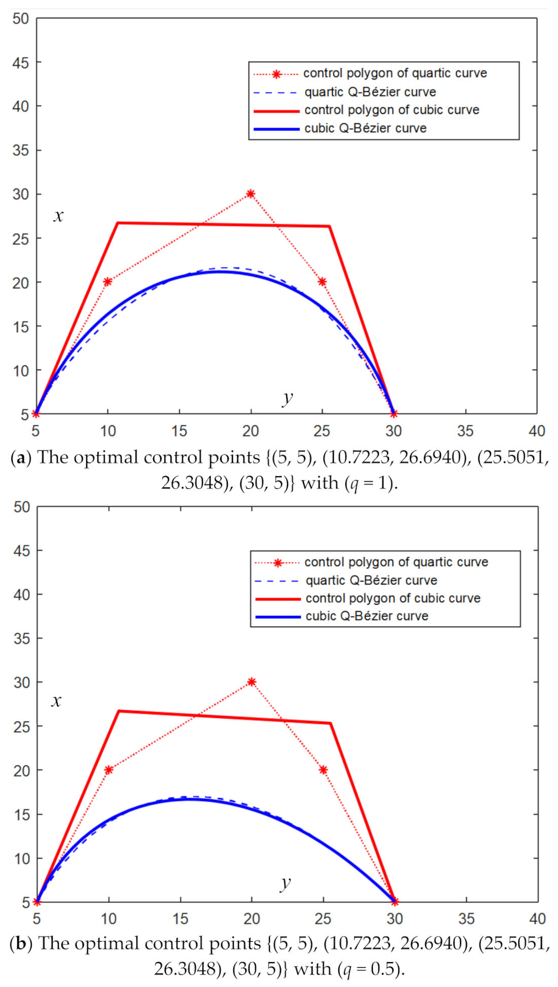
Given the control points of a quartic Q-Bézier curve {T₀ = (5, 5), T₁ = (10, 20), T₂ = (20, 30), T₃ = (25, 20), T₄ = (30, 5)}, the generated quartic Q-Bézier curve (blue dot line) and the approximating cubic Q-Bézier curve (blue solid line) are shown in Figure 3a with q = 1. Another pair of curves with q = 0.5 are shown in Figure 3b.

5.2. Examples of Multiple-Degree Reduction of Q-Bézier Curves

Example 3.

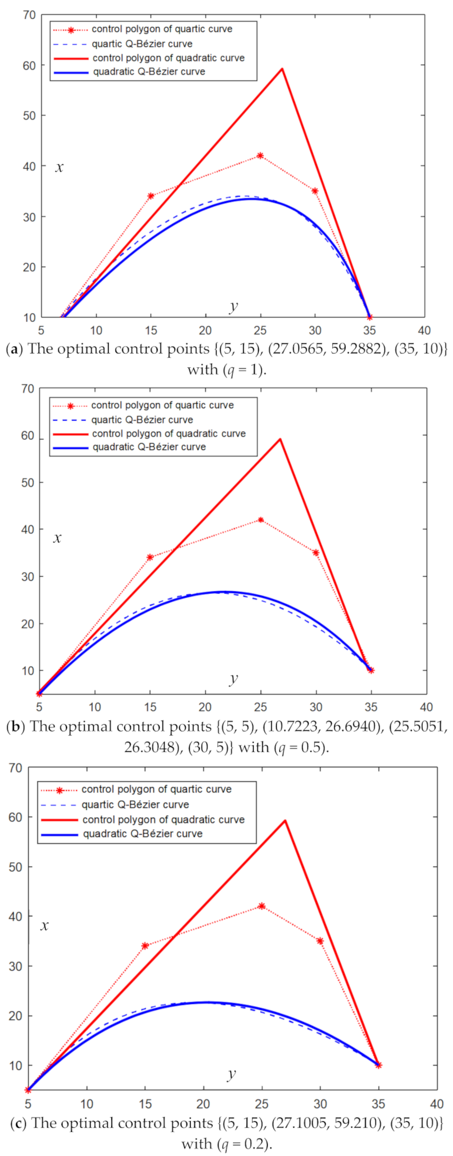
Figure 4 shows the two-degree reduction of a quartic Q-Bézier curve, whose control points are {T₀ = (5, 5), T₁ = (15, 34), T₂ = (25, 42), T₃ = (30, 35), T₄ = (35, 10)}. With q = 1, the original quartic Q-Bézier curve (blue dot line) and the approximating quadratic Q-Bézier curve (blue solid line) are shown in Figure 4a. Another two pairs of generated Q-Bézier curves with q = 0.5, q = 0.2 are, respectively, displayed in Figure 4b,c.

Example 4.

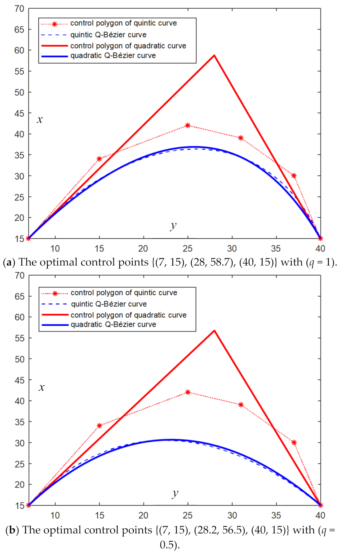
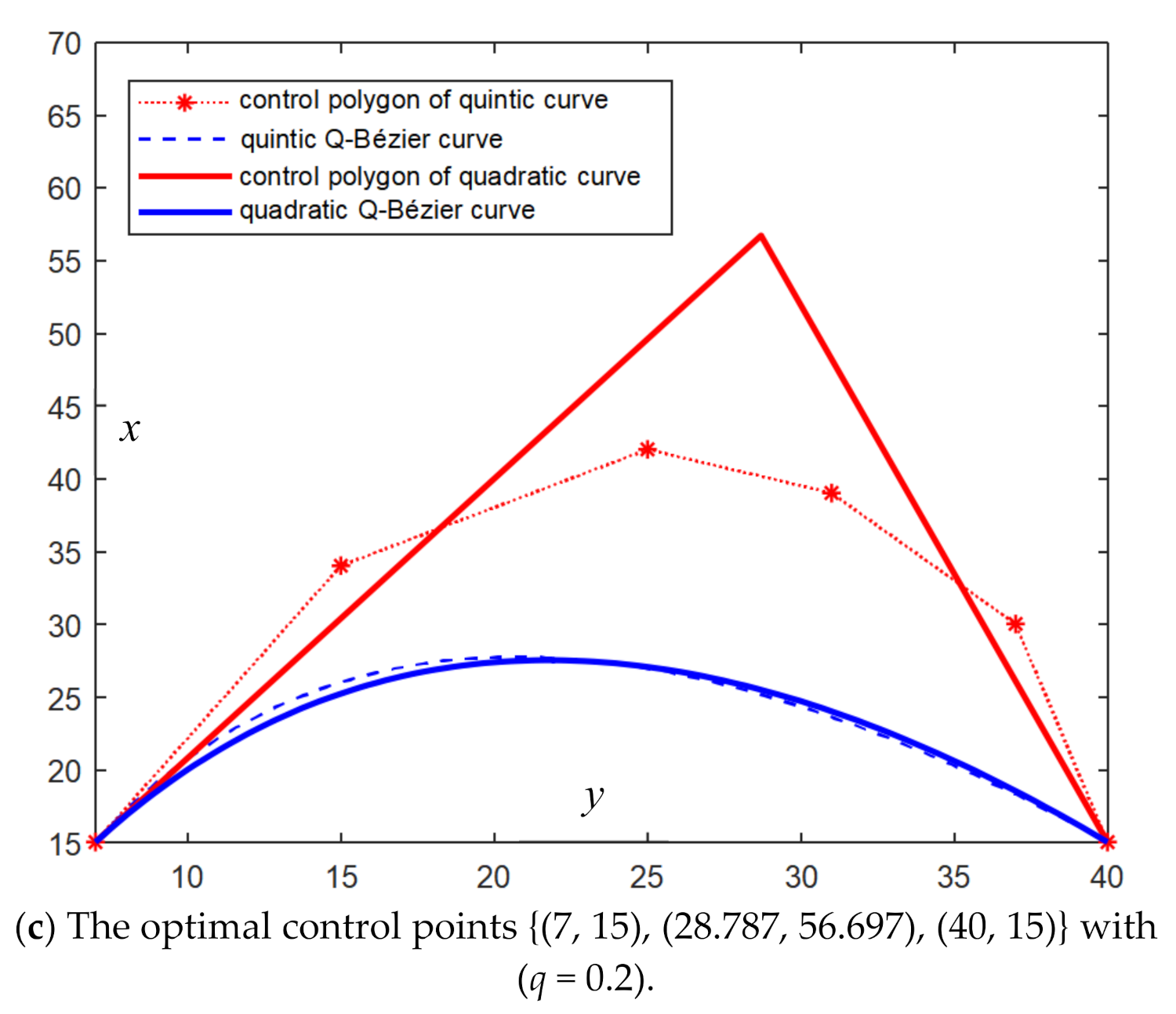
Figure 5 shows the three-degree reduction of a quintic Q-Bézier curve, whose control points are {T₀ = (7, 15), T₁ = (15, 34), T₂ = (25, 42), T₃ = (31, 39), T₄ = (37, 30), T₅ = (40, 15)}. With q = 1, the original quintic Q-Bézier curve (blue dot line) and the approximating quadratic Q-Bézier curve (blue solid line) are shown in Figure 5a. Another two pairs of generated Q-Bézier curves with q = 0.5, q = 0.2 are, respectively, displayed in Figure 5b,c. As can be seen from Figure 5, with the change of the shape parameter q, the effect of multiple-degree reduction of the Q-Bézier curves does not change significantly.

Example 5.

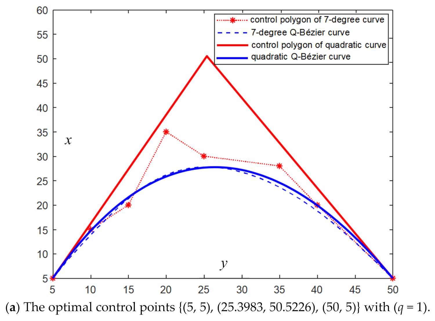
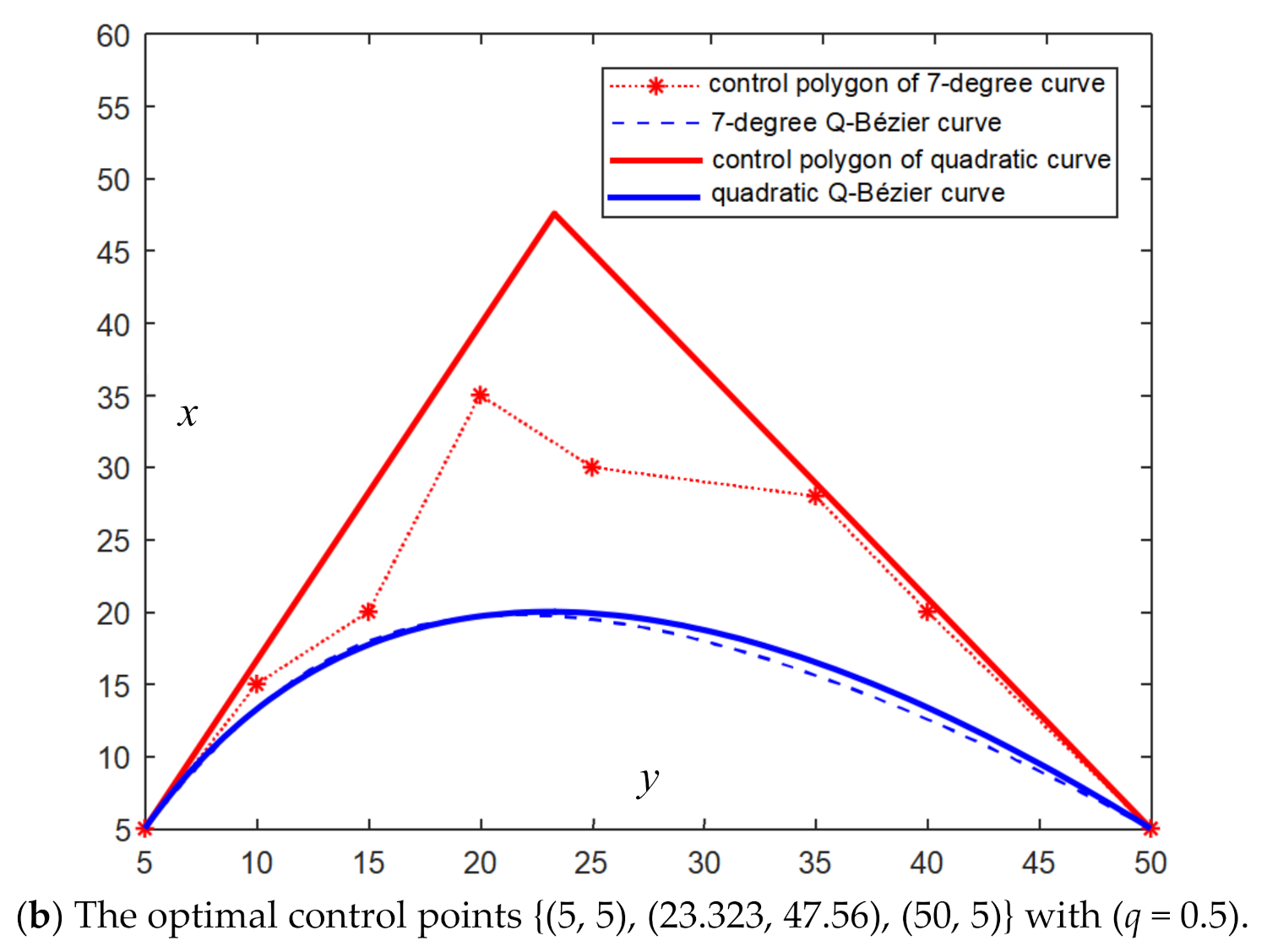
Figure 6 shows the five-degree reduction of a Q-Bézier curve of degree 7, whose control points are { T₀ = (5, 5), T₁ = (10, 15), T₂ = (15, 20), T₃ = (20, 35), T₄ = (25, 30), T₅ = (35, 28), T₆ = (40, 20), T₇ = (50, 5)}. With q = 1, the original Q-Bézier curve of degree 7 (blue dot line) and the approximating Q-Bézier curve of degree 2 (blue solid line) are shown in Figure 6a. Another pair of curves with q = 0.5 is displayed in Figure 6b. Analogously, the change of the shape parameter q will slightly affect the effect of the five-degree reduction of the Q-Bézier curves, which is consistent with the conclusion in Example 4. However, the shapes of the control polygon for the approximating curves change significantly with the change of the shape parameter q.

Example 6.

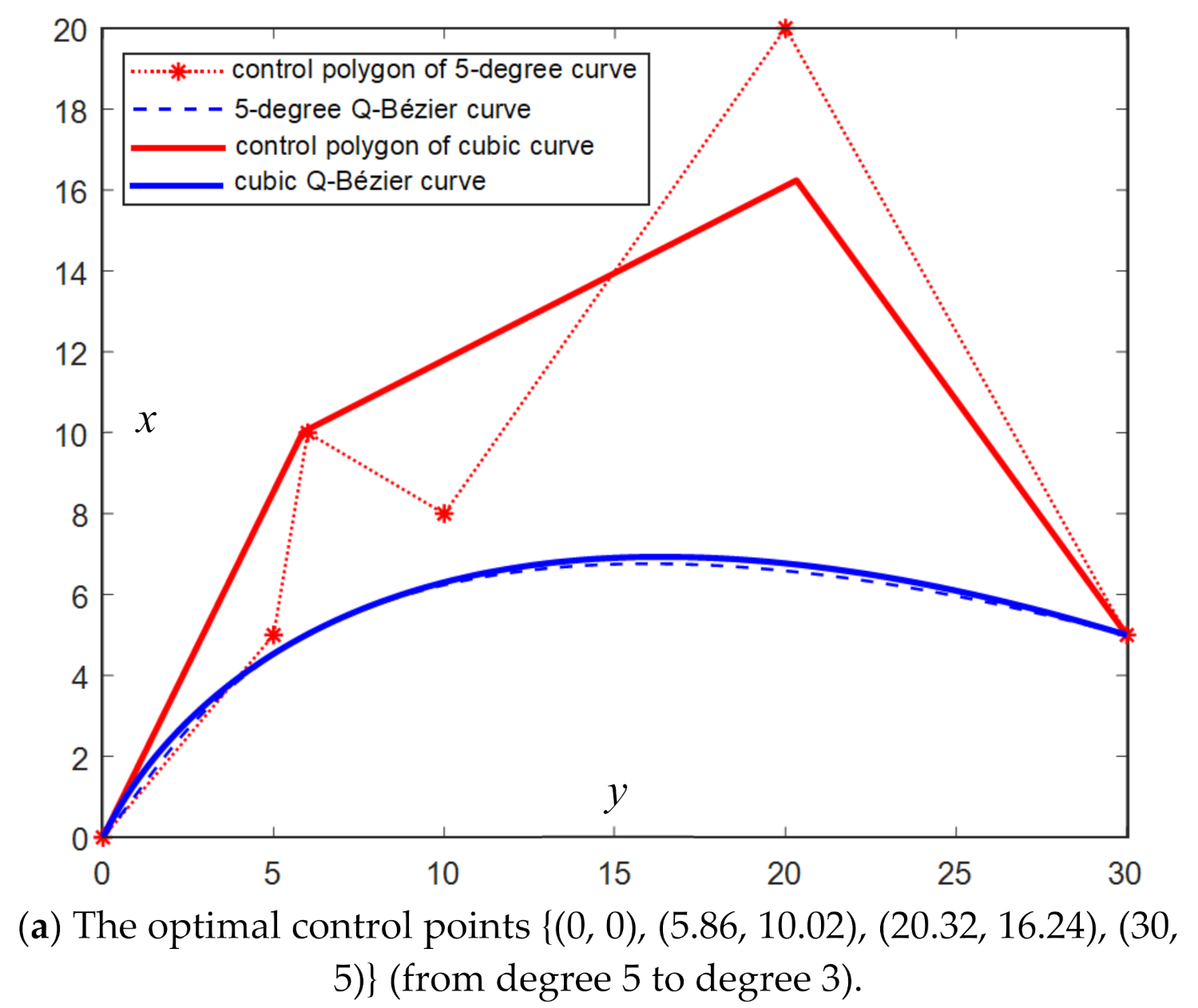
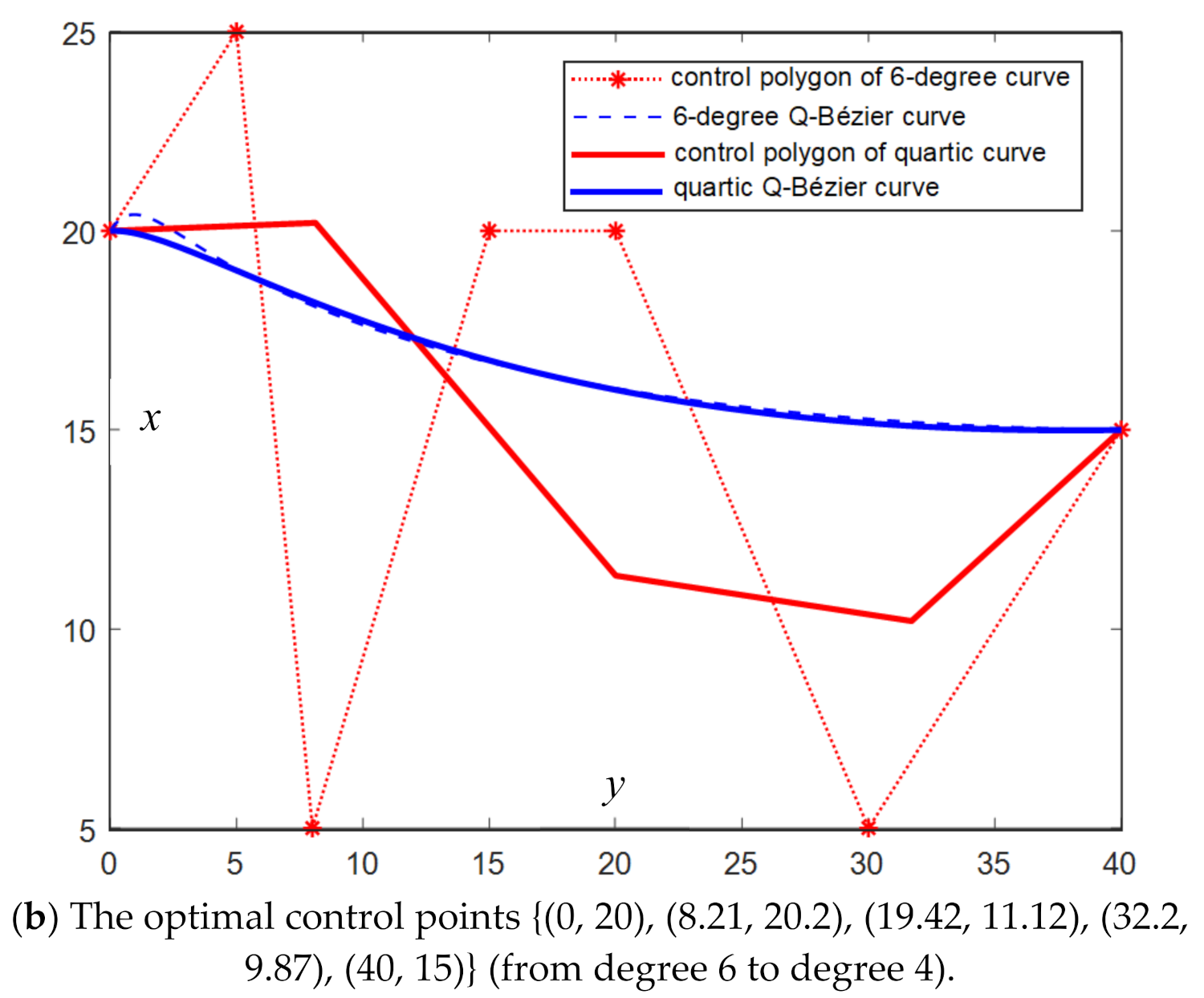
Figure 7 shows the two-degree reductions of two Q-Bézier curves of degree 5 and degree 6, whose control points are { T₀ = (0, 0), T₁ = (5, 5), T₂ = (6, 10), T₃ = (10, 8), T₄ = (20, 20), T₅ = (30, 5)} and { T₀ = (0, 20), T₁ = (5, 25), T₂ = (8, 5), T₃ = (15, 20), T₄ = (20, 20), T₅ = (30, 5), T₆ = (40, 15)}, respectively. With q = 0.2, the original Q-Bézier curve of degree 5 (blue dot line) and the approximating Q-Bézier curve of degree 3 (blue solid line) are shown in Figure 7a. Another example for Two-degree reduction of Q-Bézier curves of degree 6 is shown in Figure 7b. As seen from Figure 7, the effect of the two-degree reductions of fifth-degree and sixth-degree Q-Bézier curves are both very good. Furthermore, the changes of the shape parameter q have little effect on the degree reduction results of the curves.

5.3. Results Discussion

Obviously, as can be seen from Figure 2, Figure 3, Figure 4, Figure 5, Figure 6 and Figure 7, the degree reduced Q-Bézier curves exhibit good approximation effect to the original Q-Bézier curves, which demonstrates that the proposed algorithm works well for the multiple-degree reduction of Q-Bézier curves. This section shows the errors of degree reduction of six numerical examples to illustrate the accuracy and availability of the proposed methods.

As previously mentioned, the L₂-norm-based error function in (19) can be used to measure the approximation effect between the degree reduced Q-Bézier curves and the original Q-Bézier curves. Nevertheless, the error calculated by the function in Equation (19) is an absolute error, and its value is affected by the coordinate value of the control points of the curves, which brings inconvenience to the objective evaluation of the approximation effect. Therefore, in this paper, a new relative error function of degree reduction

$$\stackrel{\sim }{\epsilon }={\stackrel{\sim }{d}}_{L_2}(y(\eta ),z(\eta ))={\displaystyle \underset{0}{\overset{1}{\int }}\left|\right|y(\eta )-z(\eta )|{|}^2}d\eta /{\displaystyle \underset{0}{\overset{1}{\int }}\left|\right|y(\eta )|{|}^2}d\eta$$

(20)

is used for measuring the approximation effect between the degree reduced Q-Bézier curves and the original Q-Bézier curves. The relative errors of the degree reductions in Figure 2, Figure 3, Figure 4, Figure 5, Figure 6 and Figure 7 are shown in

Table 1. The errors of degree reduction for the examples in Figure 2, Figure 3, Figure 4, Figure 5, Figure 6 and Figure 7.

Figures	The Relative Error $\overline{\mathit{\epsilon }}$ of Each Subgraph in the Figures.
	Subgraph (a)	Subgraph (b)	Subgraph (c)
Figure 2	6.0424 × 10−3	6.8459 × 10−3	/
Figure 3	5.4410 × 10−2	2.4315 × 10−3	/
Figure 4	1.3256 × 10−2	6.2817 × 10−2	9.9295 × 10−3
Figure 5	1.0293 × 10−3	1.3858 × 10−2	2.6748 × 10−2
Figure 6	4.6859 × 10−3	1.3298 × 10−2	/
Figure 7	8.5823 × 10−3	3.2906 × 10−3	/

Note: “/” indicates that there is no corresponding subgraph in the Figure 2 and Figure 3 and Figure 6 and Figure 7.

.

As for the influence of the maximum iterations M on the approximation effect, it is obvious that with the increase of the number of iterations, the error value $\overline{\epsilon }$ decreases gradually in the initial iterations; when the iterative number reaches a certain threshold, the error value $\overline{\epsilon }$ will keep unchanged despite the increased number of iterations. In our experiments, when the maximum iteration M reaches 40~60, there is usually no dramatic decrease in the error value $\overline{\epsilon }$. Since high-maximum iterations will significantly reduce the computational efficiency, we set the maximum iteration M in our experiments as 50.

5.4. Comparison of SSA with other SIA-Based Methods

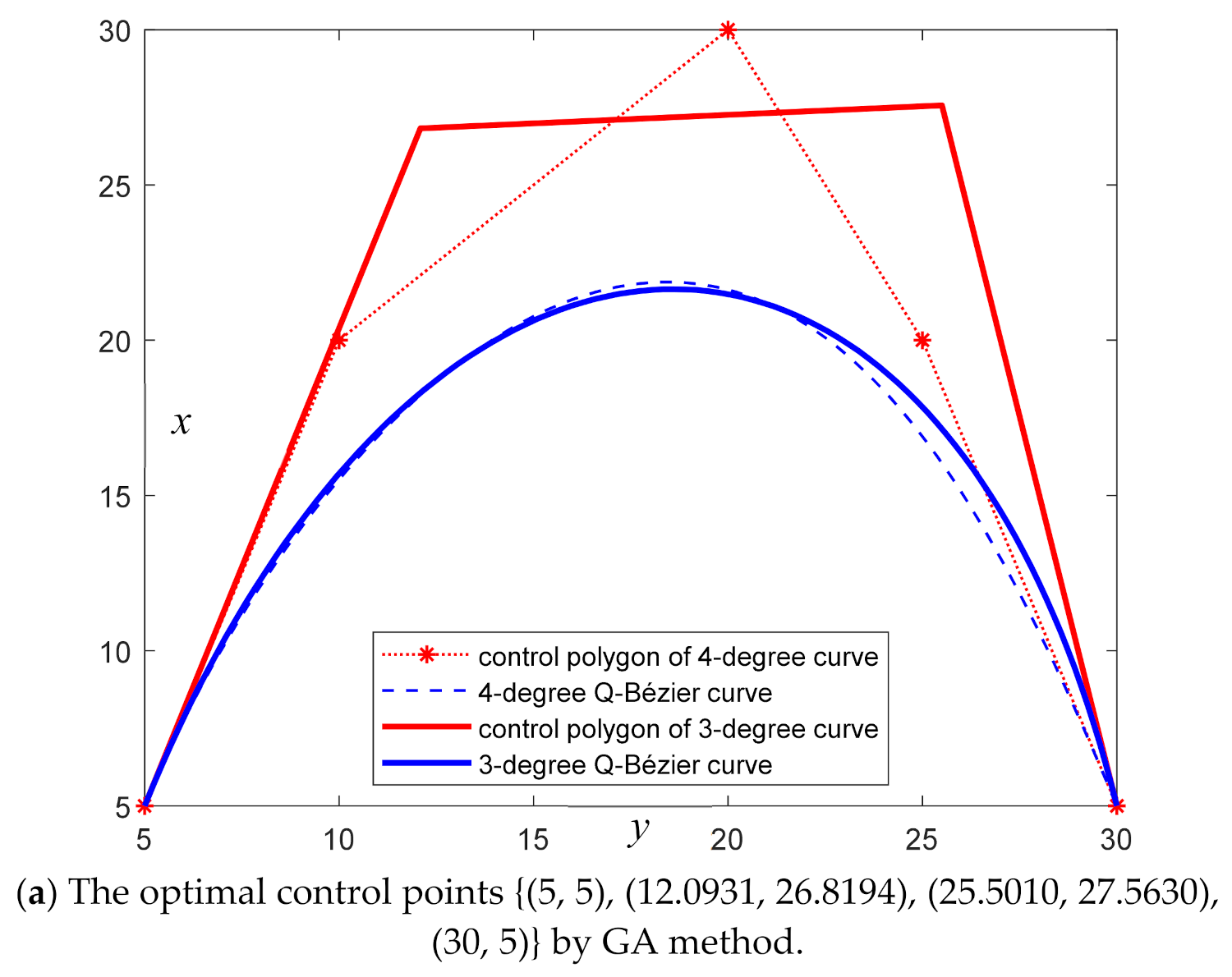
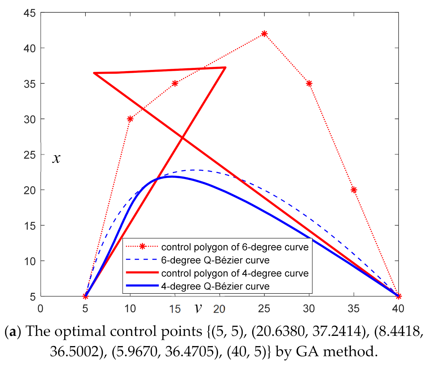
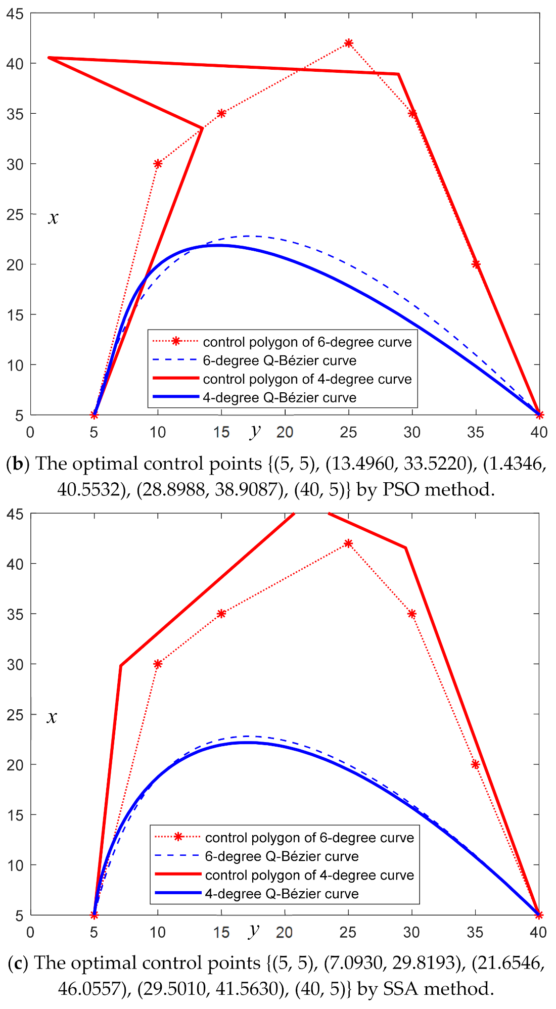
Scholars have carried out a lot of research on the degree reduction of classical Bézier curves, see [22,23,24,25,26,27,28,29,30]. Regrettably, these degree reduction methods in [22,23,24,25,26,27,28,29,30] cannot be directly extended to solve the degree reduction problem of Q-Bézier curves. On this account, we studied the degree reduction of Q-Bézier curves using the squirrel search algorithm in this paper. In order to verify the performance of the proposed method, in this section, we gave some comparisons of the SSA method (i.e., our method) with the genetic algorithm (GA) method and the PSO method. Here, the GA method and PSO method refer to degree reduction of Q-Bézier curves using the GA and PSO, respectively. That is, the GA and PSO are used to solve the degree reduction model of Q-Bézier curves in (15). Figure 8 and Figure 9 show the comparisons of degree reduction effects among the GA method, the PSO method and the SSA method under the shape parameter q = 1 and q = 0.2, respectively. In Figure 8, the curve before degree reduction is a fourth of the Q-Bézier curve whose control points are {T₀ = (5, 5), T₁ = (10, 20), T₂ = (20, 30), T₃ = (25, 20), T₄ = (30, 5)} and shape parameter q is 1; the curve after degree reduction is a third of the Q-Bézier curve. In Figure 9, the curve before degree reduction is a sixth of the Q-Bézier curve whose control points are {T₀ = (5, 5), T₁ = (10, 30), T₂ = (15, 35), T₃ = (25, 42), T₄ = (30, 35), T₅ = (35, 20), T₆ = (40, 5)} and shape parameter q is 0.2; the curve after degree reduction is a fourth of the Q-Bézier curve.

Table 2. The errors of degree reduction for the comparison in Figure 8 and Figure 9.

Figures	The Relative Error $\overline{\mathit{\epsilon }}$ of Each Subgraph in the Figures
	Subgraph (a)	Subgraph (b)	Subgraph (c)
Figure 8	1.7832 × 10−4	7.4585 × 10−4	1.3352 × 10−4
Figure 9	5.1891 × 10−3	3.0882 × 10−3	2.3990 × 10−3

shows the error comparisons of the three degree reduction methods in Figure 8 and Figure 9. Apparently, from Figure 8 and Figure 9 and Table 2, the SAA method is better than the GA method and PSO method, which apparently indicates the performance of our method.

6. Conclusions

This paper proposes a new method for the multiple-degree reduction of Q-Bézier curves by incorporating the squirrel search algorithm (SSA). By our method, the optimal sequence of control points for the degree reduced Q-Bézier curve can be found intelligently. The examples show the superiorities and potential possessed by squirrel search algorithm in multiple-degree reduction of Q-Bézier curve. Therefore, this method is applicable for CAD/CAM modeling systems. A promising and important direction for future work is to incorporate more high-efficient nature-inspired algorithms for the shape optimization of curves and surfaces, in which shape parameters can also be taken as the decision variables.

References

- Bieri, H.P.; Prautsch, H. Preface. Comput. Aided Geom. Des. 1999, 16, 579–581. [Google Scholar] [CrossRef]
- Farin, G. Curves and Surfaces for CAGD: A Practical Guide, 5th ed.; Academic Press: San Diego, CA, USA, 2002; pp. 227–238. [Google Scholar]
- Mamar, E. Shape preserving alternatives to the rational Bézier model. Comput. Aided Geom. Des. 2001, 18, 37–60. [Google Scholar] [CrossRef]
- Hu, G.; Wu, J.; Qin, X. A novel extension of the Bézier model and its applications to surface modeling. Adv. Eng. Softw. 2018, 125, 27–54. [Google Scholar] [CrossRef]
- Hu, G.; Bo, C.; Wu, J.; Wei, G.; Hou, F. Modeling of Free-Form Complex Curves Using SG-Bézier Curves with Constraints of Geometric Continuities. Symmetry 2018, 10, 545. [Google Scholar] [CrossRef] [Green Version]
- Hu, G.; Bo, C.C.; Wei, G.; Qin, X.Q. Shape-adjustable generalized Bézier Surfaces: Construction and its geometric continuity conditions. Appl. Math. Comput. 2020, 378, 125215. [Google Scholar] [CrossRef]
- Hu, G.; Wu, J.; Qin, X. A new approach in designing of local controlled developable H-Bézier surfaces. Adv. Eng. Softw. 2018, 121, 26–38. [Google Scholar] [CrossRef]
- Hu, G.; Wu, J. Generalized quartic H-Bézier curves: Construction and application to developable surfaces. Adv. Eng. Softw. 2019, 138, 15. [Google Scholar] [CrossRef]
- BiBi, S.; Abbas, M.; Misro, M.Y.; Hu, G. A novel approach of hybrid trigonometric Bézier curve to the modeling of symmetric revolutionary curves and symmetric rotation surfaces. IEEE Access 2019, 7, 165779–165792. [Google Scholar] [CrossRef]
- BiBi, S.; Abbas, M.; Miura, K.T.; Misro, M.Y. Geometric modeling of novel Generalized hybrid Trigonometric Bézier-like curve with shape Parameters and its applications. Mathematics 2020, 8, 967. [Google Scholar] [CrossRef]
- Phillips, G.M. Bernstein polynomials based on the q-integers. Ann. Numer. Math. 1997, 4, 511–518. [Google Scholar]
- Oruc, H.; Phillips, G.M. q-Bernstein polynomials and Bézier curves. J. Comput. Appl. Math. 2003, 151, 1–12. [Google Scholar] [CrossRef] [Green Version]
- Disibuyuk, C.; Oruc, H. A generalization of rational Bernstein-Bézier curves. BIT Numer. Math. 2007, 47, 313–323. [Google Scholar] [CrossRef]
- Simeonov, P.; Zafiris, V.; Goldman, R. q-Blossoming: A new approach to algorithms and identities for q-Bernstein bases and q-Bézier curves. J. Approx. Theory 2012, 164, 77–104. [Google Scholar] [CrossRef] [Green Version]
- Goldman, R.; Simeonov, P.; Simsek, Y. Generating Functions for the q-Bernstein Bases. SIAM J. Discrete Math. 2014, 28, 1009–1025. [Google Scholar] [CrossRef]
- Han, L.W.; Chu, Y.; Qiu, Z.Y. Generalized Bézier curves and surfaces based on Lupaş q-analogue of Bernstein operator. J. Comput. Appl. Math. 2014, 261, 352–363. [Google Scholar] [CrossRef]
- Han, L.-W.; Wu, Y.-S.; Chu, Y. Weighted Lupaş q-Bézier curves. J. Comput. Appl. Math. 2016, 308, 318–329. [Google Scholar] [CrossRef]
- Lu, L.; Jiang, C.; Xiang, X. Some remarks on weighted Lupaş q-Bézier curves. J. Comput. Appl. Math. 2017, 313, 393–396. [Google Scholar] [CrossRef]
- Hu, G.; Bo, C.; Qin, X. Continuity conditions for tensor product Q-Bézier surfaces of degree (m,n). Comp. Appl. Math. 2018, 37, 4237–4258. [Google Scholar] [CrossRef]
- Jegdić, I.; Simeonov, P.; Zafiris, V. Quantum (q, h)-Bézier surfaces based on bivariate (q, h)-blossoming. Demonstr. Math. 2019, 52, 451–466. [Google Scholar]
- Delgado, J.; Peña, J.M. Geometric properties and algorithms for rational q-Bézier curves and surfaces. Mathematics 2020, 8, 541. [Google Scholar] [CrossRef] [Green Version]
- Zhao, Y. Research on degree reduction of C-Bézier curves Based on generalized inverse matrix. Netw. Secur. Technol. Appl. 2010, 12, 38–40. [Google Scholar]
- Chen, G.; Wang, G.J. Degree reduction approximation of Bézier curves by generalized inverse matrices. J. Comput. Aided Des. Comput. Graph. 2001, 12, 435–439. [Google Scholar]
- Cai, H.; Wang, G. Constrained approximation of rational Bézier curves based on a matrix expression of its end points continuity condition. Comput.-Aided Des. 2010, 42, 495–504. [Google Scholar] [CrossRef]
- Gospodarczyk, P. Degree reduction of Bézier curves with restricted control points area. Comput.-Aided Des. 2015, 62, 143–151. [Google Scholar] [CrossRef]
- Ahn, Y. Using Jacobi polynomials for degree reduction of Bézier curves with Ck-constraints. Comput. Aided Geom. Des. 2003, 20, 423–434. [Google Scholar] [CrossRef]
- Lee, B.; Park, Y.; Yoo, J. Application of Legendre-Bernstein basis transformations to degree elevation and degree reduction. Comput. Aided Geom. Des. 2002, 19, 709–718. [Google Scholar] [CrossRef] [Green Version]
- Rababah, A.; Lee, B.; Yoo, J. A simple matrix form for degree reduction of Bézier curves using Chebyshev-Bernstein basis transformations. Appl. Math. Comput. 2006, 181, 310–318. [Google Scholar] [CrossRef]
- Ahn, Y.J.; Lee, B.G.; Park, Y.; Yoo, J. Constrained polynomial degree reduction in the L2-norm equals best weighted Euclidean approximation of Bézier coefficients. Comput. Aided Geom. Des. 2004, 21, 181–191. [Google Scholar] [CrossRef]
- Ait-Haddou, R.; Bartoň, M. Constrained multi-degree reduction with respect to Jacobi norms. Comput. Aided Geom. Des. 2016, 42, 23–30. [Google Scholar] [CrossRef] [Green Version]
- Lu, J.; Qin, X. Degree reduction of S-λ curves using a genetic simulated annealing algorithm. Symmetry 2019, 11, 15. [Google Scholar] [CrossRef] [Green Version]
- Hu, G.; Qiao, Y.; Qin, X.Q.; Guo, W. Approximate multi-degree reduction of SG-Bézier curves using the grey wolf optimizer algorithm. Symmetry 2019, 11, 1242. [Google Scholar] [CrossRef] [Green Version]
- Qin, X.; Qiao, Y.; Hu, G. Degree reduction of SG-Bézier surfaces based on grey wolf optimizer. Math. Meth. Appl. Sci. 2020, 43, 6416–6429. [Google Scholar] [CrossRef]
- Guo, W.Y.; Liu, T.; Dai, F.; Zhao, F.; Xu, P. Skewed normal cloud modified whale optimization algorithm for degree reduction of S-λ curves. Appl. Intell. 2021, 1–22. [Google Scholar] [CrossRef]
- Hu, G.; Zhu, X.N.; Wei, G.; Chang, C.T. An improved marine predators algorithm for shape optimization of developable Ball surfaces. Eng. Appl. Artif. Intell. 2021, 105, 104417. [Google Scholar] [CrossRef]
- Kennedy, J.; Eberhart, R.C. Particle swarm optimization. In Proceedings of the IEEE International Conference on Neural Networks, Perth, Australia, 27 November–1 December 1995; pp. 1942–1948. [Google Scholar]
- Mirjalili, S.; Mirjalili, S.M.; Lewis, A. Grey wolf optimizer. Adv. Eng. Softw. 2014, 69, 46–61. [Google Scholar] [CrossRef] [Green Version]
- Mirjalili, S.; Lewis, A. The Whale Optimization Algorithm. Adv. Eng. Softw. 2016, 95, 51–67. [Google Scholar] [CrossRef]
- Mirjalili, S.; Gandomi, A.H.; Mirjalili, S.Z.; Saremi, S.; Faris, H.; Mirjalili, S.M. Salp swarm algorithm: A bio-inspired optimizer for engineering design problems. Adv. Eng. Soft. 2017, 114, 163–191. [Google Scholar] [CrossRef]
- Saremi, S.; Mirjalili, S.; Lewis, A. Grasshopper Optimisation Algorithm: Theory and application. Adv. Eng. Softw. 2017, 105, 30–47. [Google Scholar] [CrossRef] [Green Version]
- Heidari, A.A.; Mirjalili, S.; Faris, H.; Aljarah, I.; Mafarja, M.; Chen, H. Harris hawks optimization: Algorithm and applications. Futur. Gener. Comput. Syst. 2019, 97, 849–872. [Google Scholar] [CrossRef]
- Jain, M.; Singh, V.; Rani, A. A novel nature-inspired algorithm for optimization: Squirrel search algorithm. Swarm Evol. Comput. 2019, 44, 148–175. [Google Scholar] [CrossRef]
- Lavanya, N.; Shankar, T. Energy efficient cluster head selection using squirrel search algorithm in wireless sensor networks. J. Commun. 2020, 15, 528–536. [Google Scholar] [CrossRef]
- Deb, D.; Roy, S. Brain tumor detection based on hybrid deep neural network in MRI by adaptive squirrel search optimization. Ultimed. Tools Appl. 2020, 80, 2621–2645. [Google Scholar] [CrossRef]
- Yang, X. Firefly Algorithm, Lévy Flights and Global Optimization; Springer: London, UK, 2010; pp. 209–218. [Google Scholar]
- Rababah, A.; Mann, S. Iterative process for G2-multi degree reduction of Bézier curves. Appl. Math. Comput. 2011, 217, 8126–8133. [Google Scholar] [CrossRef]
Figure 1.
The cubic Q-Bézier curve with the shape parameter q increasing (from bottom to the top).
Figure 2.
One-degree reduction of a cubic Q-Bézier curve with the shape parameter q = 1, 0.5.
Figure 3.
One-degree reduction of a quartic Q-Bézier curve with the shape parameter q = 1, 0.5.
Figure 4.
Two-degree reduction of a quartic Q-Bézier curve with the shape parameter q = 1, 0.5, 0.2.
Figure 5.
Three-degree reduction of a quartic Q-Bézier curve with the shape parameter q = 1, 0.5, 0.2.
Figure 6.
Five-degree reductions of a Q-Bézier curve of degree 7 with the shape parameter q = 1, 0.5.
Figure 7.
Two-degree reductions of a Q-Bézier curve of degree 5 and degree 6.
Figure 8.
Comparisons of one-degree reduction among GA method, PSO method and SSA method; under C0 constraint condition.
Figure 9.
Comparisons of two-degree reduction among GA method, PSO method, and SSA method; under C0 constraint condition.