
Genetic Hybrid Optimization of a Real Bike Sharing System
by
 , , and
Gonzalo A. Aranda-Corral
1,† ,
,
Miguel A. Rodríguez
1,†,
Iñaki Fernández de Viana
1,† and
María Isabel G. Arenas
2,*,† 1
Department Information Technologies, University of Huelva, 21007 Huelva, Spain
2
Department Computer Architecture and Computer Technology, ETSIIT-CITIC, University of Granada, 18071 Granada, Spain
*
Author to whom correspondence should be addressed.
†
These authors contributed equally to this work.
Mathematics 2021, 9(18), 2227; https://0-doi-org.brum.beds.ac.uk/10.3390/math9182227
Submission received: 31 July 2021
/
Revised: 3 September 2021
/
Accepted: 5 September 2021
/
Published: 10 September 2021
(This article belongs to the Special Issue Applications of Evolutionary Algorithms)
Abstract
:In recent years there has been a growing interest in resource sharing systems as one of the possible ways to support sustainability. The use of resource pools, where people can drop a resource to be used by others in a local context, is highly dependent on the distribution of those resources on a map or graph. The optimization of these systems is an NP-Hard problem given its combinatorial nature and the inherent computational load required to simulate the use of a system. Furthermore, it is difficult to determine system overhead or unused resources without building the real system and test it in real conditions. Nevertheless, algorithms based on a candidate solution allow measuring hypothetical situations without the inconvenience of a physical implementation. In particular, this work focuses on obtaining the past usage of bike loan network infrastructures to optimize the station’s capacity distribution. Bike sharing systems are a good model for resource sharing systems since they contain common characteristics, such as capacity, distance, and temporary restrictions, which are present in most geographically distributed resources systems. To achieve this target, we propose a new approach based on evolutionary algorithms whose evaluation function will consider the cost of non-used bike places as well as the additional kilometers users would have to travel in the new distribution. To estimate its value, we will consider the geographical proximity and the trend in the areas to infer the behavior of users. This approach, which improves user satisfaction considering the past usage of the former infrastructure, as far as we know, has not been applied to this type of problem and can be generalized to other resource sharing problems with usage data.
1. Introduction
Bikes usage in cities has seen a dramatic increase in popularity, both in big and medium size cities, with more than 2000 cities with a bike share program [1] and more than 3.5 million bikes [2]. Some of the main concerns in big cities are contamination and traffic jams; in 2016, bike sharing in Shanghai saved 8358 tonnes of petrol and decreased CO2 and NOX emissions by 25,240 and 64 tonnes, respectively [3]. Both, governments and citizens are pushing a new paradigm of mobility based on bike transportation. Nevertheless, crowded cities lack space for parking in central areas, and as reported by [4], dock-less bikes exist in limbo between disposable and valuable, which makes them a target for abuse and abandonment. To bring some ease, using such appropriate opportunities and circumstances, a new model of bike sharing has been [5] taking place in the last few years: Bike Sharing Systems (BSS). Based on the principle of a vehicle as a service, a new wave of city institutions has implemented networks of docks in a park with shared bikes. This strategy boosts the fluidity of traffic and keeps [6] the public space under control, preventing the users from using their own bikes.
The numbers speak for themselves, as one shared bike can be used several times by different users with all the added benefits of bike transportation [7]: lower noise, and improvement of physical and mental well-being for users and citizens, etc.
The operation of this network implies several problems, but we could consider that the key of the system is user satisfaction. In [8], a study is conducted in the context of bicycle sharing that identifies the aspects considered as most important for the customers. A priori, it may appear that the biggest challenges to developing bike sharing systems for sustainability are related to geographical considerations: rain, snow, high or freezing temperatures, and other adverse weather conditions [9]; but one of the most common complaints in vehicle sharing networks is availability: when users cannot find a bike nearby or cannot find a dock to leave the bike, the sustainability of the system is in danger. The system is unbalanced by nature, mainly caused by the asymmetry of demand between variable requests and returns at different zones. i.e., the usage of Bicycle Sharing Systems (BSS) brings the casuistry of traffic to the parking docks, i.e., peak hours and unbalanced usage. Downtowns, universities and commercial areas act as sinks of bikes while residential areas supply them. Ideally, at the end of the day the bikes will return to fill the original places when users may occasionally return to their original departure. Several dynamic protocols are in place to keep the number of bikes and places low: dynamic bike redistribution, in which a truck redistributes, during the day, bikes from sinks to sources with price incentives to ensure the system balanced is balanced [10]. The right number of places and bikes that the network has to have in any of these situations is a study case not yet solved. We can rely on a daily redistribution, real-time redistribution or even on an oversized fleet and docking network, but having the correct dimensions of fleet and docks in comparison with the needs is a must [11] to keep the system sustainable.
1.1. Capacity Distribution Problem
The other aspect to consider is the fixed part of the network: docks; these elements are urban furniture with elevated costs of planning, execution and maintenance [12]. Even an oversized network may not be optimal because of the inner distribution of docking places in the city. Due to the nature of urban infrastructures, most of the effort on network capacity is focused on design and implementation, based on general assumptions over user interests in city zones.
The uncertainty over the behavior of such a complex system will be cleared up once the system is alive. The network reliability is usually measured with the percentage of times the network of bikes/docks are unusable because those dead periods will ultimately derive from lost requests, either by a user that cannot find a place to hold the bike or by not having a bike in a station for being picked up.
There are many proposals that optimize network distribution capacity. The authors of [13] consider the number of bikes, and the authors of [14] consider the dynamic reallocation of bikes. The allocation of the layout is handled in [15], which relies on the idea of cluster and a greedy heuristic.
There have been a number of studies examining BSS functionality and human biking behavior. The authors of [16] cited two types of data used in BSS bike sharing research: based on automatics stocks (stations) and on trips. This paper states that stock-based analysis hardly reflects movement patterns across a city, but it reflects fluctuation in demand and availability. Stock-based data have analyzed prediction over availability: in [17], the authors studied the stock behavior through clustering to give an availability prediction in Barcelona BSS, and in [18], they had a similar outcome in Paris.
1.2. Capacity and User Satisfaction Optimization over a Real Usage Simulation
Reference [19] uses an optimization that considers network reliability by means of two concepts, zero-vehicle time and full-port time, which reflected the duration of vehicle shortage and parking stall unavailability in the stations, respectively. Nevertheless, this proposal introduces lost users of the system, bringing the concept of user satisfaction, i.e., not forcing the user to travel to other stations or turn/shift to other travel modes. The most accepted measures in the literature are the ones based on the unsatisfied demands of users.
Other authors measure the same concept of loss of opportunity with different naming but the same indirect calculations based on empty/saturated stations and a probability of requests over time. References [20,21] identify problematic stations where users are unable to obtain a bike or a place over time.
The capacity distribution over existing stations, considering user satisfaction and budget as the number of docks needed at each station, is a combinatorial problem with an exponential number of possible solutions.
The concept of user satisfaction in [22] measures the probability of a request being held over a period of time by means of a randomized simulation on request. Even being based on usage, from our point of view, this approach lacks granularity. In big cities, it is common to have several stations in the same place or very close to each other, and the user may use one of them after not finding an available place nearby.
This work proposes the combination of two metrics of the BSS performance:
- User satisfaction, based on the number of kilometers that a user has to walk or ride in order to pick up a bike or leave the bike in a closer station when the one that was originally selected is respectively empty or full.
- Total spare capacity, defined as the percentage of empty docks relative to the number of total bicycles in the network to optimize the costs of the network without impacting functionality.
The main goal of this work is to maximize user satisfaction, taking into account the cost of the system and the limitations, in order to find the best distribution of the station capacities based on real usage.
2. Materials and Methods
This paper shows an optimization methodology based on candidate solution algorithms, such as local searches and genetic algorithms. In optimization, a candidate solution is a member of a set of possible solutions to a given problem. A candidate solution does not have to be a likely or reasonable solution to the problem—it is simply in the set that satisfies all constraints. Within this section, we will describe the problem, the candidate solution definition, the origin of our data, and the details of the algorithms that realize the optimization of the BSS capacity distribution.
2.1. The Origin of Data
The data used in this paper are distributed under the Open Licence from Etalab and were collected using the connector provided by JCDecaux [23]. This connector’s API provides, for a certain city, an extensive set of attributes in real-time. We have selected and retrieved the number of stations, capacity and occupation every 5 min, in order to figure out the dynamic of users. Within this interval, we will transform the occupation into requests of bikes or docks by means of subtracting consecutive occupation values.
The dataset is composed of the following fields: City as the name of the city, Station as a unique numeric identifier for the station in the city network, Capacity as the number of docks at the station, Docks and Bikes as the number of docks and bikes, respectively, that are available at the station. Latitude and Longitude for geographical location of the station and, finally, Date, as the instant of time where the measure was performed.
Table 1 shows a real sample of several tuples extracted over Santander city in April 2019. As named previously, these data are processed to produce the requests and also to calculate several non-time-dependent constants, such as distance between stations, number of bikes in the network, capacity of each station and total capacity.
2.2. Defining of a Candidate BSS
The candidate solution definition for the problem of capacity optimization of a BSS in a time frame can be defined as a city () that has a series of stations (S), each with an exact and constant capacity for the selected period that we are going to define. For this, we can use for the capacity vector of the city, with being the capacity of station j in this configuration.
We must denote that the study time will be for periods, so we will run the simulation over a windows time with discrete increments for 0 to . The capacity vector of a distribution will be constant over time.
The occupation matrix () keeps the occupation number of each station at every stage of the considered time window.
Note that is restricted to each station j in every moment to , that is, a station will not accept more bikes than the number of available docks. The remaining requests of docks will have to be redirected to other stations. Based on the premise that the number of available docks in the BSS has to be greater or equal to zero, we define spare capacity, , as the number of available docks when all the bikes are inside the stations in time j, and must always be positive (or zero).
The occupation matrix does not show the system’s dynamics needed to perform a simulation, just the status of each station at each time inside the time window; for this purpose, we are interested in capturing movements of bicycles, that is, the number of bicycles that are deposited or picked at a station between 2 consecutive instants of time.
In order to measure these movements, we used real data extracted from the source, as explained in Section 2.1.
We define and as the capacity and occupation captured from real data that will be transformed into dock/bike requests made over this time window. We call this the request matrix ():
In order to apply this over an alternative candidate solution, we assume that the initial state of the stations is empty. Therefore, the first request for every station will be the occupation at this time of the base case. Therefore, .
From now on, will reflect the behavior inherent to the real data recorder in the form of requests applied over a new capacity distribution (candidate solution). Consequently, this chain of requests may generate a different occupation sequence and lead to a redistribution of requests to other stations due to empty/full stations in the different capacity distribution.
2.3. Measuring the Performance of a Candidate BSS
The simulation of movements over a specific BSS capacity distribution reproduces the system state at a given time. From our knowledge, existing simulations on BSS uses mostly hourly demands averaged on weekdays that may not reflect particularities of some events due to the data averaging. Using real trends in an accumulative model may help gain a better understanding of the model limits without having to prove in detail the accuracy of the probabilities in generic simulations versus real conditions.
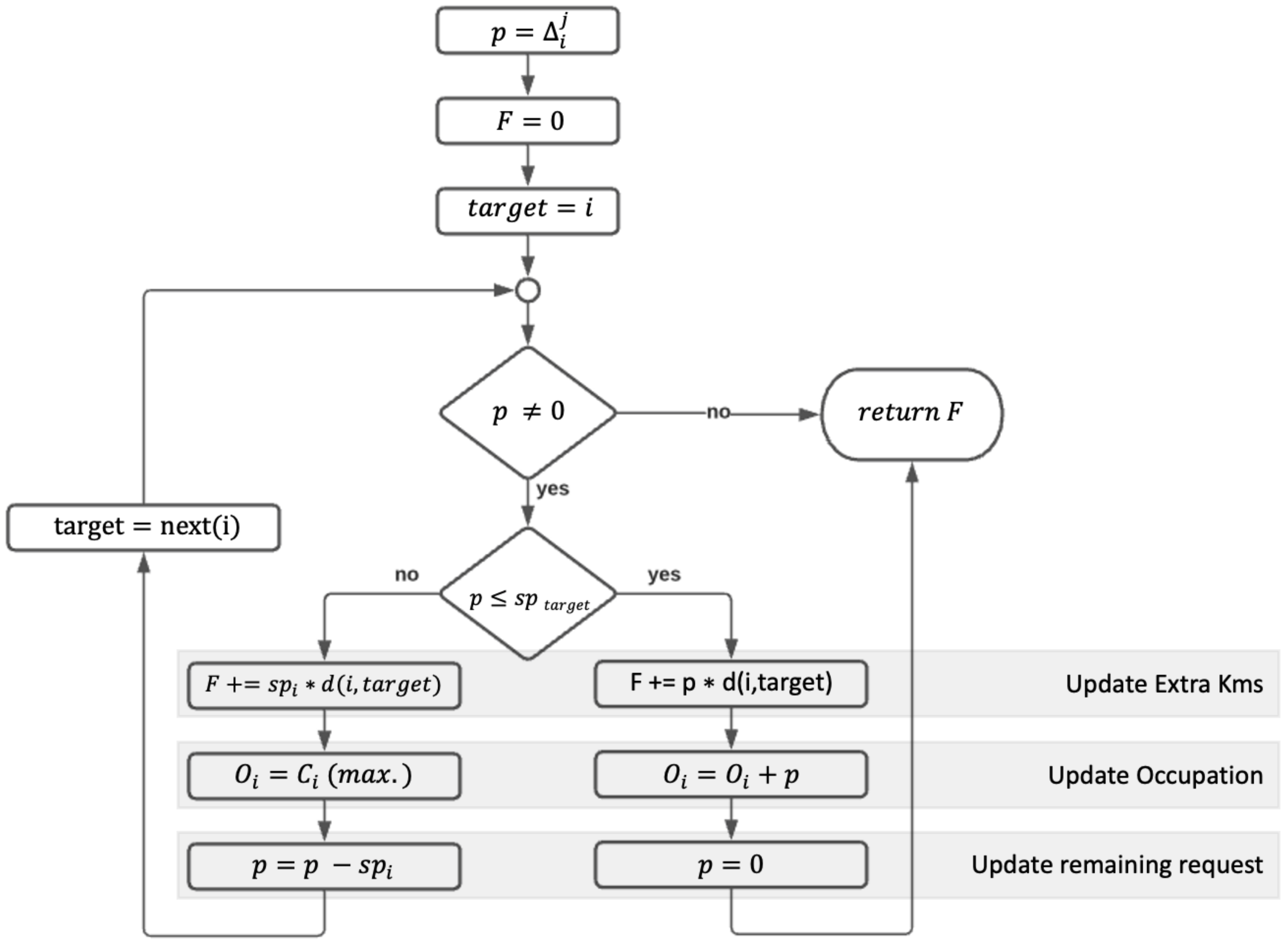
From the point of view of our simulation, each is interpreted as a request made by a user in a certain time j to obtain or to park a bike in a specific station i. The global process can be summarized as the distribution of requests (dock’s or bike’s demands) over a set of stations during a time interval from . Figure 1 presents the algorithm for request distribution in a candidate solution in which each station i in a time j will receive requests with an outcome measured in a number of kilometers performed by users when they have to travel from the original station to this new one due to a lack of places/bikes.
In the case that some requests (p) (either a bike or a dock) could not be attended by the current , we allocate as many as possible, updating the current occupation and p with the remaining .
The remaining requests (updated p) will be distributed, following the same process, in a set of distance ordered stations, from nearest to farthest, updating . Every time a request is attended by a station different from the original one where this request was recorded, the distance from this target to the original one will be added to a kilometer accumulator. This variable will keep the sum of kilometers traveled by the users due to failed requests (F) in the new distribution. The formula that measures the number of kilometers produced by the whole set of requests in the time window is:
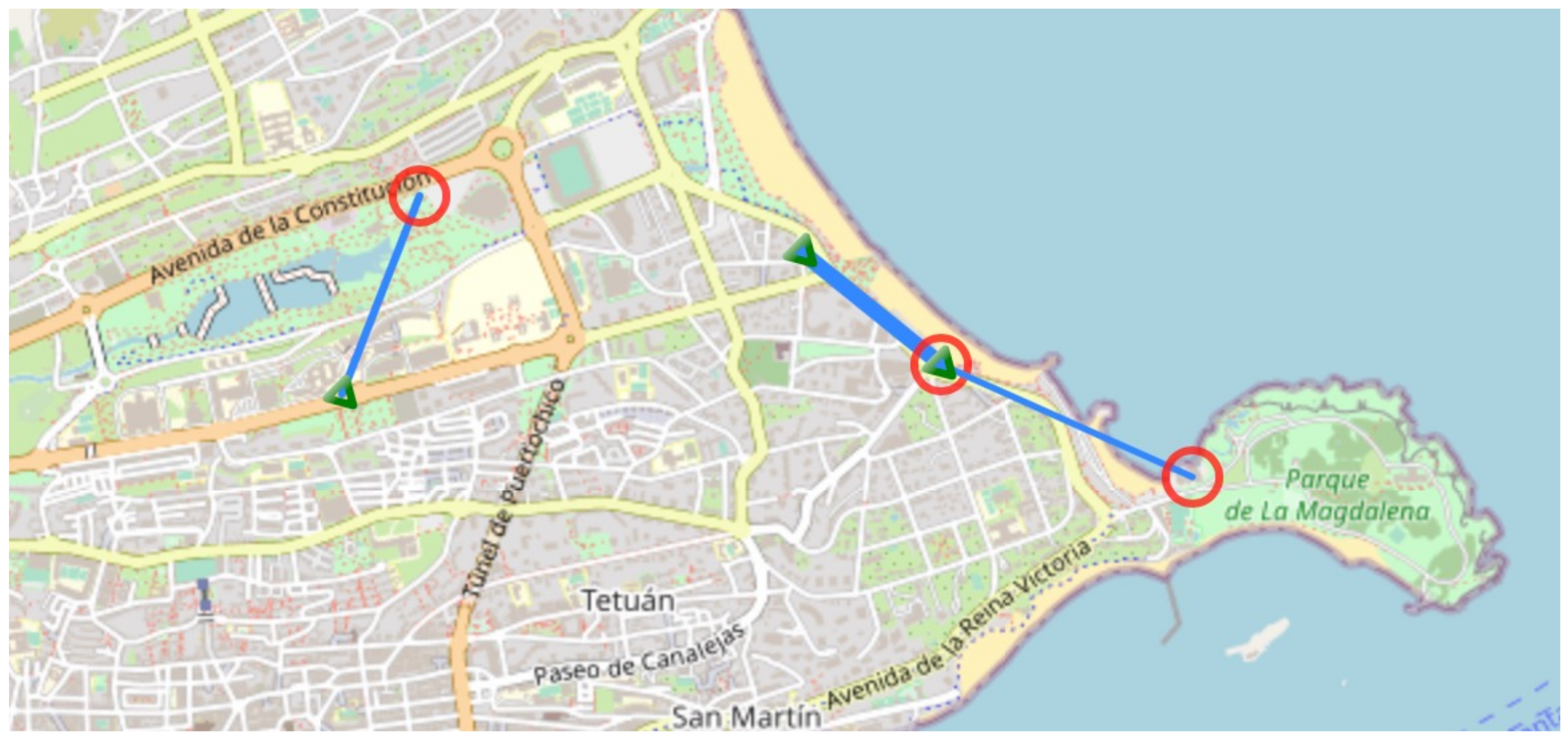
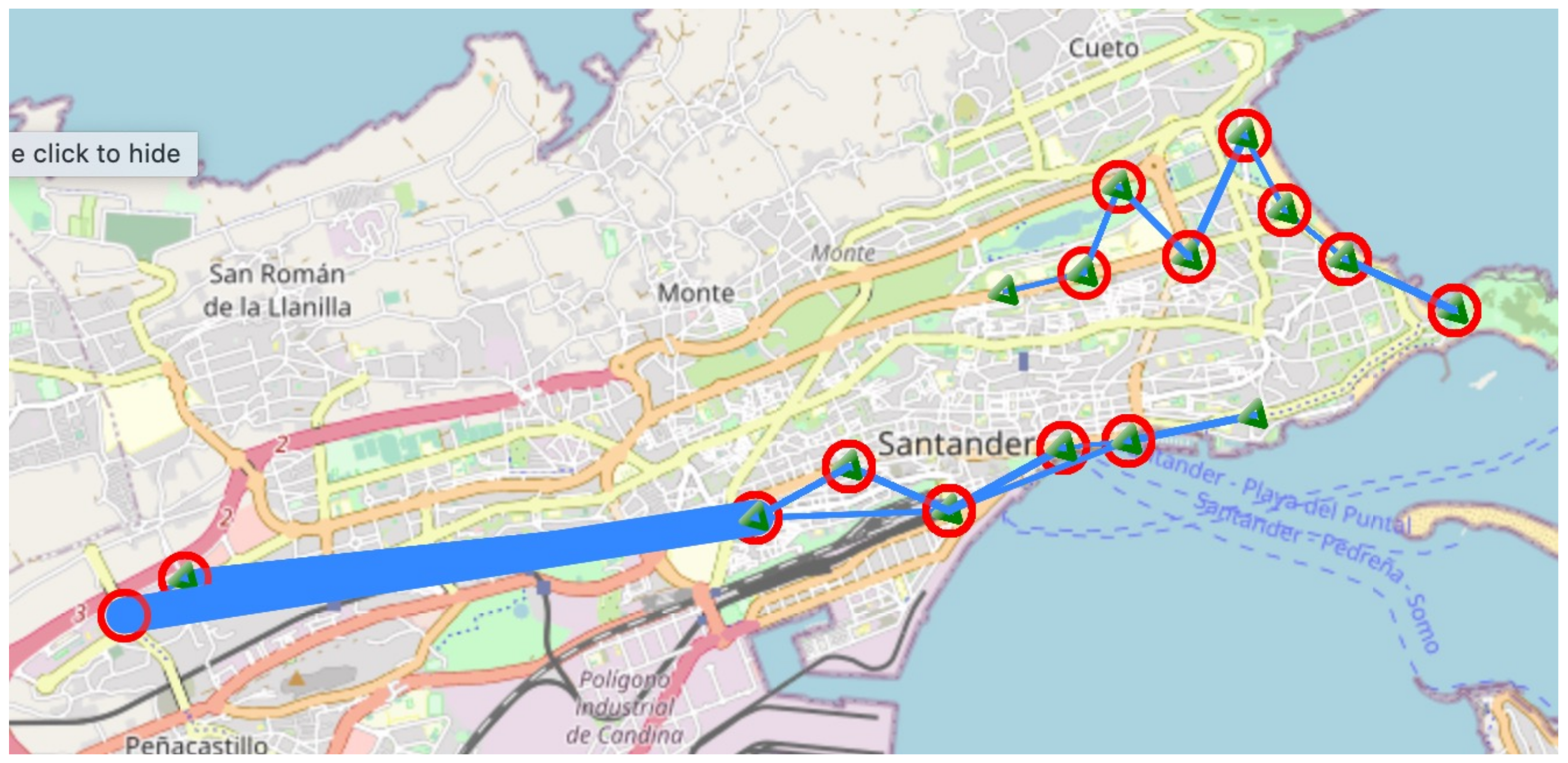
Figure 2 exhibits the trips made by users when this process is applied over a candidate solution different from the original one. Red circles stand for the origin station, blue triangles stand for the target station, and the thickness of the line is proportional to the number of users that have performed the trip. Sometimes stations may serve as origin and destination in different moments of the simulation process, stating the weakness of the areas that lack docking stations or bikes, depending on the case.
As named in the previous section, the proposed measure of the performance of a distribution of docks over a set of predefined stations in a BSS is based on total capacity (cost) and user satisfaction (amount of extra kilometers).
Regarding capacity usage, we consider the total spare capacity as the percentage of non needed docks in a BSS, calculated as the ratio of non-used docks in the case all bikes were are located at stations.
Total capacity, , is the sum of all station capacities for the candidate solution. Total bikes number is known by the institutions managing the BSS but is not directly provided by data. This constant is calculated using the number of docks used on the real case in the higher moment of occupation. As some of the users may be moving in the chosen instant, traveling from one station to other, a percentage of security measured is added to prevent the possibility of not having enough docks available for all the bikes present in the real case.
Both parameters are independent from time, and they can be calculated at once when data are extracted and applied to every candidate solution evaluation.
2.4. Measuring the System Performance Based on a Real Usage
As expressed in Equation (3), the real occupation matrix () is transformed into a matrix of requests to be applied over a different capacity distribution. The real case is usually also known as base case and we will use it interchangeably.
The fitness measured in (Equation (5)), applied over , will not generate any measure of user satisfaction (no extra kilometers) because each request was attended in ; therefore, there is no failed request information recorded.
Although we might guess that some users were not attended to, even if we do not have the proof or evidence to ensure it, we argue that failed requests are prone to happen when a station is full and a user requests an empty dock or vice-versa, when a station is empty and a user request a bike.
To highlight these effects, we propose the use of trends of , named as virtual movements (), to model the probability of a failed request happening, even in . The average quantity of these stations may predict the future demand on them, e.g., if one station i becomes full () at a given moment j, in the probability of it being similar is pretty large. Trends are calculated in a time window (V) over station movements at time j as the average of the last V movements when the station becomes full or empty and becomes zero.
’s are applied to the simulation in the same way as and called virtual requests. A virtual request will be applied to calculate extra kilometers (named virtual extra kilometers) in the same way as (see Algorithm 1) but will not change the occupation of the stations because this would change the number of total bikes in the system. Thus, this concept looks after the inertia of to predict future demands but does not change the occupation when applied.
Based on (Equation (10)), each is used as a virtual request made at a certain time to obtain or park a bike in a specific station and evaluated by Algorithm 1.
Pondering these pieces, , and , the global measure criterion can be summarized as a fitness function (Equation (11)); a function that expresses the wellness of the proposed capacity distribution in terms of capacity cost and user satisfaction:
2.5. Behavior of a Candidate Solution BSS
Simulations offer the chance to evaluate a possible scenario (candidate solution) without the inherent costs of physical implementation or a prototype; while the simulation is beingn executed, some indicators can be recorded that could help decision makers to understand the differences between various candidate solutions.
The simulation of requests over a BSS is measured mainly in this paper through the distance the user has to travel (Equations (4) and (10)); however, the number of failed requests is also per se a valuable indicator of the performance of the candidate solution. The number of times a station becomes empty or full is also useful information because this situation indicates a possible point of improvement in the network by dynamically managing the number of moving bikes from some stations to others or as a measure of strength between similar candidate solutions.
Apropos of the evaluation of user satisfaction, the number of kilometers may be described in more detail, breaking up total kilometers into two separated indicators: firstly, those performed due to a failed request of a bike, because they are made by foot, and those performed due to a failed request of a dock, which will be recorded by bike. These two indicators also inform about differences between candidate solutions in the ability of serving bikes or docks.
The analysis of a simulation over the original distribution may serve as an analysis tool to detect future improvements. For example, a stress factor can be introduced to multiply by a factor the number of requests and predict where the capacity has to be reinforced but does not propose a better distribution with the help of the named indicators; some examples will be described in the results section on the convenience of these indicators to compare different solutions.
2.6. Optimization Based on Candidate Solutions
The simulation of a candidate solution in BSS means applying some inputs (bike or dock requests) over a distribution of capacities, . This is a standard process of improvement validation over existing infrastructures in traffic and urban design [24], but it also operates as the building block for one of the most powerful optimization strategies: genetic algorithms and local searches. As far as we are able to obtain a numerical value to a candidate solution, we may compare it with other ones to minimize or maximize depending on our goals. We can guide these changes between different proposals using expert knowledge and improve the details in trying to understand the system behavior upon those changes. However, sometimes the combinatorial nature of problems and non-evident relation between parts of the solution may not help this discovery process. Optimization algorithms do not rely on knowledge and can drive the problem to a space solution search where the target is the minimum/maximum value for the candidate solution.
The candidate solution is defined in this problem as , regardless of whether the number of docks per station differs from the original but the number of stations remains the same, that is, we will not create nor remove any existing station. As the minimum size for a station capacity is not restricted, except for being greater or equal to zero, the optimization could in fact remove all activity onto a station by setting the capacity to zero. Candidate-based optimization algorithms need an evaluation function, named in this work as Fitness (Equation (11)), and some way of generating new valid candidates that may improve previously generated candidates once evaluated.
The candidate solution must be valid from the point of view of the network definition; therefore, capacity modifications cannot be made with full degrees of freedom. There is a (minimum of) fixed number of bikes (, Equation (8)), and therefore, total capacity () cannot be smaller than this number because each bike has to have at least a dock to be allocated by definition.
Optimization algorithms based on candidate solutions are based on a proper equilibrium between exploration and exploitation. In the next sections, we will consider the usage of several related algorithms that will be compared later in the results section in order to observe the computation effort versus stability and the quality of the results.
2.6.1. Best Improvement Local Search
A local search algorithm [25] considers the optimization as a search space defined by the possible variations of the elements in a candidate solution. The local optimality is achieved by local perturbations. This operation is called neighbor generation in most of the local search varieties. The inner component of the candidate solutions in the BSS problem is station capacities. As each (station capacity) can have values from 0 to n (not restricted, by definition), the neighbor generation can be made by the addition or subtraction of a number of .
These two parameters (percentage of positions to be modified (pp) and maximum amount to be added () to the selected stations) define the capacity of exploration in a hill-climbing local search (see Algorithm 1).
| Algorithm 1: Best Improvement Local Search | |
| 1 | function LocalSearch (base_case,neighbor_number): |
| 2 | Best_solution = generateNeighbor (base_case,%pp,max_am) |
| 3 | Best_fitness = Fitness (Best_Solution) |
| 4 | While not Stop_Criteria: |
| 5 | Best_neighbor = GetBestneighbor (number_of_neighbors,Best_Solution) |
| 6 | If fitness (Best_neighbor) < Best_fitness: |
| 7 | Best_fitness = fitness (Best_neighbor) |
| 8 | Best_solution = Best_neighbor |
| 9 | return Best_solution |
The initial point in our algorithm proposal is the , but it could be initialized with any valid solution. Regarding the other parameters, the number of neighbors generated in each iteration express the depth of the search by a randomized generation of neighbor instead of an exhaustive loop with the length of the neighbor generation operator defined by pp and ; Stop Criteria is based on a given number of iterations without improvements on the best solution. The combination of these two parameters allows flexible management of exploitation and exploration in the local search.
2.6.2. Variable Neighborhood Local Search
Best Improvement Local Search is based on a neighbor generation function with a fixed range (number of changes made over the given candidate). These algorithms are good enough to test the fitness function, valid candidates and the validation of the concept but has a poor exploration power depending on input parameters pp and . Thus, Variable Neighborhood Search [26] is proposed as an improvement to fix the local range search, keeping the same function for neighbor generation used in the Best Improvement Local Search. This variation has a function, VNSNeighbor, that increases the number of positions changed in one single neighbor generation every time the Best Improvement Local Search stagnates. This variable range in the operator of neighbor generation provides a way of escaping from local optima, allowing more exploration power to the search without losing exploitation due to the dynamic reduction of the range k once a new local optimum is found. The algorithm ends once the max range is reached without improvements in the best solution (Algorithm 2).
| Algorithm 2: Variable Neighborhood Local Search | |
| 1 | function VNS (base_case,neighbor_number,max_range): |
| 2 | Best_solution = generateNeighbor(base_case) |
| 3 | Best fitness = simulation(Best_Solution) |
| 4 | K = 0 |
| 5 | While K < max_range |
| 6 | Candidate = VNSneighbor(K, Best Solution) |
| 7 | Local_Search_Solution = LocalSearch(Candidate, neighbor_number) |
| 8 | If simulation (Local_Search_Solution) < Best_fitness |
| 9 | Best_fitness = simulation (Local_Search_Solution) |
| 10 | Best_solution = Local_Search_Solution |
| 11 | K = 0 |
| 12 | Else K++ |
| 13 | return Best_solution |
2.6.3. Genetic Algorithms
Genetic algorithms are population-based algorithms [27] widely used for BSS problem optimization. Some recent examples of related problems in genetic algorithms and local searches in vehicle networks can be seen in [28,29]. These algorithms use an evolution paradigm to select the best candidates (named as chromosomes) of the population and mix their positions (named as genes) in a crossover and perform neighbor-like operations (named as mutation here). The capacity distribution of each station may be seen as the genes that will be mixed over generations to create solutions that bring not just variations over previous solutions but completely new ones with the better genes of their parents. A local search can be seen as a trajectory over a search space with the movement capacity of the neighbor operator, but genetic algorithms break this view by a building block theory in which a better combination will remain in the population in the form of genes and statistically will guide the selection and build even better structures. The results of this operation are offsprings (candidate solutions) that will remain in the population over time if they are better than other individuals.
Genetic algorithms are able to explore complicated combinatorial problems if the equilibrium between genetic diversity and selection pressure keeps the key genes improving without falling in a local optimum because of a lack of diversity in the population.
Best Improvement Local Search, VNS and Genetic Algorithm share the same codification for mutation (named neighbor generation in the local search) and fitness evaluation.
The genetic algorithm proposed can be outlined as a loop where in every iteration two individuals are selected by tournament selection [30], selecting the best individual from a random sampling of size k. The mutation operator makes the system explore outside the initial values of the genes present in the population. This operator is the same one used in the Best Improvement Local Search, named there as neighbor generation. The key operation in the generation and improvement of new individuals is Crossover [31]. This operator is applied over two elements and mutated to create new solutions that may have a better value once evaluated. Crossover selects two points that crossover; this one may generate invalid chromosomes due to restrictions on the minimum capacity, preventing some bikes from finding an available dock; to avoid this issue, two random positions are selected, and the list of positions is copied on the offsprings bearing in mind not to be below the minimal capacity of the factor.
It may happen that after copying the fragment, the resultant offspring may be invalid due to the total capacity of the network being lower than the number of bikes. To fix the chromosome, the following positions will be copied until this criterion (capacity greater or equal than bike number) is fulfilled. No max (Total capacity) restriction has been set for the sake of clarity.
Let us see an example: being two candidates of a city with eight stations and 100 bikes: and , the crossover will produce the following results: random positions , . . This offspring is invalid due to the total capacity being lower than the number of bikes (58). The algorithm will then extend the copied positions until it is valid on position 5, being the result Offspring1 = [15, 2, 4, 40, 25, 30]. The number of individuals in the population is fixed, therefore these two solutions will replace some other one using a steady state population type [32]. To increase the genetic pressure in a flexible way, these two offsprings will replace two individuals from the population using tournament replacement [33], where the selected ones are the worst element of a random set of size k. This strategy promotes the probabilities of poor elements of being deleted and good elements to remain in the pool.
Finally, we propose a Hybrid Genetic Algorithm 3 with a local search as the better approach for this optimization problem, thanks to the good capability of local search algorithms to improve a good solution and the exploration capacity of the genetic search. These hybrid heuristics, which combine concepts and strategies applied by other metaheuristics such as population-based search and local search, are similar to Memetic Algorithms [34,35]. The main difference between the proposed Hybrid genetic algorithm and the Memetic Algorithms is the fact that in Memetic algorithms [36] in any generation, the population of individuals consists solely of local optima, and in the Hybrid Algorithm proposed, the added local search only runs every certain number of iterations, reinforcing that closer minimums to the optima finally become optimized to the optima. This approach provides more time for the algorithm to explore the space before stagnation.
| Algorithm 3: Hybrid Genetic Algorithm | |
| 1 | function Hybrid Genetic (base_case,neighbor_number,number_iterations): |
| 2 | Best solution = (base case) |
| 3 | Best fitness = simulation(Best Solution) |
| 4 | Generate Population (as Strong mutation of base case) |
| 5 | While not Stop_Criteria: |
| 6 | S1 = Mutation (Crossover(Selection(Population , k))) |
| 7 | If fitness (S1) < Best_fitness: |
| 8 | Best_fitness = fitness (S1) |
| 9 | Best_solution = S1 |
| 10 | Population = replace (S1 , k) |
| 11 | Every (number_iterations): |
| 12 | Best_solution = localSearch (Best_Solution , neighbor_number)} |
| 13 | return Best_solution |
2.7. Use Case: Santander Bike Sharing System
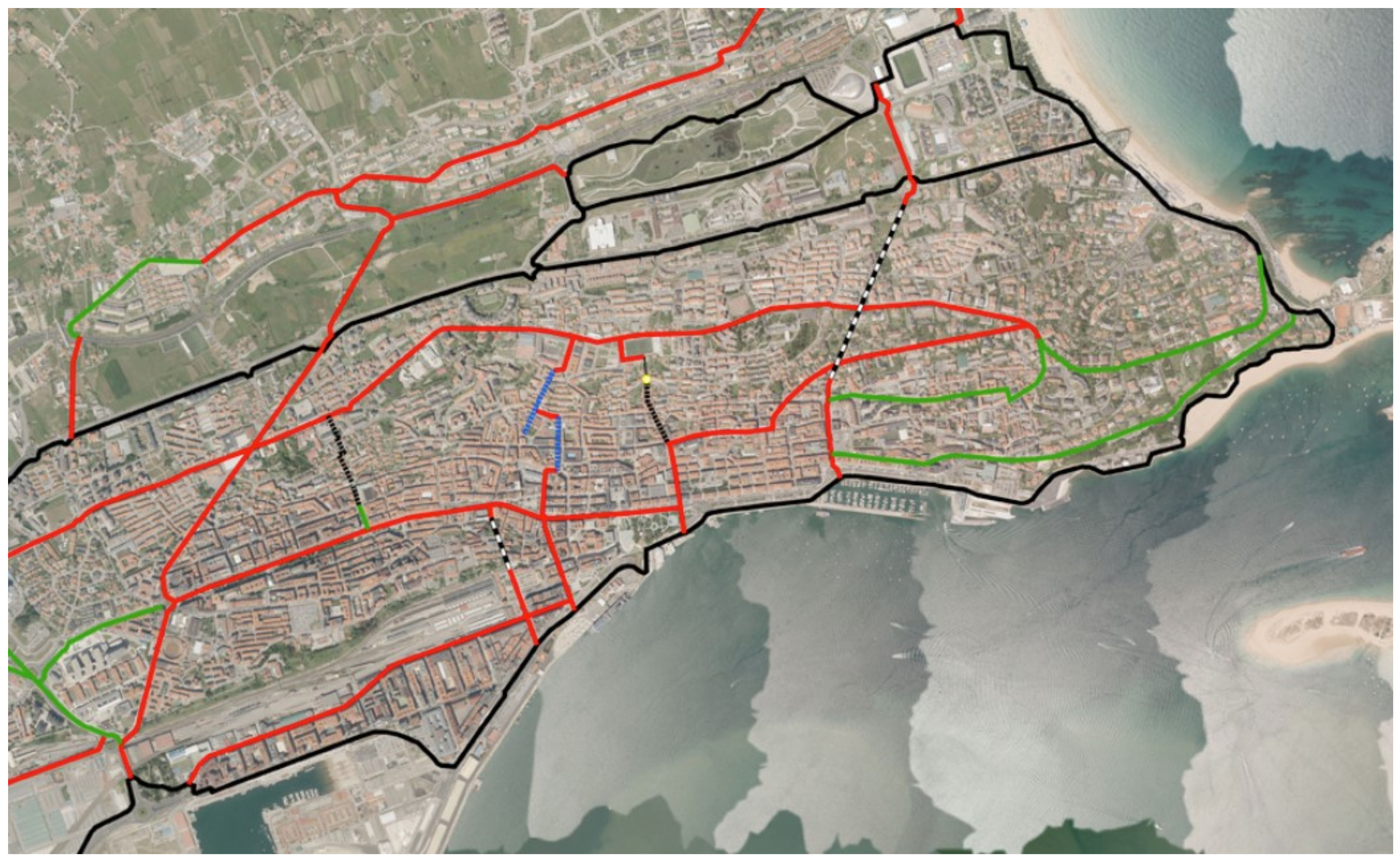
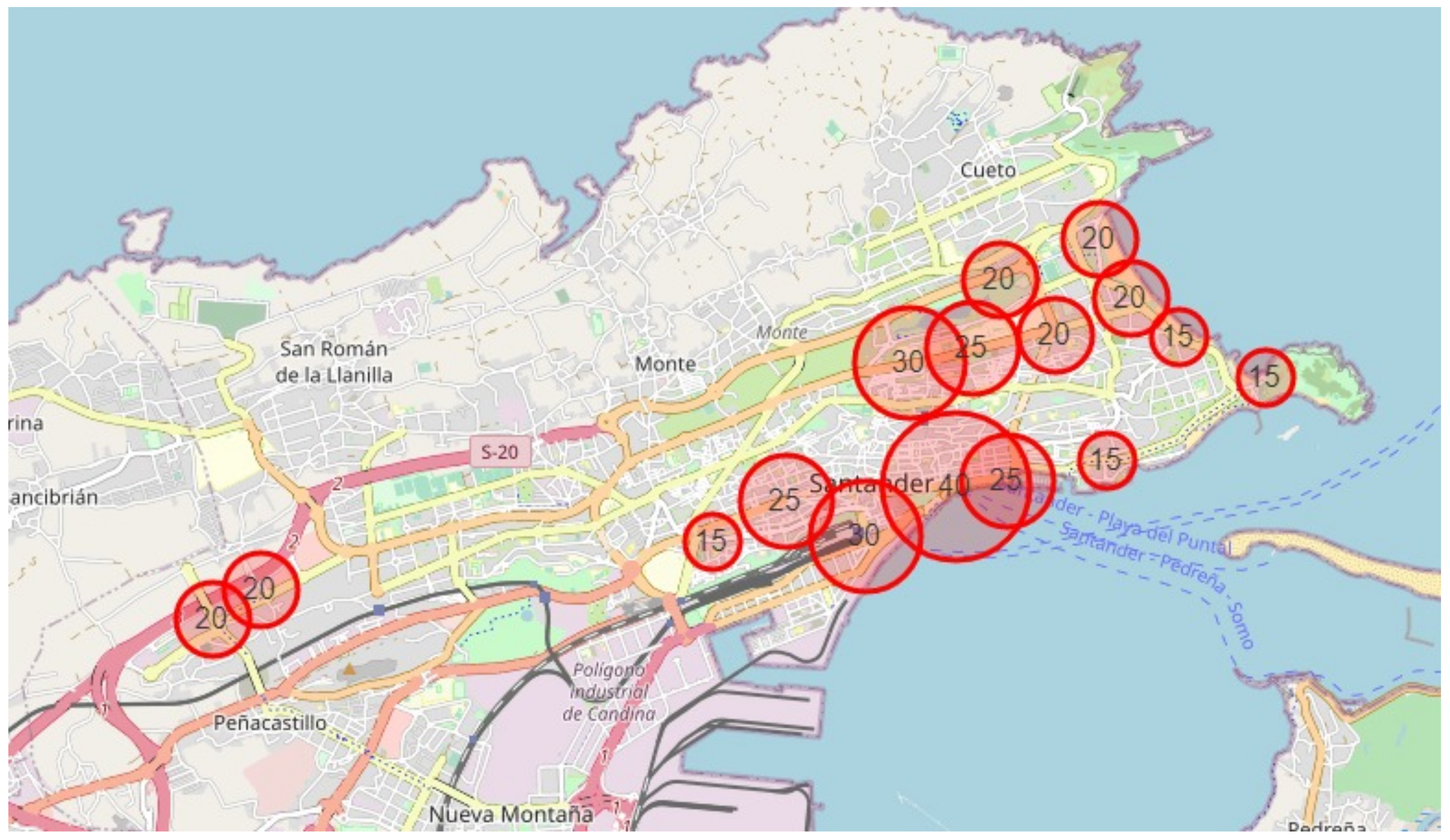
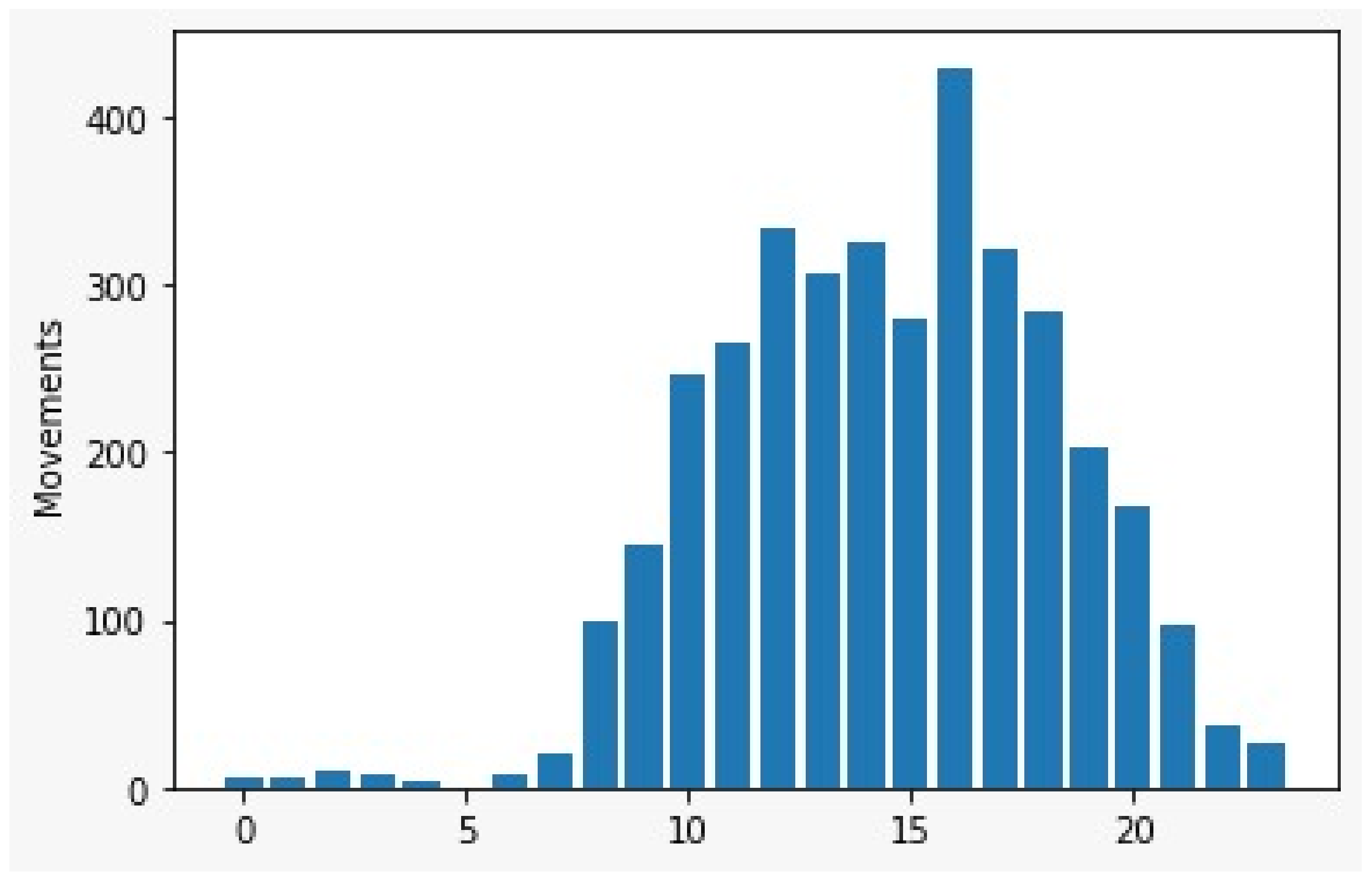
This proposal handles the simulation of a real BSS based on the Santander BSS (Spain) as a representative case for validating some of the measures and techniques proposed in this work. Santander has a small network of 16 stations with clear and differentiated areas: on the left the industrial area, down in the middle the train station, in the inner part some residential areas and lastly the coast and downtown, down and on the right, respectively. It is a city with no rivers and short distances that ease the calculus extrapolation because each direction is equally probable in terms of user eligibility. It has a network of dedicated paths for bikes 18 kms length in total, where most of the stations are situated along the route, making the riding safer (Figure 3). The size of the city and the small number of stations are within the preferred criteria for testing, being able to understand the results and extrapolate conclusions keeping the complexity of the problem high enough to overcome direct combination optimization. Concerning the size of the stations, (Figure 4), the average size is around 20 docks per station, with some doubling this quantity with a total capacity of 355 docks and a total number of bikes in the system of 198.
Each station is located at a certain position given by its latitude and longitude coordinates and has a potentially different number of docks with a set of available docks at a certain time of the day.
We propose the use of real data in a simulation to measure changes in the capacity distribution. In this setting, Santander has a mild climate with minor variability between seasons. Ideally, several years of data could be used to ensure proper support to all the cases, but for the sake of performance, we have evaluated the most demanding months of the year and compared this period between years from 2017 to 2020. The month with less variability between years and more accumulated usage per day was April 2019. This month has the most demanding average usage per hour. Figure 5 shows the accumulated requests in the network by hour. We have paid special attention to critical situations as to whether some of the stations become full or empty and the probability of movements on those stations remains high.
3. Results
The experimentation was executed for the four exposed algorithms; Best Improvement Local Search (BL), Variable Neighborhood Search (VNS), Genetic Algorithm (GA) and Hybrid Genetic Algorithm (HGA). Each algorithm was executed with 10 seeds for the dataset, showing the best results for each set of executions.
Metaheuristic optimization has a considerable number of parameters that may impact on the quality of the solution and the time of execution. Initial experimentation with BL and VNS using grid hyperparameter tuning [37] was performed to determine the better values of the parameters. The Best Improvement Local Search is shown in Table 2.
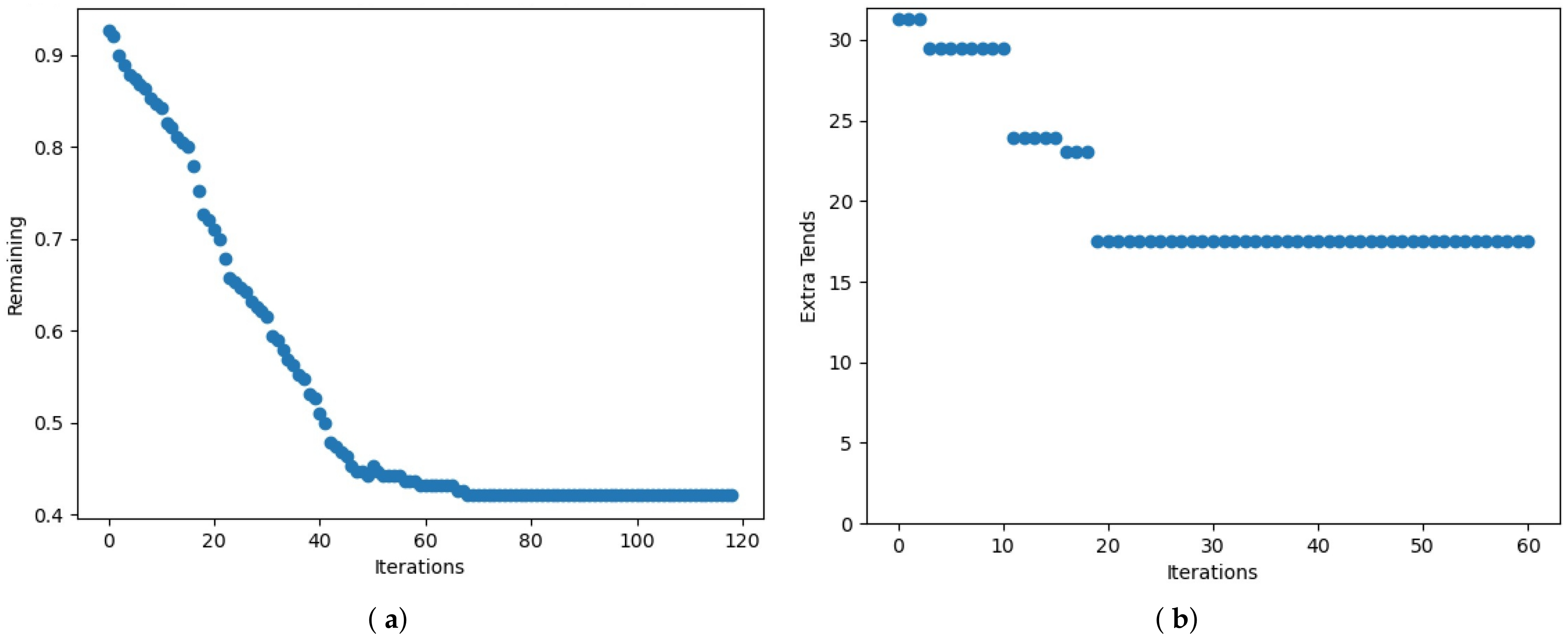
Both BL and VNS show an adequate convergence to the optima, Figure 6 shows the behavior of the two parts of the fit: total spare capacity (a) and the extra virtual kilometers (b) of the best individual within the BL optimization.
Based on the Local Search parameter tuning, we have better results for genetic and hybrid algorithms, adding the additional parameters shown in Table 3.
The problem chosen for this optimization has been solved in some of the executions by all the optimization algorithms proposed, even if the total number of combinations is bigger than (). The evaluation of a single solution may take around half a second using a one-week interval, which gives a time of more than seven days of computation to arrive at the optima visiting all possible combinations compared to a much lower execution time of the proposed algorithms, as can be seen in Table 4.
BL already obtained the optima, so VNS, GA and HGA return the same individual in some of the executions. The optima for this problem in the chosen time frame is 22.16 corresponding to . The only difference between them is stability and execution time. Meanwhile, BL and VNS obtain the optima 53% and 75% of the time, respectively, the Genetic Algorithm arrives at the optima 97% and Genetic Hybrid Algorithms 100% of the time. Execution time is much higher in VNS than the other algorithms. The Genetic Algorithm shows a good performance regarding the quality of the solution and the reliability of the algorithm with the lower execution time, whereas the Hybrid Genetic Algorithm has the better reliability finding the optima for this problem 100% of the time at the expense of an execution time that nearly doubles the Genetic Algorithm. Table 4 shows averaged and standard deviation for time (minutes), evaluations, percentage of times the optima has been found and fitness.
Table 5 shows the comparison between the base case, the optimized one with capacity optimization (OP), without capacity optimization (OP_NC, i.e., only dock reallocation between stations, total capacity remains the same) and with an extra 10% of movements than the original to represent the stress of adding new users (OP_ST). The capacity column expresses the total number of docks in the network, represents total real kilometers, is the total virtual kilometers, is the percentage of empty places relative to the number of bikes, full and empty for the number of times one station achieves this state within the simulation, and finally, fitness (Equation (11)).
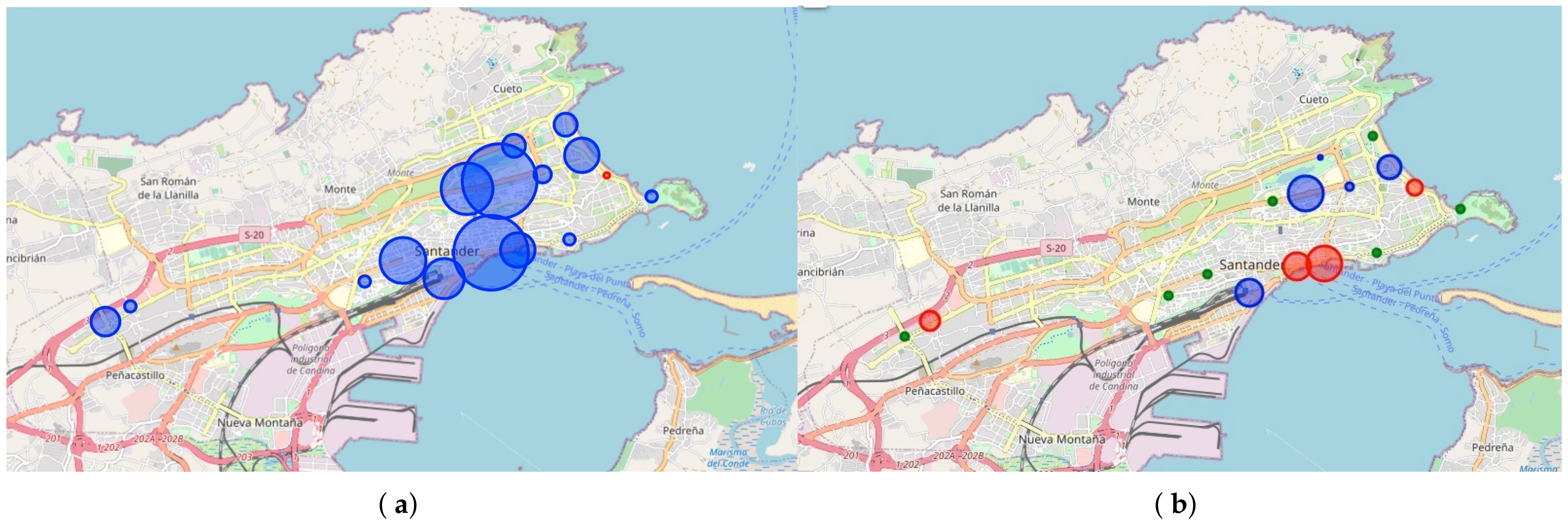
The comparison between the optimized solution and the initial one shows that with a much lower capacity, the system is able to obtain better results, increasing the real kilometers by just 0.46 kms but decreasing the number of virtual movements from 28.87 to 17.49 kms. This result denotes a user satisfaction increase of 10.92 kms against . Figure 7 shows the decrease in capacity of the majority of the stations and the increase in station #1.
With the reallocation of bikes from some stations to others (0.46 kms), produced by lowering the capacity of some stations, the algorithm has lowered the number of empty stations from 23 to 11. This optimization cannot improve this number without adding more bikes to the systems, and this is out of the scope of the algorithm. Notice that as predicted in the previous section, does not produce real extra kilometers because what was recorded were successful requests.
From the point of view of the behavior indicators stated in Table 6, it shows failed requests as the exact number of requests that are not attended. Those can be virtual or real ones. Input kilometers are those generated as a result of a failed request of requesting a bike at an empty station, and output kilometers are created by a dock request at a full station that could not be served. Base () shows a big number of failed requests all due to requests of bikes at empty stations. Even if the reasonable outcome will be to increment the number of bikes at those stations, by dynamical movements or just increasing the total number of bikes, a look at the OP and OP_NC shows that with some minor extra kilometers (3.68 kms by bike) due to not attending dock requests, the number of failed requests is much lower (13) and the output kilometers are just 13.80. OP_ST shows that even increasing the number of movements by 10%, a smaller distribution capacity is able to achieve fewer failed requests and fewer extra kilometers.
Regarding the behavior under modified conditions, some simulation has been performed over the optimized solution with changes in the number of . We have stressed the number of requests by 10%, obtaining the results in Figure 8. This is not the same as the result shown in Table 5 with OP_ST; this one exhibits the evaluation of the optimized solution with capacity change (OP) measured with the stressed . As can be observed in this figure, the optimization capacity over-fits the current usage, with a great impact on real kilometers when some extra movements are applied. The solution to predict future behavior is to optimize (OP_ST) with the stressed movements, with an increase of just 5.16 kms. An interesting result is that the number of full stations decreases, so more movement is not always a reason for a shortage of places because the interaction between negative and positive movements are not easy to predict when the users are reallocated to the nearby stations.
4. Conclusions
The simulation based on recorded requests of real usage over an alternative capacity distribution offers a useful tool to understand BSS behavior. Nevertheless, a set of variables and measures is needed to compare performance and behavior between several capacity configurations.
From the point of view of behavior interpretation, a set of markers has been defined, such as the number of times stations become full/empty, giving an overview of the peaks in the BSS, number of failed requests, input and output kilometers, which makes the results easy to understand. Furthermore, Figure 2 and Figure 8, with the specific routes performed by the user with failed requests, help to predict future behavior and assist experts on specific improvements on the network.
On the standardized performance of BSS, two facets are considered; on the one hand, user satisfaction defined as the number of kilometers pursued in the alternative distribution and, on the other hand, the cost of the infrastructure as the total capacity of the BSS.
This simulation process can also serve as a fitness function for optimization algorithms based on candidate solutions. This work has proposed an effective methodology to implement a set of optimization algorithms over existing BSS capacity records that create a better distribution capacity to increase user satisfaction and minimize the total cost by reducing the capacity of the BSS. The Hybrid Genetic Algorithm has proven to be the most reliable algorithm with a reasonable execution time.
The case of Santander BSS was selected for its implicit characteristics without geographical barriers, distribution on inner stations and mild climate that may reflect an average behavior in the usage of any of the stations at any time of the year. The results show a clear user satisfaction increase by lowering the number of kilometers and also a lower number of docks needed in the BSS. This dataset has been chosen as a first study case over the main optimization criteria for BSS networks. In future works, we will use bigger datasets and compare results considering other variables as physical barriers or station distribution.
Author Contributions
All authors contributed equally to this work. All authors have read and agreed to the published version of the manuscript.
Funding
This research is funded by FEDER 2014–2020, Junta de Andalucía and Universidad de Huelva, project UHU-1266216 and the Ministerio Español de Economía y Competitividad, projects TIN2017-85727-C4-2-P (UGR-DeepBio) and PID2020-115570GB-C22 (DemocratAI::UGR).
Institutional Review Board Statement
Not applicable.
Informed Consent Statement
Not applicable.
Data Availability Statement
Source data is available at https://zenodo.org/record/5485072, accessed on 31 July 2021.
Acknowledgments
University of Huelva and University of Granada.
Conflicts of Interest
The authors declare no conflict of interest.
References
- Fishman, E. Bikeshare: A Review of Recent Literature. Transp. Rev. 2016, 36, 92–113. [Google Scholar] [CrossRef]
- Soriguera, F.; Casado, V.; Jiménez, E. A simulation model for public bike-sharing systems. Transp. Res. Procedia 2018, 33, 139–146. [Google Scholar] [CrossRef]
- Mi, Z. Environmental benefits of bike sharing: A big data-based analysis. Appl. Energy 2018, 220, 296–301. [Google Scholar]
- Fuller, G.; Waitt, G.; Buchanan, I.; Ozolins, N. The Problem Isn’t Dockless Share Bikes. It’s the Lack of Bike Parking. 2018. Available online: https://theconversation.com/ (accessed on 3 September 2021).
- Midgley, P. The role of smart bike-sharing systems in urban mobility. Journeys 2009, 1, 23–31. [Google Scholar]
- Sun, Y. Sharing and Riding: How the Dockless Bike Sharing Scheme in China Shapes the City. Urban Sci. 2018, 2, 68. [Google Scholar] [CrossRef] [Green Version]
- DeMaio, P. Bike-sharing: History, impacts, models of provision, and future. J. Public Transp. 2009, 12, 3. [Google Scholar] [CrossRef]
- Maioli, H.C.; Carvalho, R.; Medeiros, D.D. SERVBIKE: Riding customer satisfaction of bicycle sharing service. Sustain. Cities Soc. 2019, 50, 101680. [Google Scholar] [CrossRef]
- Mattson, J.; Godavarthy, R. Bike Share in Fargo, North Dakota: Keys to Success and Factors Affecting Ridership. Sustain. Cities Soc. 2017, 34. [Google Scholar] [CrossRef]
- Pfrommer, J.; Warrington, J.; Schildbach, G.; Morari, M. Dynamic Vehicle Redistribution and Online Price Incentives in Shared Mobility Systems. IEEE Trans. Intell. Transp. Syst. 2014, 15, 1567–1578. [Google Scholar] [CrossRef] [Green Version]
- Benchimol, M.; Benchimol, P.; Chappert, B.; de la Taille, A.; Laroche, F.; Meunier, F.; Robinet, L. Balancing the stations of a self service “bike hire” system. RAIRO-Oper. Res.-Rech. Oper. 2011, 45, 37–61. [Google Scholar] [CrossRef]
- Shui, C.; Szeto, W. A review of bicycle-sharing service planning problems. Transp. Res. Part Emerg. Technol. 2020, 117, 102648. [Google Scholar] [CrossRef]
- Sayarshad, H.; Tavassoli, S.; Zhao, F. A multi-periodic optimization formulation for bike planning and bike utilization. Appl. Math. Model. 2012, 36, 4944–4951. [Google Scholar] [CrossRef]
- Lin, J.R.; Yang, T.H. Strategic design of public bicycle sharing systems with service level constraints. Transp. Res. Part E Logist. Transp. Rev. 2011, 47, 284–294. [Google Scholar] [CrossRef]
- Guo, T.Y.; Zhang, P.; Shao, F.; Liu, Y.S. Allocation optimization of bicycle-sharing stations at scenic spots. J. Cent. South Univ. 2014, 21, 3396–3403. [Google Scholar] [CrossRef]
- Corcoran, J.; Li, T.; Rohde, D.; Charles-Edwards, E.; Mateo-Babiano, D. Spatio-temporal patterns of a Public Bicycle Sharing Program: The effect of weather and calendar events. J. Transp. Geogr. 2014, 41, 292–305. [Google Scholar] [CrossRef]
- Froehlich, J.; Neumann, J.; Oliver, N. Sensing and Predicting the Pulse of the City through Shared Bicycling. In Proceedings of the 21st International Jont Conference on Artifical Intelligence, IJCAI’09, Pasadena, CA, USA, 11–17 July 2009; Morgan Kaufmann Publishers Inc.: San Francisco, CA, USA, 2009; pp. 1420–1426. [Google Scholar]
- Han, Y.; Côme, E.; Oukhellou, L. Toward Bicycle Demand Prediction of Large-Scale Bicycle-Sharing System. In Proceedings of the Transportation Research Board 93rd Annual Meeting, Washington, DC, USA, 12–16 January 2014. [Google Scholar]
- Caggiani, L.; Camporeale, R.; Marinelli, M.; Ottomanelli, M. User satisfaction based model for resource allocation in bike-sharing systems. Transp. Policy 2019, 80, 117–126. [Google Scholar] [CrossRef]
- Fricker, C.; Gast, N.; Mohamed, H. Mean field analysis for inhomogeneous bike sharing systems. In Proceedings of the 23rd International Meeting on Probabilistic, Combinatorial, and Asymptotic Methods for the Analysis of Algorithms, Montreal, QC, Canada, 18–22 June 2012. [Google Scholar]
- Alvarez-Valdes, R.; Belenguer, J.M.; Benavent, E.; Bermudez, J.D.; Muñoz, F.; Vercher, E.; Verdejo, F. Optimizing the level of service quality of a bike-sharing system. Omega 2016, 62, 163–175. [Google Scholar] [CrossRef]
- Caggiani, L.; Ottomanelli, M. A Modular Soft Computing based Method for Vehicles Repositioning in Bike-sharing Systems. Procedia-Soc. Behav. Sci. 2012, 54, 675–684. [Google Scholar] [CrossRef] [Green Version]
- JCDecaux. JCDecaux Developer. Open Data. 2021. Available online: https://developer.jcdecaux.com/ (accessed on 3 September 2021).
- American Planning Association. Planning and Urban Design Standards; John Wiley & Sons: Hoboken, NJ, USA, 2006. [Google Scholar]
- Johnson, D.S.; Papadimitriou, C.H.; Yannakakis, M. How easy is local search? J. Comput. Syst. Sci. 1988, 37, 79–100. [Google Scholar] [CrossRef] [Green Version]
- Hansen, P.; Mladenović, N. Variable neighborhood search. In Handbook of Metaheuristics; Springer: Berlin/Heidelberg, Germany, 2003; pp. 145–184. [Google Scholar]
- Liu, J.; Li, Q.; Qu, M.; Chen, W.; Yang, J.; Xiong, H.; Zhong, H.; Fu, Y. Station site optimization in bike sharing systems. In Proceedings of the 2015 IEEE International Conference on Data Mining, Atlantic City, NJ, USA, 14–17 November 2015; pp. 883–888. [Google Scholar]
- Long, J.; Sun, Z.; Pardalos, P.M.; Hong, Y.; Zhang, S.; Li, C. A hybrid multi-objective genetic local search algorithm for the prize-collecting vehicle routing problem. Inf. Sci. 2019, 478, 40–61. [Google Scholar] [CrossRef]
- Verma, A. Electric vehicle routing problem with time windows, recharging stations and battery swapping stations. EURO J. Transp. Logist. 2018, 7, 415–451. [Google Scholar] [CrossRef]
- Miller, B.L.; Goldberg, D.E. Genetic algorithms, tournament selection, and the effects of noise. Complex Syst. 1995, 9, 193–212. [Google Scholar]
- Spears, W.M. Adapting crossover in evolutionary algorithms. In Proceedings of the 4th Annual Conference on Evolutionary Programming; McDonnell, J.R., Reynolds, R.G., Fogel, D.B., Eds.; MIT Press: Cambridge, UK, 1995; pp. 367–384. [Google Scholar]
- Vavak, F.; Fogarty, T.C. Comparison of steady state and generational genetic algorithms for use in nonstationary environments. In Proceedings of the IEEE International Conference on Evolutionary Computation, Nagoya, Japan, 20–22 May 1996; pp. 192–195. [Google Scholar]
- Naoum, R.; Aziz, S.; Alabsi, F. An enhancement of the replacement steady state genetic algorithm for intrusion detection. Int. J. Adv. Comput. Res. 2014, 4, 487. [Google Scholar]
- Caraffini, F.; Neri, F.; Iacca, G.; Mol, A. Parallel memetic structures. Inf. Sci. 2013, 227, 60–82. [Google Scholar] [CrossRef]
- Caraffini, F.; Neri, F.; Picinali, L. An analysis on separability for Memetic Computing automatic design. Inf. Sci. 2014, 265, 1–22. [Google Scholar] [CrossRef]
- Merz, P.; Freisleben, B. A comparison of memetic algorithms, tabu search, and ant colonies for the quadratic assignment problem. In Proceedings of the 1999 Congress on Evolutionary Computation-CEC99 (Cat. No. 99TH8406), Washington, DC, USA, 6–9 July 1999; Volume 3, pp. 2063–2070. [Google Scholar] [CrossRef]
- Feurer, M.; Hutter, F. Hyperparameter Optimization. In Automated Machine Learning: Methods, Systems, Challenges; Springer International Publishing: Cham, Switzerland, 2019; pp. 3–33. [Google Scholar] [CrossRef] [Green Version]
Figure 1.
Request distribution and calculation of kilometers performed by users.

Figure 2.
Extra distribution of users produced in a simulation.

Figure 3.
Santander’s bike path. Black indicates already existing infrastructures.

Figure 4.
Stations and capacity distribution in Santander BSS.

Figure 5.
Movement distribution per hour in April over Santander BSS.

Figure 6.
Fitness evolution in BL: (a) Total spare capacity. (b) Kilometers extra due to trends.

Figure 7.
Station capacity delta on optimized solutions: (a) optimized solution with capacity change, (b) optimized capacity without capacity change. Blue represents decreased capacity. Red represents increased capacity and radius the amount of difference with .
Figure 7.
Station capacity delta on optimized solutions: (a) optimized solution with capacity change, (b) optimized capacity without capacity change. Blue represents decreased capacity. Red represents increased capacity and radius the amount of difference with .

Figure 8.
Extra kilometers in optimized solution, 10% of stress over movements.


Table 1.
Dataset sample.
| City | # Stat. | Capac. | Docks | Bikes | Lat. | Lon. | Date |
|---|---|---|---|---|---|---|---|
| Santander | 2 | 20 | 7 | 13 | 43.4744 | −3.7857 | 15 April 2019 11:50 |
| Santander | 4 | 20 | 10 | 10 | 43.4784 | −3.7886 | 15 April 2019 11:50 |
| Santander | 17 | 20 | 13 | 7 | 43.4548 | −3.8669 | 15 April 2019 11:50 |
| Santander | 16 | 20 | 8 | 12 | 43.4528 | −3.8713 | 15 April 2019 11:50 |
| Santander | 12 | 15 | 15 | 0 | 43.4691 | −3.7732 | 15 April 2019 11:50 |
| … |
Table 2.
Best Improvement Local Search parameters.
| Parameter | Description | Value |
|---|---|---|
| %Positions: | Position changes in every neighbor generation. | 10% |
| %Quantity: | Max number of changes to add or subtract. | 10% |
| %SpareFactor: | The weight of the empty places over user satisfaction in fitness | 10% |
| Max Epochs: | Number of times without improvement before stopping. | 20 |
| Neigbors: | Number of neighbors to be generated in each iteration | 50 |
Table 3.
Additional parameters for genetic and hybrid algorithms.
| Parameter | Description | Value |
|---|---|---|
| Population size: | Number of individuals | 30 individuals |
| Population type: | Steady state | single pop. with replacement |
| Selection operator: | Tournament selection | over 10% of pop. |
| Replacement operator: | Tournament | over 20% of pop. |
| Crossover: | Crossover operator | two points |
| Mutation: | %positions %quantity | (10% of length, 10% of station value) |
| Max Epochs: | Number of times without improvement before stopping | 20 |
| BL_Epochs: | Number generations to launch a BL in the hybrid scheme | 20 |
Table 4.
Algorithm comparison.
| # | Evaluations | St. Dev | Time | St. Dev | % Optima | Fitness | St. Dev |
|---|---|---|---|---|---|---|---|
| BL | 6800 | 925 | 28.87 | 3.3 | 53% | 22.31 | 1.70 |
| VNS | 21.099 | 2094 | 47.27 | 7.1 | 75% | 22.25 | 0.10 |
| GEN | 5034 | 589 | 26.27 | 3.6 | 97% | 22.11 | 0.04 |
| HYB | 8886 | 935 | 45.80 | 4.7 | 100% | 22.16 | 0.00 |
Table 5.
Base case vs. optimized performance, Santander.
| # | Capacity | Trk | Tvk | Spare | Full | Empty | Fitness |
|---|---|---|---|---|---|---|---|
| Base | 355 | 0.00 | 28.87 | 87 | 0 | 23 | 35.55 |
| OP | 270 | 0.46 | 17.49 | 42 | 4 | 11 | 22.16 |
| OP_NC | 355 | 0.46 | 17.49 | 87 | 4 | 11 | 26.63 |
| OP_ST | 292 | 0.71 | 22.40 | 53 | 0 | 17 | 28.48 |
Table 6.
Base case vs. optimized behavior indicators, Santander.
| # | Capacity | Trk | Tvk | Failed Requests | Input kms | Output kms |
|---|---|---|---|---|---|---|
| Base | 355 | 0.0 | 28.87 | 46 | 0 | 28.87 |
| OP | 270 | 0.46 | 17.49 | 13 | 3.68 | 13.80 |
| OP_NC | 355 | 0.46 | 17.49 | 13 | 3.68 | 13.80 |
| OP_ST | 292 | 0.71 | 22.40 | 21 | 0 | 22.40 |
Publisher’s Note: MDPI stays neutral with regard to jurisdictional claims in published maps and institutional affiliations. |
© 2021 by the authors. Licensee MDPI, Basel, Switzerland. This article is an open access article distributed under the terms and conditions of the Creative Commons Attribution (CC BY) license (https://creativecommons.org/licenses/by/4.0/).
Share and Cite
MDPI and ACS Style
Aranda-Corral, G.A.; Rodríguez, M.A.; Fernández de Viana, I.; Arenas, M.I.G. Genetic Hybrid Optimization of a Real Bike Sharing System. Mathematics 2021, 9, 2227. https://0-doi-org.brum.beds.ac.uk/10.3390/math9182227
AMA Style
Aranda-Corral GA, Rodríguez MA, Fernández de Viana I, Arenas MIG. Genetic Hybrid Optimization of a Real Bike Sharing System. Mathematics. 2021; 9(18):2227. https://0-doi-org.brum.beds.ac.uk/10.3390/math9182227
Chicago/Turabian StyleAranda-Corral, Gonzalo A., Miguel A. Rodríguez, Iñaki Fernández de Viana, and María Isabel G. Arenas. 2021. "Genetic Hybrid Optimization of a Real Bike Sharing System" Mathematics 9, no. 18: 2227. https://0-doi-org.brum.beds.ac.uk/10.3390/math9182227
Note that from the first issue of 2016, this journal uses article numbers instead of page numbers. See further details here.