G³ Shape Adjustable GHT-Bézier Developable Surfaces and Their Applications

Abstract

In this article, we proposed a novel method for the construction of generalized hybrid trigonometric (GHT-Bézier) developable surfaces to tackle the issue of modeling and shape designing in engineering. The GHT-Bézier developable surface is obtained by using the duality principle between the points and planes with GHT-Bézier curve. With different shape control parameters in their domain, a class of GHT-Bézier developable surfaces can be established (such as enveloping developable GHT-Bézier surfaces, spine curve developable GHT-Bézier surfaces, geodesic interpolating surfaces for GHT-Bézier surface and developable GHT-Bézier canal surfaces), which possess many properties of GHT-Bézier surfaces. By changing the values of shape parameters the effect on the developable surface is obvious. In addition, some useful geometric properties of GHT-Bézier developable surface and the $G^1$, $G^2$ (Farin-Boehm and Beta) and $G^3$ continuity conditions between any two GHT-Bézier developable surfaces are derived. Furthermore, various useful and representative numerical examples demonstrate the convenience and efficiency of the proposed method.

1. Introduction

Due to particular features, the theory of developable surfaces has great importance in the geometric modeling and CAD/CAM fields. A developable surface is a special kind of ruled surface that can be obtained by twisting a plane without contraction and stretching, while in differential geometry, it can be defined as a surface that has a zero Gaussian curvature at each point on it. Developable surfaces are always significant because they can be implemented in the engineering field to create numerous products such as mechanical parts, pipelines, shoe upper, aircraft wings, automobile body, clothing, and ship hulls [1,2,3,4,5]. In CAGD, the designing of developable surfaces is very common, due to the wide range of applications. The designing of developable surfaces can be made possible in two ways—by the point geometry representation method and by interpolation of any two boundary curves [2,3]. In the case of point geometry representation, the developable surface has the same properties as seen in the tensor product surface. There are two other methods for the implementation of the point geometry representation method. One is the designing of the developable surface by original direction and given directrix and the other is by interpolation of any two boundary curves. The second approach is the geometrical representation, by plane and line, used for designing developable surfaces.

The three basic representations of a developable surface are cone, cylinder, and the tangent surface of a curve. The fabrication and local shape adjustment of generalized developable cubic trigonometric Bézier (GDCT-Bézier) surface with shape parameters is presented by Ammad et al. [4]. Various modeling examples with continuity conditions between two developable surfaces are also described. Hu et al. [6], constructed a family of developable surfaces by using control planes and generalized H-Bézier basis functions with shape parameters. The necessary conditions for (Farin and Beta) $G^2$ continuity are also described with various modelings. In [7], a special developable GBT-Bézier parametric surfaces with its geometric continuity conditions are presented by Chen et al. Based on the duality principle between points and planes, a family of developable surfaces is constructed by Hu et al. [8]. Various modeling examples are also given in this literature.

Owing to the significance and characteristics of developable surfaces, various scholars have made broad research on it and also attained some meaningful results in [9,10,11]. BiBi et al. presented generalized hybrid trigonometric Bézier curve having four different shape control parameters with geometric properties. An algorithm is also given for the construction of various modelings of symmetric curves and surfaces [12]. Qin et al. gave the parametric and geometric continuity conditions of GE Bézier curves and also presented the geometric significance of shape parameters in [13]. Various designs and models of $C^2$ algebraic-trigonometric Pythagorean hodograph splines with shape parameters were presented by González et al. [14]. Here, the curvature profile of some algebraic-trigonometric Pythagoreans was also presented. In [15], the quadratic trigonometric spline curve with multiple shape parameters was discussed, where each segment of the spline curve was obtained by four consecutive control points.

In this paper GHT-Bézier curves are presented by BiBi et al. [16], with $C^3$ and $G^3$ continuity conditions. Some sketching and numerical modeling are presented by using these continuity conditions. They compared the curvature analysis of the classical Bézier curve and the GHT-Bézier curve. After the application of GHT-Bézier curves, the continuity conditions of GHT-Bézier surfaces are also given. Some applications of GHT-Bézier engineering surface by these continuity conditions are also given in [17]. To get significant modeling for engineering, scholars have also derived a family of curves and surfaces with shape parameters [18,19,20,21,22]. The techniques and algorithms were also discussed in this literature. The Hermite rational developable surfaces are derived by Juttler and Sampoli in [23], but the introduction of rational fraction generates some problems and difficult computation such as complex analysis. To resolve this issue, scholars have created developable surfaces and quasi developable surfaces by control planes and points with Bernstein basis functions [24,25,26,27]. Cylinder, cone, and tangent of a curve are all examples of developable surfaces. Complicated developable surfaces can be constructed by successive mappings using cones and cylinders of different sizes and shapes. So, developable surfaces can be obtained by wrapping cones and cylinders as in [28]. A method for planar developable surfaces in $4D$ projective space is presented in [5,29]. In [30], Veltkamp presented the survey of the parametric and geometric continuities of curves and surfaces and also established the visibility of continuities and graphic algorithms.

A discrete theory for modeling of developable surfaces as quadrilateral meshes satisfying simple angle constraints is presented by Rabinovich et al. [31]. Qian et al. [32], presented the canal surfaces which are defined and divided into nine types in Minkowski 3-space. The geometric properties of such surfaces are presented by classifying the linear Weingarten canal surfaces, especially the relationship between the Gaussian curvature and the mean curvature of canal surfaces. In [33], the authors defined the admissible canal surfaces with isotropic radius vector in Galilean 3-spaces and also obtained their position vectors. This work also focuses on the geometric model, its connection to the smooth case, and straightforward integration of the model in existing applications. In [34,35], the canal surface, a particular kind of surface which has rational parametrization, has been discussed. These surfaces show a novel application of them to computer-aided design, particularly in Engineering and Architecture. Fu et al. [36] discussed the canal surfaces foliated by pseudospheres along three kinds of space curves. Most studies on canal surfaces within the CAGD context are related to such surfaces with a rational spine curve and rational radius function. For example, the authors presented that each canal surface with a rational spine curve and rational radius function is a rational Pythagorean hodograph curve in Minkowski space [37,38].

With the help of CAD/CAM appliance software, a family of developable GHT-Bézier surfaces with its continuity conditions are presented which will bring a contemporary class of mathematical theory and it can be utilized in the area of manufacturing, aircraft wings, ships hulls, etc. By having different values of shape control parameters, the behavior of developable surfaces changes accordingly.

This paper makes the following technical contributions.

• The representation of a family of GHT-Bernstein basis functions and GHT-Bézier curves with geometric properties.
• The designing of Enveloping developable GHT-Bézier surfaces, surfaces interpolation geodesic developable GHT-Bézier curve with shape control parameters, Spine curve developable GHT-Bézier surfaces, and developable GHT-Bézier Canal surfaces based on computer technology.
• $G^2$ continuity and $G^3$ continuity of developable GHT-Bézier surfaces are also presented. Moreover, an algorithm is given to explain how to enforce these continuities in practice.
• This approach becomes more convenient because of the exclusion of difficult calculations which come from the nonlinearity of characteristic equations.

The paper can be laid out in the following manner. In Section 2, the GHT-Bernstein basis functions, with all of their basic properties, are described. The construction of GHT-Bézier curve with three different shape parameters and all the properties is given in Section 3. These basis functions and GHT-Bézier curves are also illustrated in a graphical manner. In Section 4, the construction of enveloping and spine developable surfaces, developable surfaces interpolation geodesic GHT-Bézier curve, and developable GHT-Bézier Canal surfaces are described. The analysis properties of developable GHT-Bézier surfaces are given in Section 5. The $G^1$ continuity, (Farin-Boehm and Beta) $G^2$, and $G^3$ continuity of developable GHT-Bézier surfaces are described in Section 6. An algorithm is also provided to explain how to construct the developable GHT-Bézier surfaces by continuity conditions. Later on, in Section 7, the graphical representation of these developable surfaces with various shape parameters and construction of developable surfaces with continuity conditions are presented. Finally, a conclusion is given in the last Section 8.

2. A Family of GHT-Bernstein Basis with Geometric Properties

Definition 1.

For the shape control parameters $\xi ,\lambda ,{\xi }_3\in [-1,1],$ the quadratic hybrid trigonometric Bernstein basis functions borrows from [16], defined in terms of variable ψ, $\psi \in [0,1]$ as,

$$\left\{\begin{array}{c}{\mathfrak{F}}_{0,2}\left(\psi \right)=(1-\xi sin\left(\frac{\pi }{2}\psi \right))(1-sin\left(\frac{\pi }{2}\psi \right))e^{{\xi }_3\psi }\hfill \\ {\mathfrak{F}}_{1,2}\left(\psi \right)=1-{\mathfrak{F}}_{0,2}\left(\psi \right)-{\mathfrak{F}}_{2,2}\left(\psi \right)\hfill \\ {\mathfrak{F}}_{2,2}\left(\psi \right)=(1-cos\left(\frac{\pi }{2}\psi \right))(1-\lambda cos\left(\frac{\pi }{2}\psi \right))e^{(1-\psi ){\xi }_3}.\hfill \end{array}\right.$$

(1)

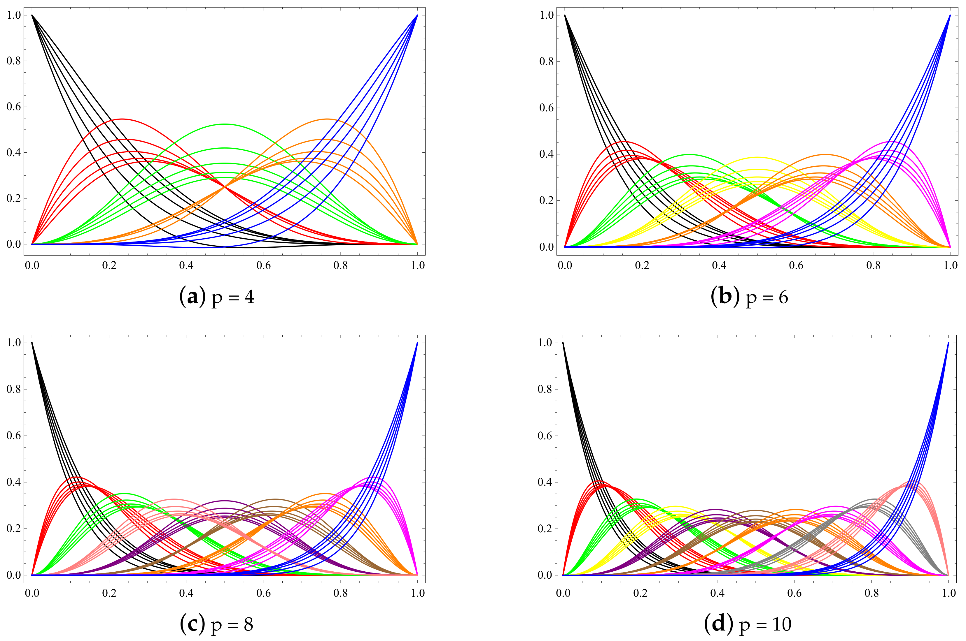
For integer p $(p\ge 3),$ the generalized hybrid trigonometric (GHT, for short) Bernstein basis functions [16] can be recursively written as follows

$${\mathfrak{F}}_{k,p}\left(\psi \right)=\psi {\mathfrak{F}}_{k-1,p-1}\left(\psi \right)+(1-\psi ){\mathfrak{F}}_{k,p-1}\left(\psi \right),\psi \in [0,1]$$

(2)

In addition, function ${\mathfrak{F}}_{k,p}\left(\psi \right)$ can be defined for integers $k>-1$ and $k\le p$. Figure 1 depicts some plots of GHT-Bernstein basis functions with different shape control parameters.

Theorem 1.

The p degree GHT-Bernstein basis function possesses some remarkable characteristics such as partition of unity, symmetry, non negativity, corner point interpolation property, and linear independence.

Proof. 

The proof of the properties is provided in [16]. □

3. GHT-Bézier Curves with Geometric Properties

Definition 2.

The p degree GHT-Bézier curves having shape control parameters $\xi ,\lambda ,{\xi }_3\in [-1,1],$, can be defined by GHT-Bernstein basis ${\mathfrak{F}}_{k,p}\left(\psi \right)$ and control points $\breve{g_k}$ as follows,

$${\Pi }_{p,\psi }:\varsigma (\psi ;\xi ,\lambda ,{\xi }_3)=\sum _{k=0}^p\breve{g_k}{\mathfrak{F}}_{k,p}\left(\psi \right),\psi \in [0,1].$$

(3)

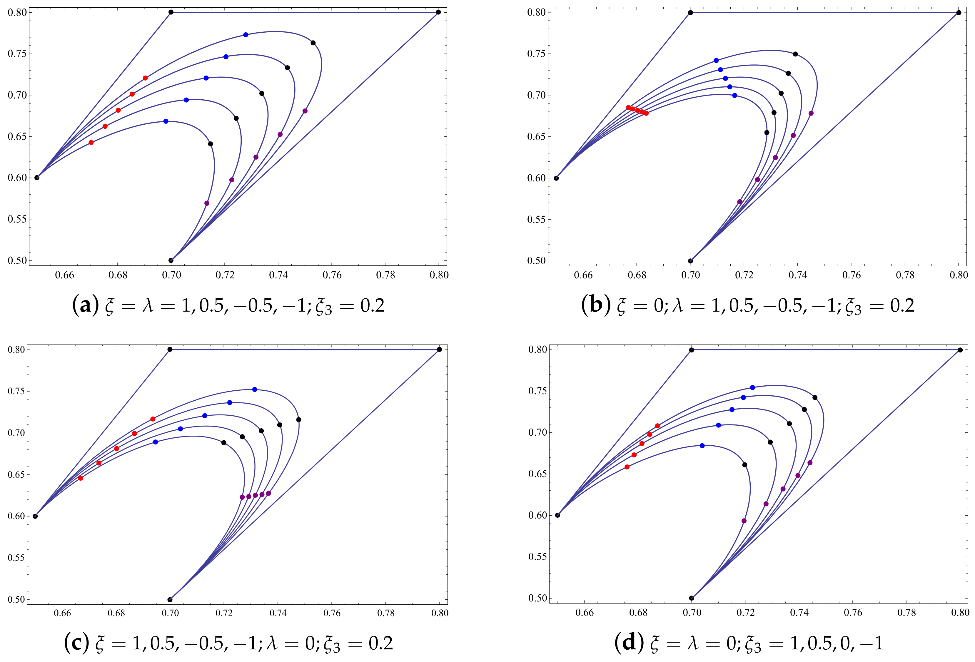
Figure 2 depicts some plots of GHT-Bézier curves with the shape control parameters taking different values.

Remark 1.

By having the multiple values of shape control parameters, the behavior of fixed points on GHT-Bézier curves are also affected as curves change.

In Figure 2, when the shape parameters $\xi =\lambda$ varies simultaneously while ${\xi }_3$ is fixed then curves inside the control polygon expand and the influence of these curves is at the center of the control polygon. These curves have the same behavior when the $\xi =\lambda =0$ and ${\xi }_3$ varies. When $\xi$ and ${\xi }_3$ fixed and $\lambda$ varies, then the influence of curves is on the right-hand side, while when $\lambda$ and ${\xi }_3$ fixed and $\xi$ varies, then influence of curves is on the left-hand side.

Theorem 2.

The GHT-Bézier curve has the following remarkable characteristics: shape adjustability, symmetry, convex hull property, geometric invariance, and endpoint properties.

Proof. 

The result can be deduced by using Definition 2 as in [16]. □

4. Composition of GHT-Bézier Developable Surfaces

4.1. Dual Representation of One-Parameter Family of Planes

The concept of dual representation is very helpful when we are dealing with GHT-Bézier developable surfaces. The single parameter family of control points, which are dual to a one-parameter family of planes $\left\{{\prod }_{\psi }\right\},$ can be obtained when we consider control points ${\breve{g}}_k$ as control planes. Thus in mathematical form we have

$$\left\{{\Pi }_{\psi }\right\}:\varsigma (\psi ;\xi ,\lambda ,{\xi }_3)=\sum _{k=0}^p\breve{g_k}{\mathfrak{F}}_{k,p}\left(\psi \right),\psi \in [0,1].$$

(4)

where the control planes and shape control parameters of the corresponding family of planes $\left\{{\Pi }_{\psi }\right\}$ are $\breve{g_k},(k=0,1,2,\cdots ,p)$ and $\xi ,\lambda ,{\xi }_3$, respectively. The coordinates of control planes are $\breve{g_k}=(s_k,t_k,u_k,v_k)$ with $(k=0,\cdots ,3).$ As stated duality of the vector form of one parameter family of planes is given as follows:

$$\begin{array}{ccc}\hfill \left\{{\Pi }_{\psi }\right\}:\varsigma (\psi ;\xi ,\lambda ,{\xi }_3)& =& \sum _{k=0}^n\breve{g_k}{\mathfrak{F}}_{k,p}\left(\psi \right)\hfill \\ & =& \sum _{k=0}^p(s_k,t_k,u_k,v_k){\mathfrak{F}}_{k,p}\left(\psi \right)\hfill \\ & =& \{{\wp }_0\left(\psi \right),{\wp }_1\left(\psi \right),{\wp }_2\left(\psi \right),{\wp }_3\left(\psi \right)\},\hfill \end{array}$$

where

$$\left\{\begin{array}{c}{\wp }_0\left(\psi \right)={\sum }_{k=0}^p{s}_k{\mathfrak{F}}_{k,p}\left(\psi \right)\hfill \\ {\wp }_1\left(\psi \right)={\sum }_{k=0}^p{t}_k{\mathfrak{F}}_{k,p}\left(\psi \right)\hfill \\ {\wp }_2\left(\psi \right)={\sum }_{k=0}^p{u}_k{\mathfrak{F}}_{k,p}\left(\psi \right)\hfill \\ {\wp }_3\left(\psi \right)={\sum }_{k=0}^p{v}_k{\mathfrak{F}}_{k,p}\left(\psi \right).\hfill \end{array}\right.$$

Briefly, we can write it as follows:

$$\begin{array}{c}\hfill \left\{{\Pi }_{\psi }\right\}:\varsigma (\psi ;\xi ,\lambda ,{\xi }_3)=\{{\wp }_0\left(\psi \right),{\wp }_1\left(\psi \right),{\wp }_2\left(\psi \right),{\wp }_3\left(\psi \right)\}.\end{array}$$

(5)

4.2. Enveloping Developable GHT-Bézier Surfaces

From the characteristics and basic definition of developable surfaces, we get that an enveloping developable surface is actually an envelope of a one-parameter family of planes $\left\{{\Pi }_{\psi }\right\},$ which can be written in linear equation as follows,

$$\begin{array}{c}\hfill ⅁\left(\psi \right)·X={\wp }_3\left(\psi \right),\end{array}$$

(6)

where $⅁\left(\psi \right)=({\wp }_0\left(\psi \right),{\wp }_1\left(\psi \right),{\wp }_2\left(\psi \right))$ and $X=(x,y,z).$ By differentiating Equation (6), we attain

$$\begin{array}{c}\hfill {⅁}^{{}^{\prime }}\left(\psi \right)·X={\wp }_3^{{}^{\prime }}\left(\psi \right),\end{array}$$

(7)

where ${⅁}^{{}^{\prime }}\left(\psi \right)=({\wp }_0^{{}^{\prime }}\left(\psi \right),{\wp }_1^{{}^{\prime }}\left(\psi \right),{\wp }_2^{{}^{\prime }}\left(\psi \right)).$ The intersecting lines of two planes defined in Equations (6) and (7) certainly lies on developable surfaces, known as the generator of developable surfaces w.r.t $\psi$.

The intersecting lines can be expressed as $\alpha \left(\psi \right),$

$$\alpha (\psi ;\xi ,\lambda ,{\xi }_3)=({ð}_1\left(\psi \right),{ð}_2\left(\psi \right)),$$

where

$$\begin{array}{ccc}\hfill {ð}_1\left(\psi \right)& =& ⅁\left(\psi \right)\times {⅁}^{{}^{\prime }}\left(\psi \right)\hfill \\ & =& \{{\wp }_1\left(\psi \right){\wp }_2^{{}^{\prime }}\left(\psi \right)-{\wp }_2\left(\psi \right){\wp }_1^{{}^{\prime }}\left(\psi \right),{\wp }_2\left(\psi \right){\wp }_0^{{}^{\prime }}\left(\psi \right)-{\wp }_0\left(\psi \right){\wp }_2^{{}^{\prime }}\left(\psi \right),{\wp }_0\left(\psi \right){\wp }_1^{{}^{\prime }}\left(\psi \right)-{\wp }_1\left(\psi \right){\wp }_0^{{}^{\prime }}\left(\psi \right)\},\hfill \end{array}$$

and

$${ð}_2\left(\psi \right)={\wp }_3^{{}^{\prime }}\left(\psi \right)⅁\left(\psi \right)-{\wp }_3\left(\psi \right){⅁}^{{}^{\prime }}\left(\psi \right).$$

${ð}_1\left(\psi \right)$ is the direction vector of the intersecting line $\alpha \left(\psi \right)$ and ${ð}_2\left(\psi \right)$ is the vector along $\alpha \left(\psi \right).$

Suppose that $V\left(\psi \right)$ is the closest point on $\alpha \left(\psi \right)$ to origin. So, the point $V\left(\psi \right)$ can be obtained in the form of the following coordinates,

$$V\left(\psi \right)=\frac{{ð}_1\left(\psi \right)\times {ð}_2\left(\psi \right)}{{ð}_1\left(\psi \right)·{ð}_1\left(\psi \right)}$$

(8)

$$\begin{array}{cc}\hfill & V\left(\psi \right)=\{[{\wp }_2\left(\psi \right){\wp }_0^{{}^{\prime }}\left(\psi \right)-{\wp }_0\left(\psi \right){\wp }_2^{{}^{\prime }}\left(\psi \right)][{\wp }_2\left(\psi \right){\wp }_3^{{}^{\prime }}\left(\psi \right)-{\wp }_3\left(\psi \right){\wp }_2^{{}^{\prime }}\left(\psi \right)]-[{\wp }_0\left(\psi \right){\wp }_1^{{}^{\prime }}\left(\psi \right)-{\wp }_1\left(\psi \right){\wp }_0^{{}^{\prime }}\left(\psi \right)]\\ & [{\wp }_1\left(\psi \right){\wp }_3^{{}^{\prime }}\left(\psi \right)-{\wp }_3\left(\psi \right){\wp }_1^{{}^{\prime }}\left(\psi \right)],[{\wp }_0\left(\psi \right){\wp }_1^{{}^{\prime }}\left(\psi \right)-{\wp }_1\left(\psi \right){\wp }_0^{{}^{\prime }}\left(\psi \right)][{\wp }_0\left(\psi \right){\wp }_3^{{}^{\prime }}\left(\psi \right)-{\wp }_3\left(\psi \right){\wp }_0^{{}^{\prime }}\left(\psi \right)]-\\ & [{\wp }_1\left(\psi \right){\wp }_2^{{}^{\prime }}\left(\psi \right)-{\wp }_2\left(\psi \right){\wp }_1^{{}^{\prime }}\left(\psi \right)][{\wp }_2\left(\psi \right){\wp }_3^{{}^{\prime }}\left(\psi \right)-{\wp }_3\left(\psi \right){\wp }_2^{{}^{\prime }}\left(\psi \right)],[{\wp }_1\left(\psi \right){\wp }_2^{{}^{\prime }}\left(\psi \right)-{\wp }_2\left(\psi \right){\wp }_1^{{}^{\prime }}\left(\psi \right)]\\ & [{\wp }_1\left(\psi \right){\wp }_3^{{}^{\prime }}\left(\psi \right)-{\wp }_3\left(\psi \right){\wp }_1^{{}^{\prime }}\left(\psi \right)]-[{\wp }_2\left(\psi \right){\wp }_0^{{}^{\prime }}\left(\psi \right)-{\wp }_0\left(\psi \right){\wp }_2^{{}^{\prime }}\left(\psi \right)][{\wp }_0\left(\psi \right){\wp }_3^{{}^{\prime }}\left(\psi \right)-{\wp }_3\left(\psi \right){\wp }_0^{{}^{\prime }}\left(\psi \right)]\}/\\ & {[{\wp }_1\left(\psi \right){\wp }_2^{{}^{\prime }}\left(\psi \right)-{\wp }_2\left(\psi \right){\wp }_1^{{}^{\prime }}\left(\psi \right)]}^2{[{\wp }_2\left(\psi \right){\wp }_0^{{}^{\prime }}\left(\psi \right)-{\wp }_0\left(\psi \right){\wp }_2^{{}^{\prime }}\left(\psi \right)]}^2+{[{\wp }_0\left(\psi \right){\wp }_1^{{}^{\prime }}\left(\psi \right)-{\wp }_1\left(\psi \right){\wp }_0^{{}^{\prime }}\left(\psi \right)]}^2.\end{array}$$

So, the intersecting line $\alpha (\psi ;\xi ,\lambda ,{\xi }_3)$ in parametric form can be written as follows,

$$\alpha (\psi ,t;\xi ,\lambda ,{\xi }_3)=t{ð}_1\left(\psi \right)+V\left(\psi \right),wheret\in (-\infty ,+\infty ),\psi \in [0,1],$$

(9)

where $\xi ,\lambda ,{\xi }_3\in [0,1]$ are the shape control parameters. For distinct values of shape control parameters, a class of GHT-Bézier enveloping developable surfaces with one-parameter family of planes $\left\{{\Pi }_{\psi }\right\}$ can be constructed by using Equation (9).

4.3. Spine Curve Developable GHT-Bézier Surfaces

Another approach for the construction of developable surfaces is spine curve developable GHT-Bézier surface. In a single parameter family of planes $\left\{{\Pi }_{\psi }\right\},$ three successive planes defined in Equations (6) and (7) and the plane produced as follows,

$$\begin{array}{c}\hfill {⅁}^{{}^{″}}\left(\psi \right)·X={\wp }_3^{{}^{″}}\left(\psi \right),\end{array}$$

(10)

where ${⅁}^{{}^{″}}\left(\psi \right)=({\wp }_0^{{}^{″}}\left(\psi \right),{\wp }_1^{{}^{″}}\left(\psi \right),{\wp }_2^{{}^{″}}\left(\psi \right)),$$X=(x,y,z)$ and double prime denotes the second derivative), intersects at a point called characteristic point. So, the characteristic/intersecting point can be determined by the following set of simultaneous equations,

$$\begin{array}{c}\hfill \left\{\begin{array}{c}⅁\left(\psi \right)·X={\wp }_3\left(\psi \right),\hfill \\ {⅁}^{{}^{\prime }}\left(\psi \right)·X={\wp }_3^{{}^{\prime }}\left(\psi \right),\hfill \\ {⅁}^{{}^{″}}\left(\psi \right)·X={\wp }_3^{{}^{″}}\left(\psi \right),\hfill \end{array}\right.\end{array}$$

(11)

and by solving above equations, we get the following expression

$$\begin{array}{c}\hfill \aleph \left(\psi \right)=\frac{{\wp }_3^{{}^{″}}\left(\psi \right)(⅁\left(\psi \right)\times {⅁}^{{}^{\prime }}\left(\psi \right))+{\wp }_3\left(x\right)({⅁}^{{}^{\prime }}\left(\psi \right)\times {⅁}^{{}^{\prime \prime }}\left(\psi \right))+{\wp }_3^{{}^{\prime }}\left(\psi \right)({⅁}^{{}^{\prime \prime }}\left(\psi \right)\times ⅁\left(\psi \right))}{({⅁}^{{}^{\prime }}\left(\psi \right)\times {⅁}^{{}^{″}}\left(\psi \right))·⅁\left(\psi \right)}.\end{array}$$

(12)

Hence, the coordinates of characteristic points $\aleph \left(\psi \right)$ are,

$$x=\frac{1}{\zeta \left(\psi \right)}\left|\begin{array}{ccc}{\wp }_3\left(\psi \right)& {\wp }_1\left(\psi \right)& {\wp }_2\left(\psi \right)\\ {\wp }_3^{{}^{\prime }}\left(\psi \right)& {\wp }_1^{{}^{\prime }}\left(\psi \right)& {\wp }_2^{{}^{\prime }}\left(\psi \right)\\ {\wp }_3^{{}^{″}}\left(\psi \right)& {\wp }_1^{{}^{″}}\left(\psi \right)& {\wp }_2^{{}^{″}}\left(\psi \right)\end{array}\right|,y=\frac{1}{\zeta \left(\psi \right)}\left|\begin{array}{ccc}{\wp }_0\left(\psi \right)& {\wp }_3\left(\psi \right)& {\wp }_2\left(\psi \right)\\ {\wp }_0^{{}^{\prime }}\left(\psi \right)& {\wp }_3^{{}^{\prime }}\left(\psi \right)& {\wp }_2^{{}^{\prime }}\left(\psi \right)\\ {\wp }_0^{{}^{″}}\left(\psi \right)& {\wp }_3^{{}^{″}}\left(\psi \right)& {\wp }_2^{{}^{″}}\left(\psi \right)\end{array}\right|,z=\frac{1}{\zeta \left(\psi \right)}\left|\begin{array}{ccc}{\wp }_0\left(\psi \right)& {\wp }_1\left(\psi \right)& {\wp }_3\left(\psi \right)\\ {\wp }_0^{{}^{\prime }}\left(\psi \right)& {\wp }_1^{{}^{\prime }}\left(\psi \right)& {\wp }_3^{{}^{\prime }}\left(\psi \right)\\ {\wp }_0^{{}^{″}}\left(\psi \right)& {\wp }_1^{{}^{″}}\left(\psi \right)& {\wp }_3^{{}^{″}}\left(\psi \right)\end{array}\right|,$$

and

$$\zeta \left(\psi \right)=\left|\begin{array}{ccc}{\wp }_0\left(\psi \right)& {\wp }_1\left(\psi \right)& {\wp }_2\left(\psi \right)\\ {\wp }_0^{{}^{\prime }}\left(\psi \right)& {\wp }_1^{{}^{\prime }}\left(\psi \right)& {\wp }_2^{{}^{\prime }}\left(\psi \right)\\ {\wp }_0^{{}^{″}}\left(\psi \right)& {\wp }_1^{{}^{″}}\left(\psi \right)& {\wp }_2^{{}^{″}}\left(\psi \right)\end{array}\right|.$$

So, spine curve developable GHT-Bézier surface can be written as follows,

$$S(\psi ,k;\xi ,\lambda ,{\xi }_3)=\aleph \left(\psi \right)+k{\aleph }^{{}^{\prime }}\left(\psi \right),\psi \in [0,1],k\in (-\infty ,\infty )$$

(13)

It is noted from Equations (9) and (13) that GHT-Bézier developable surfaces are dissimilar to the tensor product GHT-Bézier surfaces. However, these developable surfaces can also be acquired by using GHT-Bernstein basis function as like GHT-Bézier tensor product surface. Therefore, the developable GHT-Bézier surface have similar properties as GHT-Bézier curve.

4.4. Developable Surface Interpolating Geodesic GHT-Bézier Curve

In geometry, the shortest curved path between any two points on the surface is known as a geodesic. The acceleration of the geodesic curve is always zero at every point.

The developable surface interpolation geodesic GHT-Bézier curve and by having multiple values of shape control parameters a family of geodesic interpolation developable surfaces can be constructed in this section.

Theorem 3.

A curve on a surface $⅁(\psi ,k;\xi ,\lambda ,{\xi }_3)$ can only be the geodesic when principle normal $\rho \left(\psi \right)$ is parallel to the normal $N(k_0,\psi )$ at each point of the curve.

Proof. 

Suppose that $⅁(k,\psi ;\xi ,\lambda ,{\xi }_3)$ is a surface, $\varsigma \left(\psi \right)$ be a curve on the surface and $\omega$ is any point on the curve. $\rho \left(\psi \right)$ is the principle normal and $N(k_0,\psi )$ is the normal vector at point $\omega$, respectively. $\kappa$ is the geodesic curvature and $\beta$ is the angle between principle normal and normal vector. So, using geodesic curvature we have

$$\kappa =\pm \ell sin\left(\beta \right)=0.$$

Since $\ell \ne 0,$ so $\beta =0$ or $\beta =\pi$ and principle normal will be parallel to normal vector. □

Theorem 4.

When a GHT-Bézier curve with shape parameters $\xi ,\lambda ,{\xi }_3$ is given, a developable surface that is geodesic to the GHT-Bézier developable surface must exist through it.

Proof. 

Suppose that $\varsigma \left(\psi \right)$ is a cubic GHT-Bézier curve, then its ruled surface is given as,

$$⅁(\psi ,k;\xi ,\lambda ,{\xi }_3)=\varsigma (\psi ;\xi ,\lambda ,{\xi }_3)+k{\varsigma }_1(\psi ;\xi ,\lambda ,{\xi }_3),$$

(14)

while as we described in Theorem 3, the curve $\varsigma \left(\psi \right)$ is geodesic on the surface $⅁(\psi ,k;\xi ,\lambda ,{\xi }_3).$ So, we have

$$⅁(\psi ,0;\xi ,\lambda ,{\xi }_3)=\varsigma (\psi ;\xi ,\lambda ,{\xi }_3),\rho (\psi ;\xi ,\lambda ,{\xi }_3)\left|\right|N(\psi ,0;\xi ,\lambda ,{\xi }_3),$$

(15)

where $\rho (\psi ;\xi ,\lambda ,{\xi }_3)$ and $N(\psi ,0;\xi ,\lambda ,{\xi }_3)$ are principle normal and normal vector of the curve respectively. For simplicity,

$$\begin{array}{ccc}\hfill N(\psi ,0)& =& {⅁}_{\psi }\times {⅁}_k\hfill \\ & =& [{\varsigma }^{\prime }\left(\psi \right)+k\left({\varsigma }_1^{\prime }\left(\psi \right)\right]\times {\varsigma }_1\left(\psi \right)\hfill \\ & =& {\varsigma }^{\prime }\left(\psi \right)\times {\varsigma }_1^{\prime }\left(\psi \right),\hfill \end{array}$$

and

$$\rho \left(\psi \right)=\frac{[{\varsigma }^{\prime }\left(\psi \right).{\varsigma }^{\prime }\left(\psi \right)]·{\varsigma }^{″}\left(\psi \right)-[{\varsigma }^{\prime }\left(\psi \right)·{\varsigma }^{″}\left(\psi \right)].{\varsigma }^{\prime }\left(\psi \right)}{|{\varsigma }^{\prime }\left(\psi \right)\left|\right|{\varsigma }^{\prime }\left(\psi \right)\times {\varsigma }^{″}\left(\psi \right)|}$$

where $\rho \left(\psi \right)$ is parallel to $N(\psi ,0)$ and ${\varsigma }^{\prime }\left(\psi \right)$ is perpendicular to $N(\psi ,0),$ while the vector ${\varsigma }_1\left(\psi \right)$ must be in the plane spanned by ${\varsigma }^{\prime }\left(\psi \right)$ and ${\varsigma }^{\prime }\left(\psi \right)\times {\varsigma }^{″}\left(\psi \right).$

Consider

$${\varsigma }_1\left(\psi \right)={\nu }_1{\varsigma }^{\prime }\left(\psi \right)+{\nu }_2({\varsigma }^{\prime }\left(\psi \right)\times {\varsigma }^{″}\left(\psi \right)).$$

So, according to the condition of developable surface, we

$$\begin{array}{ccc}\hfill [{\varsigma }^{\prime }\left(\psi \right),{\nu }_1{\varsigma }^{\prime }\left(\psi \right)+{\nu }_2({\varsigma }^{\prime }\left(\psi \right)\times {\varsigma }^{″}\left(\psi \right)),({\nu }_1{\varsigma }^{\prime }\left(\psi \right)+{\nu }_2({\varsigma }^{\prime }\left(\psi \right)\times {\varsigma }^{″}\left(\psi \right)))]& =& 0\hfill \\ \hfill \iff [{\varsigma }^{\prime }\left(\psi \right),{\nu }_1{\varsigma }^{\prime }\left(\psi \right)+{\nu }_2({\varsigma }^{\prime }\left(\psi \right)\times {\varsigma }^{″}\left(\psi \right)),{\nu }_1^{\prime }{\varsigma }^{\prime }\left(\psi \right)+{\nu }_1{\varsigma }^{″}\left(\psi \right)+{\nu }_2^{\prime }{\varsigma }^{\prime }\left(\psi \right)\times {\varsigma }^{″}\left(\psi \right)+{\nu }_2{\varsigma }^{\prime }\left(\psi \right)\times {\varsigma }^{‴}\left(\psi \right)]& =& 0\hfill \\ \hfill \iff [{\varsigma }^{\prime }\left(\psi \right),{\nu }_2({\varsigma }^{\prime }\left(\psi \right)\times {\varsigma }^{″}\left(\psi \right)),{\nu }_1{\varsigma }^{″}\left(\psi \right)+{\nu }_2^{\prime }{\varsigma }^{\prime }\left(\psi \right)\times {\varsigma }^{″}\left(\psi \right)+{\nu }_2{\varsigma }^{\prime }\left(\psi \right)\times {\varsigma }^{‴}\left(\psi \right)]& =& 0\hfill \\ \hfill \iff [({\varsigma }^{\prime }\left(\psi \right)\times {\varsigma }^{″}\left(\psi \right))\times {\varsigma }^{\prime }\left(\psi \right)]·({\nu }_1{\varsigma }^{″}\left(\psi \right)+{\nu }_2{\varsigma }^{\prime }\left(\psi \right)\times {\varsigma }^{″\prime }\left(\psi \right))& =& 0\hfill \\ \hfill \iff \left[\right|{\varsigma }^{\prime }{\left(\psi \right)|}^2|{\varsigma }^{″}{\left(\psi \right)|}^2-|{\varsigma }^{\prime }\left(\psi \right)·{\varsigma }^{″}{\left(\psi \right)|}^2]{\nu }_1={\left|{\varsigma }^{\prime }\left(\psi \right)\right|}^2({\varsigma }^{\prime }\left(\psi \right),{\varsigma }^{″}\left(\psi \right),{\varsigma }^{″\prime }\left(\psi \right)){\nu }_2.\end{array}$$

Which implies,

$$\begin{array}{c}⅁(\psi ,k;\xi ,\lambda ,{\xi }_3)=\varsigma (\psi ;\xi ,\lambda ,{\xi }_3)+k({\nu }_1{\varsigma }^{\prime }(\psi ;\xi ,\lambda ,{\xi }_3)+{\nu }_2({\varsigma }^{\prime }(\psi ;\xi ,\lambda ,{\xi }_3)\times {\varsigma }^{″}(\psi ;\xi ,\lambda ,{\xi }_3))),\hfill \\ & \hfill \psi \in [0,1],k\in (-\infty ,+\infty ).\end{array}$$

(16)

Which shows that the curves $\varsigma \left(\psi \right)$ and ${\varsigma }^{\prime }\left(\psi \right)$ are geodesics on developable GHT-Bézier surface. □

4.5. Developable GHT-Bézier Canal Surface

Canal surfaces have wide applications in CAGD, such as the construction of blending surfaces, shape reconstruction, transition surfaces between pipes, robotic path planning, etc.

A canal surface is a surface formed as the envelope of a family of spheres whose center lies at a space curve framed by {T, N, B} with radius $r\left(\psi \right)$ same as the radius of the sphere. Suppose that the center curve of a canal surface is a GHT-Bézier curve, then the general canal surface can be parameterized by the formula

$$x(\psi ,s)=\varsigma (\psi ;\xi ,\lambda ,{\xi }_3)+\sigma \left(\psi \right)T\left(\psi \right)+\mu (\psi ,s)N\left(\psi \right)+\omega (\psi ,s)B\left(\psi \right)$$

(17)

where $\sigma ,\mu$, and $\omega$ are differential functions of $\psi$ and $s.$ If the canal surface is formed by the movement of pseudohyperbolic sphere along a space-like curve, then we get

$$\left\{\begin{array}{c}\sigma \left(\psi \right)=r\left(\psi \right)r^{\prime }\left(\psi \right)\hfill \\ \mu (\psi ,s)=r\left(\psi \right)\sqrt{1+r^{\prime 2}\left(\psi \right)}sinh\left(s\right)\hfill \\ \omega (\psi ,s)=r\left(\psi \right)\sqrt{1+r^{\prime 2}\left(\psi \right)}cosh\left(s\right).\hfill \end{array}\right.$$

(18)

Proposition 1.

The quantities of first and second fundamental form of canal surface satisfy

$$L=\frac{E-\xi }{-r},M=\frac{F}{-r^{\prime }},N\frac{G}{-r},$$

and

$$EG-F^2=r^2{\xi }^2,LN-M^2=r\xi {\xi }^{*},$$

where

$$\xi =rr"-r\kappa sinh\left(\varphi \right)cos\left(s\right)+sin{h}^2\left(\varphi \right)=r{\xi }^{*}+sinh\left(\varphi \right),{\xi }^{*}=r"-\kappa sinh\left(\varphi \right)cos\left(s\right).$$

Due to regularity, $\xi \ne 0$ everywhere by the first and second fundamental form of canal surface.

So, the Gaussian curvature κ and Mean curvature H of the canal surface is given by,

$$\kappa =-\frac{LN-M^2}{EG-F^2}=-\frac{{\xi }^{*}}{r\xi }$$

(19)

$$H=-\frac{EN-2FM+GL}{2(GE-F^2)}=\frac{2\xi -{sinh}^2\left(\varphi \right)}{2r\xi }$$

(20)

Theorem 5.

A canal surface is developable if it is a circular cone.

Proof. 

A canal surface is developable if $\kappa =0.$ By Equation (19), we have ${\xi }^{*}=0.$ Then we get

$$r"\left(\psi \right)-\kappa sinh\left(\varphi \right)cos\left(s\right)=0.$$

It follows $r^{"}\left(\psi \right)=0$ and $\kappa =0,$ (if $sinh\left(\varphi \right)=0,$ by first and second fundamental form as given in Proposition 1, the canal surface degenerate). Then

$$r\left(\psi \right)=c_1\psi +c_2,$$

where $c_1$ and $c_2$ are constants and $|c_1|>1.$ If $|c_1\le 1|,$ by Equation (17) it is a contradiction. Therefore, the canal surface is a circular cone. The converse of this theorem is obvious. □

5. Analysis Properties of Developable GHT-Bézier Surfaces

According to the duality principle, the relationship between developable GHT-Bézier surfaces and control planes is similar as between its dual curve and control points. Based on single parameter family of planes ${\Pi }_{\psi },$ the Equation (22) can be obtained by taking first and second derivative of the Equation (21).

$$\varsigma (\psi ;\xi ,\lambda ,{\xi }_3)=\sum _{i=0}^3\breve{g_k}{\mathfrak{F}}_{k,3}\left(\psi \right),\psi \in [0,1]$$

(21)

we have,

$$\left\{\begin{array}{c}{\varsigma }^{\prime }(\psi ;\xi ,\lambda ,{\xi }_3)=\breve{g_0}{\mathfrak{F}}_{k,3}^{\prime }\left(\psi \right)+\breve{g_1}{\mathfrak{F}}_{k,3}^{\prime }\left(\psi \right)+\breve{g_2}{\mathfrak{F}}_{k,3}^{\prime }\left(\psi \right)+\breve{g_3}{\mathfrak{F}}_{k,3}^{\prime }\left(\psi \right),\hfill \\ {\varsigma }^{″}(\psi ;\xi ,\lambda ,{\xi }_3)=\breve{g_0}{\mathfrak{F}}_{k,3}^{″}\left(\psi \right)+\breve{g_1}{\mathfrak{F}}_{k,3}^{″}\left(\psi \right)+\breve{g_2}{\mathfrak{F}}_{k,3}^{″}\left(\psi \right)+\breve{g_3}{\mathfrak{F}}_{k,3}^{″}\left(\psi \right).\hfill \end{array}\right.$$

(22)

So, the planes corresponding to $\psi =0$ and $\psi =1$ meet the following axioms,

$$\begin{array}{ccc}\hfill \varsigma \left(0\right)& =& {\breve{g}}_0\hfill \\ \hfill \varsigma \left(1\right)& =& {\breve{g}}_p\hfill \\ \hfill {\varsigma }^{\prime }\left(0\right)& =& ((p-2)+\frac{\pi }{2}(1+\xi )-{\xi }_3)({\breve{g}}_1-{\breve{g}}_0)\hfill \\ \hfill {\varsigma }^{\prime }\left(1\right)& =& ((p-2)+\frac{\pi }{2}(1+\lambda )-{\xi }_3)({\breve{g}}_p-{\breve{g}}_{p-1})\hfill \\ \hfill {\varsigma }^{″}\left(0\right)& =& \frac{1}{4}\{\left[2({\pi }^2\xi -2\pi (1+{\xi }_1)({\xi }_3-2(p-2)))\right]{\breve{g}}_0-2[{\pi }^2{\xi }_1-2\pi (1+\xi )({\xi }_3-2(p-2))+2(2(p-2)\hfill \\ & & (p-3)+({\xi }_3-4(p-2)){\xi }_3\left)\right]{\breve{g}}_1+e^{{\xi }_3}{\pi }^2(-1+\lambda )({\breve{g}}_1-{\breve{g}}_2)+4(p-2)[(p-3)+\pi +\pi \xi -2{\xi }_3]\}{\breve{g}}_2,\hfill \\ \hfill {\varsigma }^{″}\left(1\right)& =& \frac{1}{4}\{-e^{{\xi }_3}{\pi }^2(\xi -1)({\breve{g}}_{p-2}-{\breve{g}}_{p-1})+2[2(p-2)(p-3+\pi +\pi \lambda -2{\xi }_3){\breve{g}}_{p-2}-({\pi }^2\lambda -2\pi (1+\lambda )\hfill \\ & & ({\xi }_3-2(p-2))+2(2(p-2)(p-3)+({\xi }_3-4(p-2)){\xi }_3)){\breve{g}}_{n-1}+({\pi }^2{\xi }_2-2\pi (1+\lambda )({\xi }_3-(p-2))\hfill \\ & & +2((p-2)(p-3)+({\xi }_3-2(p-2)){\xi }_3)){\breve{g}}_p\left]\right\}.\hfill \end{array}$$

The intersection of two planes obtained as $\varsigma \left(0\right)$ and ${\varsigma }^{\prime }\left(0\right)$ is called the starting generator while the intersection of planes obtained as $\varsigma \left(1\right)$ and ${\varsigma }^{\prime }\left(1\right)$ is called the ending generator of developable GHT-Bézier surface. The first and last planes defined in the above equation are tangential along their generators at $\psi =0$ and $\psi =1$ to the developable surface. The control planes ${\breve{g}}_0,{\breve{g}}_1,{\breve{g}}_2$ are the characteristic points on starting generator while control planes ${\breve{g}}_1,{\breve{g}}_2,{\breve{g}}_3$ are characteristic points on the ending generator.

6. Continuity Conditions of Developable GHT-Bézier Surfaces

In the CAD/CAM field, the developable GHT-Bézier surfaces are widely applicable for various designs to attain complex products by adjoining two developable surfaces. In this section, the continuity conditions are derived between two adjacent GHT-Bézier developable surfaces i.e., $G^1$ continuity and Farin-Boehm and Beta $\left(G^2\right)$ continuity as in [2,3,4,5,6,7,8,9]. Here, one more contribution made for the developable GHT-Bézier surfaces is $G^3$ continuity in $4D$ projective space.

Consider any two GHT-Bézier developable surfaces with three different shape control parameters $\xi ,\lambda ,{\xi }_3,\breve{\xi },\breve{\lambda },\breve{{\xi }_3}$ spliced together, whose expression can be defined as follows:

$$\left\{\begin{array}{c}\left\{{\Pi }_{\psi ,1}\right\}:{\varsigma }_1(\psi ;\xi ,\lambda ,{\xi }_3)={\sum }_{k=0}^p\breve{g_k}{\mathfrak{F}}_{k,p}\left(\psi \right),\hfill \\ \left\{{\Pi }_{\psi ,2}\right\}:{\varsigma }_2(\psi ;\breve{\xi },\breve{\lambda },\breve{{\xi }_3})={\sum }_{j=0}^m\breve{z_j}{\mathfrak{F}}_{j,m}\left(\psi \right),\hfill \end{array}\right.$$

(23)

where $\breve{g_k}$ and $\breve{z_j}$ are the control planes for one parameter family of planes $\left\{{\Pi }_{\psi ,1}\right\}$ and $\left\{{\Pi }_{\psi ,2}\right\}$, respectively, and ${\mathfrak{F}}_{k,p}\left(\psi \right)$ and ${\mathfrak{F}}_{j,m}\left(\psi \right)$ are respective GHT-Bernstein basis functions.

6.1. Axioms of $G^1$ Continuity between Developable GHT-Bézier Surfaces

Theorem 6.

The axioms between two GHT-Bézier developable surfaces ${\varsigma }_1(\psi ;\xi ,\lambda ,{\xi }_3)$ and ${\varsigma }_2(\psi ;\breve{\xi },\breve{\lambda },\breve{{\xi }_3})$ at the joints are given as:

$$\begin{array}{ccc}\hfill {\breve{z}}_0& =& {\breve{g}}_p,\hfill \end{array}$$

(24)

$$\begin{array}{ccc}\hfill {\breve{z}}_1& =& {\breve{g}}_p-\frac{2((p-2)-{\xi }_3+\frac{\pi }{2}(1+\lambda ))}{2((p-2)-{\breve{\xi }}_3+\frac{\pi }{2}(1+\breve{\xi }))\gamma }({\breve{g}}_{p-1}-{\breve{g}}_p).\hfill \end{array}$$

(25)

Proof. 

To achieve $G^1$ continuity of developable GHT-Bézier surfaces ${\varsigma }_1(\psi ;\xi ,\lambda ,{\xi }_3)$ and ${\varsigma }_2(\psi ;\breve{\xi },\breve{\lambda },\breve{{\xi }_3}),$ it is necessary to achieve $G^0$ continuity first, which means

$${\varsigma }_1(1;\xi ,\lambda ,{\xi }_3)={\varsigma }_2(0;\breve{\xi },\breve{\lambda },\breve{{\xi }_3}).$$

So, by using analysis properties of developable GHT-Bézier surfaces we obtained

$${\breve{g}}_n={\breve{z}}_0.$$

For $G^1$ continuity conditions, the developable GHT-Bézier surfaces must have the same tangent plane at common points. Which means

$${\varsigma }_1^{\prime }(1;\xi ,\lambda ,{\xi }_3)=\gamma {\varsigma }_2^{\prime }(0;\breve{\xi },\breve{\lambda },\breve{{\xi }_3}),$$

where $\gamma$ is the positive scale factor and by having analysis properties of developable GHT-Bézier surfaces, we get

$${\breve{z}}_1={\breve{g}}_p-\frac{2((p-2)-{\xi }_3+\frac{\pi }{2}(1+\lambda ))}{2((p-2)-{\breve{\xi }}_3+\frac{\pi }{2}(1+\breve{\xi }))\gamma }({\breve{g}}_{p-1}-{\breve{g}}_p).$$

□

6.2. Axioms of Farin-Boehm $G^2$ Continuity between Developable GHT-Bézier Surfaces

Theorem 7.

The necessary and sufficient conditions for Farin-Boehm $G^2$ continuity between two adjacent developable GHT-Bézier surfaces ${\varsigma }_1(\psi ;\xi ,\lambda ,{\xi }_3)$ and ${\varsigma }_2(\psi ;\breve{\xi },\breve{\lambda },\breve{{\xi }_3}),$ at the joints are

$$\left\{\begin{array}{c}{\breve{z}}_0={\breve{g}}_p,\hfill \\ {\breve{z}}_1={\breve{g}}_p-\frac{2((p-2)-{\xi }_3+\frac{\pi }{2}(1+\lambda ))}{2((p-2)-{\breve{\xi }}_3+\frac{\pi }{2}(1+\breve{\xi }))}({\breve{g}}_{p-1}-{\breve{g}}_p),\hfill \\ {\breve{z}}_2=[\{-4(p-2)(p-3)+8(p-2){\xi }_3-4(p-2)(\lambda +1)\pi +e^{{\xi }_3}{\pi }^2(\xi -1)\}{\breve{g}}_{p-2}\hfill \\ -\{4\pi (1+\lambda )({\xi }_3-4(p-2))-4({\xi }_3({\xi }_3-4(p-2))+2(p-2)(p-3))+{\pi }^2(-2\lambda +e_3^{\xi }\hfill \\ (\xi -1)\left)\right\}{\breve{g}}_{p-1}+\{-4(p-2)\pi \lambda -2{\pi }^2\lambda +8(p-2){\xi }_3+4\pi {\xi }_3+4\pi \lambda {\xi }_3-4{\xi }_3^2-8(p-2){\breve{\xi }}_3\hfill \\ -4\pi {\breve{\xi }}_3+4{\breve{\xi }}_3^2+4(p-2)\pi \breve{\xi }+2{\pi }^2\breve{\xi }-4\pi {\breve{\xi }}_3\breve{\xi }\}{\breve{g}}_p+\frac{1}{a}]h\hfill \\ where\hfill \\ a=(2(p-2)+\pi -2{\breve{\xi }}_3+\pi \breve{\xi })[-4(2(p-2)(p-3)+({\breve{\xi }}_3-4(p-2)){\breve{\xi }}_3)+{\pi }^2(e^{{\breve{\xi }}_3}(\breve{\lambda }-1)\hfill \\ -2\breve{\xi })+4\pi ({\breve{\xi }}_3-2(p-2))(1+\breve{\xi })\left]\right(-(2(p-2)+\pi +\pi \lambda -2{\xi }_3){\breve{p}}_{p-1}+(-2(-2(p-2)+{\xi }_3\hfill \\ +{\breve{\xi }}_3)+\pi (2+\lambda +\breve{\xi })\left){\breve{g}}_p\right)\hfill \\ and\hfill \\ h=\frac{1}{(8(p-2){\breve{\xi }}_3-4(p-2)(p-3)-4(p-2)\pi (1+\breve{\xi })+{\pi }^2{e}^{{\breve{\xi }}_3}(\breve{\lambda }-1))}.\hfill \end{array}\right.$$

(26)

Proof. 

To reach Farin-Boehm $G^2$ continuity conditions between two developable GHT-Bézier surfaces ${\varsigma }_1(\psi ;\xi ,\lambda ,{\xi }_3)$ and ${\varsigma }_2(\psi ;\breve{\xi },\breve{\lambda },\breve{{\xi }_3}),$ they must need to fulfill $G^0$ and $G^1$ continuity first. i.e.,

$${\varsigma }_1(1;\xi ,\lambda ,{\xi }_3)={\varsigma }_2(0;\breve{\xi },\breve{\lambda },\breve{{\xi }_3}),$$

and

$${\varsigma }_1^{\prime }(1;\xi ,\lambda ,{\xi }_3)={\varsigma }_2^{\prime }(0;\breve{\xi },\breve{\lambda },\breve{{\xi }_3}).$$

Which means that these two surfaces must have same common point and common tangent plane. So, from analysis properties of developable GHT-Bézier surfaces we get

$$\begin{array}{ccc}\hfill {\breve{z}}_0& =& {\breve{g}}_p,\hfill \end{array}$$

(27)

$$\begin{array}{ccc}\hfill {\breve{z}}_1& =& {\breve{g}}_p-\frac{2((p-2)-{\xi }_3+\frac{\pi }{2}(1+\lambda ))}{2((p-2)-{\breve{\xi }}_3+\frac{\pi }{2}(1+\breve{\xi }))}({\breve{g}}_{p-1}-{\breve{g}}_p).\hfill \end{array}$$

(28)

Now, for Farin-Boehm $G^2$ continuity conditions we have the following condition

$${\varsigma }_1^{″}(1;\xi ,\lambda ,{\xi }_3)={\varsigma }_2^{″}(0;\breve{\xi },\breve{\lambda },\breve{{\xi }_3}),$$

and for end point properties of developable GHT-Bézier surfaces we obtained

$$\left\{\begin{array}{c}{\breve{z}}_2=[\{-4(p-2)(p-3)+8(p-2){\xi }_3-4(p-2)(\lambda +1)\pi +e^{{\xi }_3}{\pi }^2(\xi -1)\}{\breve{g}}_{p-2}\hfill \\ -\{4\pi (1+\lambda )({\xi }_3-4(p-2))-4({\xi }_3({\xi }_3-4(p-2))+2(p-2)(p-3))+{\pi }^2(-2\lambda +e_3^{\xi }\hfill \\ ({\xi }_1-1)\left)\right\}{\breve{g}}_{p-1}+\{-4(p-2)\pi \lambda -2{\pi }^2\lambda +8(p-2){\xi }_3+4\pi {\xi }_3+4\pi \lambda {\xi }_3-4{\xi }_3^2-8(p-2){\breve{\xi }}_3\hfill \\ -4\pi {\breve{\xi }}_3+4{\breve{\xi }}_3^2+4(p-2)\pi \breve{\xi }+2{\pi }^2\breve{\xi }-4\pi {\breve{\xi }}_3\breve{\xi }\}{\breve{g}}_p+\frac{1}{a}]h\hfill \\ where\hfill \\ a=(2(p-2)+\pi -2{\breve{\xi }}_3+\pi \breve{\xi })[-4(2(p-2)(p-3)+({\breve{\xi }}_3-4(p-2)){\breve{\xi }}_3)+{\pi }^2(e^{{\breve{\xi }}_3}(\breve{\lambda }-1)\hfill \\ -2\breve{\xi })+4\pi ({\breve{\xi }}_3-2(p-2))(1+\breve{\xi })\left]\right(-(2(p-2)+\pi +\pi \lambda -2{\xi }_3){\breve{g}}_{n-1}+(-2(-2(p-2)+{\xi }_3\hfill \\ +{\breve{\xi }}_3)+\pi (2+\lambda +\breve{\xi })\left){\breve{g}}_p\right)\hfill \\ and\hfill \\ h=\frac{1}{(8(p-2){\breve{\xi }}_3-4(p-2)(p-3)-4(p-2)\pi (1+\breve{\xi })+{\pi }^2{e}^{{\breve{\xi }}_3}(\breve{\lambda }-1))}.\hfill \end{array}\right.$$

(29)

□

6.3. Axioms of $G^2$ Beta Continuity between Developable GHT-Bézier Surfaces

Theorem 8.

The axioms for $G^2$ Beta continuity between two adjacent developable GHT-Bézier surfaces ${\varsigma }_1(\psi ;\xi ,\lambda ,{\xi }_3)$ and ${\varsigma }_2(\psi ;\breve{\xi },\breve{\lambda },\breve{{\xi }_3}),$ at the joints are given as

$$\left\{\begin{array}{c}{\breve{z}}_0={\breve{g}}_p\hfill \\ {\breve{z}}_1={\breve{g}}_p-\frac{2((p-2)-{\xi }_3+\frac{\pi }{2}(1+\lambda ))}{2((p-2)-{\breve{\xi }}_3+\frac{\pi }{2}(1+\breve{\xi }))\gamma }({\breve{g}}_{p-1}-{\breve{g}}_p),\hfill \\ {\breve{z}}_2=[\{-4(p-2)(p-3)+8(p-2){\xi }_3-4(p-2)({\beta }_1+1)\pi +e^{{\xi }_3}{\pi }^2(\xi -1)\}{\breve{g}}_{p-2}\hfill \\ -\{4\pi (1+\lambda )({\xi }_3-2(p-2))-4({\xi }_3({\xi }_3-4(p-2))+2(p-2)(p-3))+{\pi }^2(-2\lambda +e^{{\xi }_3}({\nu }_1-1))\}{\breve{g}}_{p-1}\hfill \\ -2\{2(p-2)+\pi +\pi \lambda -2{\breve{\xi }}_3\}({\breve{g}}_{p-1}-{\breve{g}}_p)-4(p-2)(p-3){\breve{g}}_p-4(p-2)\pi {\breve{g}}_p\hfill \\ -4(p-2)\pi \lambda {\breve{g}}_p-2\pi (\pi \lambda -4(p-2){\xi }_3){\breve{g}}_p+(4\pi \lambda {\xi }_3-4{\xi }_3^2+4\pi {\xi }_3){\breve{g}}_p+4(p-2)(p-3)\xi {\breve{P}}_p\hfill \\ +4(p-2)\pi \xi {\breve{g}}_p-8(p-2){\breve{\xi }}_3\zeta {\breve{g}}_p+(-4\pi {\breve{\xi }}_3\zeta +4{\breve{\xi }}_3^2\xi +4(p-2)\pi \zeta \breve{\xi }+2{\pi }^2\zeta \breve{\xi }-4\pi \zeta {\breve{\xi }}_3\breve{\xi }){\breve{g}}_p+\frac{1}{J}]\phi \hfill \\ where\hfill \\ J=(2(p-2)+\pi -2{\breve{\xi }}_3+\pi \breve{\xi })\varphi [-4(2(p-2)(n-3)+({\breve{\xi }}_3-4(p-2)){\breve{\xi }}_3)+{\pi }^2(e^{{\breve{\xi }}_3}(\breve{\lambda }-1)-2\breve{\xi })\hfill \\ +4\pi ({\breve{\xi }}_3-2(p-2))(1+\breve{\xi })\left]\zeta \right(-(2(p-2)+\pi +\pi \lambda -2{\xi }_3){\breve{g}}_{p-1}+(2(p-2)+\pi +\pi \lambda -2{\xi }_3\hfill \\ +(2(p-2)+\pi -2{\breve{\xi }}_3+\pi \breve{\xi })\gamma \left){\breve{g}}_p\right)\hfill \\ and\hfill \\ \phi =\frac{1}{(8(p-2){\breve{\xi }}_3-4(p-2)(p-3)-4(p-2)\pi (1+\breve{\xi })+{\pi }^2{e}^{{\breve{\xi }}_3}(\breve{\lambda }-1))\zeta },\hfill \end{array}\right.$$

(30)

where $\zeta ,\gamma >0$ are any real constant.

Proof. 

For reaching Beta $G^2$ continuity, two developable GHT-Bézier surfaces ${\varsigma }_1(\psi ;\xi ,\lambda ,{\xi }_3)$ and ${\varsigma }_2(\psi ;\breve{\xi },\breve{\lambda },\breve{{\xi }_3})$ satisfy the following properties:

$$\begin{array}{ccc}\hfill {\varsigma }_1(1;\xi ,\lambda ,{\xi }_3)& =& {\varsigma }_2(0;\breve{\xi },\breve{\lambda },\breve{{\xi }_3}),\hfill \end{array}$$

(31)

$$\begin{array}{ccc}\hfill {\varsigma }_1^{\prime }(1;\xi ,\lambda ,{\xi }_3)& =& \gamma {\varsigma }_2^{\prime }(0;\breve{\xi },\breve{\lambda },\breve{{\xi }_3}),\hfill \end{array}$$

(32)

$$\begin{array}{ccc}\hfill {\varsigma }_1^{″}(1;\xi ,\lambda ,{\xi }_3)& =& \zeta {\varsigma }_2^{″}(0;\breve{\xi },\breve{\lambda },\breve{{\xi }_3})+\gamma {\varsigma }_2^{\prime }(0;\breve{\xi },\breve{\lambda },\breve{{\xi }_3}),\hfill \end{array}$$

(33)

where $\zeta ={\gamma }^2.$ According to the end point properties of developable GHT-Bézier surfaces and derivatives at end points of developable GHT-Bézier surfaces, the Equation (31) constitutes the required control points given in Equation (30). □

To get more smoothness for developable GHT-Bézier surfaces, the $G^3$ continuity need to be introduced.

6.4. Axioms of $G^3$ Continuity between Developable GHT-Bézier Surfaces

Theorem 9.

The axioms for $G^3$ continuity between two adjacent developable GHT-Bézier surfaces ${\varsigma }_1(\psi ;\xi ,\lambda ,{\xi }_3)$ and ${\varsigma }_2(\psi ;\breve{\xi },\breve{\lambda },\breve{{\xi }_3}),$ at the joints satisfy the conditions of Equations (30) and (34).

$$\left\{\begin{array}{c}{\breve{z}}_3=\frac{-e^{-{\breve{\xi }}_3}}{6{\pi }^2\psi (1-\breve{\lambda })}[-6e^{{\xi }_3}{\pi }^2(-1+{\xi }_1){\breve{g}}_0+6(-2{\pi }^2\lambda +4\pi (1+\lambda ){\xi }_3-4{\xi }_3^2+e^{{\xi }_3}{\pi }^2(2+{\xi }_3)(-1+\xi ))\hfill \\ {\breve{g}}_1-({\pi }^3(1+\lambda )+12{\pi }^2\lambda (-2+{\xi }_3)-12\pi (1+\lambda )(-4+{\xi }_3){\xi }_3+8(-6+{\xi }_3){\xi }_3^2+6e^{{\xi }_3}{\pi }^2(1+{\xi }_3)\hfill \\ (-1+\xi )){\breve{g}}_2-4(2+\pi (1+\lambda )-2{\xi }_3)({\breve{g}}_2-{\breve{g}}_3)+{\pi }^3{\breve{P}}_3+(-12{\pi }^2\lambda +{\pi }^3{\xi }_2+24\pi {\xi }_3+24\pi {\xi }_2{\xi }_3-\hfill \\ 24{\xi }_3^2+12{\pi }^2\lambda {\xi }_3-12\pi {\xi }_3^2-12\pi \lambda {\xi }_3^2+8{\xi }_3^3+{\pi }^3\psi +24\pi {\breve{\xi }}_3\psi -24\psi {\breve{\xi }}_3^2-12\pi \psi {\breve{\xi }}_3^2+8{\breve{\xi }}_3^2\psi -12{\pi }^2\breve{\xi }\psi \hfill \\ +{\pi }^3\breve{\xi }\psi +24\pi {\breve{\xi }}_3\breve{\xi }\psi +12{\pi }^2{\breve{\xi }}_3\breve{\xi }\gamma -12\pi {\breve{\xi }}_3^2\breve{\xi }){\breve{g}}_3-\frac{1}{{\eta }_1}-\frac{1}{{\eta }_2}]\hfill \\ where\hfill \\ {\eta }_1=6\gamma {\breve{\xi }}^3((-4\pi (1+\lambda )+8{\xi }_3+e^{{\xi }_3}{\pi }^2(-1+\xi )){\breve{g}}_1+(-2\pi (1+\lambda )(-3+2{\xi }_3)+4(-1-3{\xi }_3+{\xi }_3^2)\hfill \\ +{\pi }^2(e^{{\xi }_3}(1-\xi )+2\lambda )){\breve{g}}_2-2({\pi }^2\lambda -\pi (1+\lambda )(-1+2{\xi }_3)+2(-1-{\xi }_3+{\xi }_3^2)){\breve{g}}_3),\hfill \\ {\eta }_2=(2+\pi -2{\breve{\xi }}_3+\pi \breve{\xi })\gamma (8{\breve{\xi }}_3^2(-6+{\breve{\xi }}_3)+6e^{{\breve{\xi }}_3}{\pi }^2(-1+\breve{\lambda })(1+{\breve{\xi }}_3)+12{\pi }^2(-2+{\breve{\xi }}_3)\breve{\xi }+{\pi }^3(1+\breve{\xi })\hfill \\ -12\pi (-4+{\breve{\xi }}_3){\breve{\xi }}_3(1+\breve{\xi })\left)\psi \right(-(2+\pi +\pi \lambda -2{\xi }_3){\breve{P}}_2+(-2(-1+{\xi }_3+(-1+{\breve{\xi }}_3)\varphi )+\pi (1+\lambda +\gamma \hfill \\ (1+\breve{\xi })\left)\right){\breve{g}}_3)+\frac{a}{\xi (e^{{\breve{\xi }}_3}{\pi }^2(-1+\breve{\lambda })+8{\breve{\xi }}_3-4\pi (1+\breve{\xi })))},\hfill \\ a=6(-4{\breve{\xi }}_3^2+e^{{\breve{\xi }}_3}{\pi }^2(-1+\breve{\lambda })(2+{\breve{\xi }}_3)-2{\pi }^2\breve{\xi }+4\pi {\breve{\xi }}_3(1+\breve{\xi }))\psi \left\{\right(-4\pi (1+\lambda )+8{\xi }_3+e^{{\xi }_3}{\pi }^2(-1+\hfill \\ \xi \left)\right){\breve{g}}_1-(4\pi (1+\lambda )(-2+{\xi }_3)-4(-4+{\xi }_3){\xi }_3+{\pi }^2(-2\lambda +e^{{\xi }_3}(-1+\xi ))){\breve{g}}_2-2(2+\pi +\pi \lambda -2{\xi }_3)\hfill \\ ({\breve{g}}_2-{\breve{g}}_3)+(-4\pi -4\pi \lambda -2{\pi }^2\lambda +8{\xi }_3+4\pi {\xi }_3+4\pi \lambda {\xi }_3-4{\xi }_3^2+4\pi \xi -8{\breve{\xi }}_3\xi -4\pi {\breve{\xi }}_3\xi +4{\breve{\xi }}_3^2\xi +\hfill \\ 4\pi \breve{\xi }+2{\pi }^2\breve{\xi }\xi -4\pi {\breve{\xi }}_3\breve{\xi }\sigma ){\breve{g}}_3+\frac{1}{b}\},\hfill \\ b=(2+\pi -2{\breve{\xi }}_3+\pi \breve{\xi })\gamma (-4(-4+{\breve{\xi }}_3){\breve{\xi }}_3+{\pi }^2(e^{{\breve{\xi }}_3}(-1+\breve{\lambda })-2\breve{\xi })+4\pi (-2+{\breve{\xi }}_3)(1+\breve{\xi }))\xi \{-(2+\pi \hfill \\ +\pi \lambda -2{\xi }_3){\breve{g}}_2+(-2(-1+{\xi }_3+(-1+{\breve{\xi }}_3)\gamma )+\pi (1+\lambda +\gamma +\breve{\xi }\gamma )){\breve{g}}_3\}.\hfill \end{array}\right.$$

(34)

Proof. 

To achieve smooth $G^3$ continuity, the two adjacent developable GHT-Bézier surfaces ${\varsigma }_1(\psi ;{\xi }_1,\lambda ,{\xi }_3)$ and ${\varsigma }_2(\psi ;\breve{\xi },\breve{\lambda },\breve{{\xi }_3})$ must satisfy the following conditions at common points,

$$\begin{array}{ccc}\hfill {\varsigma }_1(1;\xi ,\lambda ,{\xi }_3)& =& {\varsigma }_2(0;\breve{\xi },\breve{\lambda },\breve{{\xi }_3}),\hfill \end{array}$$

(35)

$$\begin{array}{ccc}\hfill {\varsigma }_1^{\prime }(1;\xi ,\lambda ,{\xi }_3)& =& \gamma {\varsigma }_2^{\prime }(0;\breve{\xi },\breve{\lambda },\breve{{\xi }_3}),\hfill \end{array}$$

(36)

$$\begin{array}{ccc}\hfill {\varsigma }_1^{″}(1;\xi ,\lambda ,{\xi }_3)& =& \zeta {\varsigma }_2^{″}(0;\breve{\xi },\breve{\lambda },\breve{{\xi }_3})+\gamma {\varsigma }_2^{\prime }(0;\breve{\xi },\breve{\lambda },\breve{{\xi }_3}),\hfill \end{array}$$

(37)

$$\begin{array}{ccc}\hfill {\varsigma }_1^{″}(1;\xi ,\lambda ,{\xi }_3)& =& \psi {\varsigma }_2^{‴}(0;\breve{\xi },\breve{\lambda },\breve{{\xi }_3})+3{\gamma }^2{\varsigma }_2^{″}(0;\breve{\xi },\breve{\lambda },\breve{{\xi }_3})+\gamma {\varsigma }_2^{\prime }(0;\breve{\xi },\breve{\lambda },\breve{{\xi }_3}),\hfill \end{array}$$

(38)

where $\psi ={\gamma }^3$ and $\zeta ={\gamma }^2.$ By having end point analysis of developable GHT-Bézier surfaces, the Equation (35) will produce the required points for $G^3$ continuity of developable GHT-Bézier surfaces as in Equations (30) and (34). □

6.5. Algorithm to Explain Axioms of Continuity for Developable GHT-Bézier Surfaces

Developable GHT-Bézier surfaces are widely applicable in engineering and manufacturing to attain various complex surfaces by having axioms of continuity for developable GHT-Bézier surfaces. Due to having three different shape control parameters, the shape of developable GHT-Bézier surfaces are adjustable, so here we consider two adjoining developable GHT-Bézier surfaces to represent the process of smooth continuity between them. The procedure for smooth connection by continuity conditions is given as follows:

• Consider the shape parameters $\xi ,\lambda ,{\xi }_3\in [-1,1]$ and control planes ${\breve{P}}_k,k=0,1,2,3$ of initial developable GHT-Bézier surface ${\varsigma }_1(\psi ;\xi ,\lambda ,{\xi }_3).$
• For $G^0$ continuity, the developable GHT-Bézier surfaces ${\varsigma }_1(\psi ;\xi ,\lambda ,{\xi }_3)$ and ${\varsigma }_2(\psi ;\breve{\xi },\breve{\lambda },{\breve{\xi }}_3)$ have a common control plane.
• The second control plane of developable GHT-Bézier surface ${\varsigma }_2(\psi ;\breve{\xi },\breve{\lambda },{\breve{\xi }}_3)$ can be computed by using the second condition of Equation (31). Here the values of shape parameters, chosen freely from their domain while scale factors, can be any real constant.
• For $G^2$ continuity, the third control plane of surface can be obtained by using Farin-Boehm and Beta continuity condition between two adjacent developable GHT-Bézier surfaces.
• The last control plane of developable GHT-Bézier surface ${\varsigma }_2(\psi ;\breve{\xi },\breve{\lambda },{\breve{\xi }}_3)$ can be obtained by using the last condition of Equation (35), i.e., the $G^3$ continuity between two adjacent developable GHT-Bézier surfaces.

By repeating similar steps, the $G^3$ smooth continuity between two developable GHT-Bézier surfaces can be achieved, and by having multiple shape parameters various figures can be obtained.

7. Designing of Developable GHT-Bézier Surfaces

In this section, the construction of a family of developable GHT-Bézier surfaces such as enveloping developable GHT-Bézier surface, spine curve developable GHT-Bézier surface, surface interpolation geodesic developable GHT-Bézier curve, developable GHT-Bézier Canal surface and developable GHT-Bézier surface by continuity conditions is given. Without changing control planes and by having different values of shape parameters, various developable surfaces can be computed. Here the coordinates $(s_k,t_k,u_k,v_k)$ of each control plane ${\breve{g}}_k$ can be represented by its center point $(a_k,b_k,c_k).$

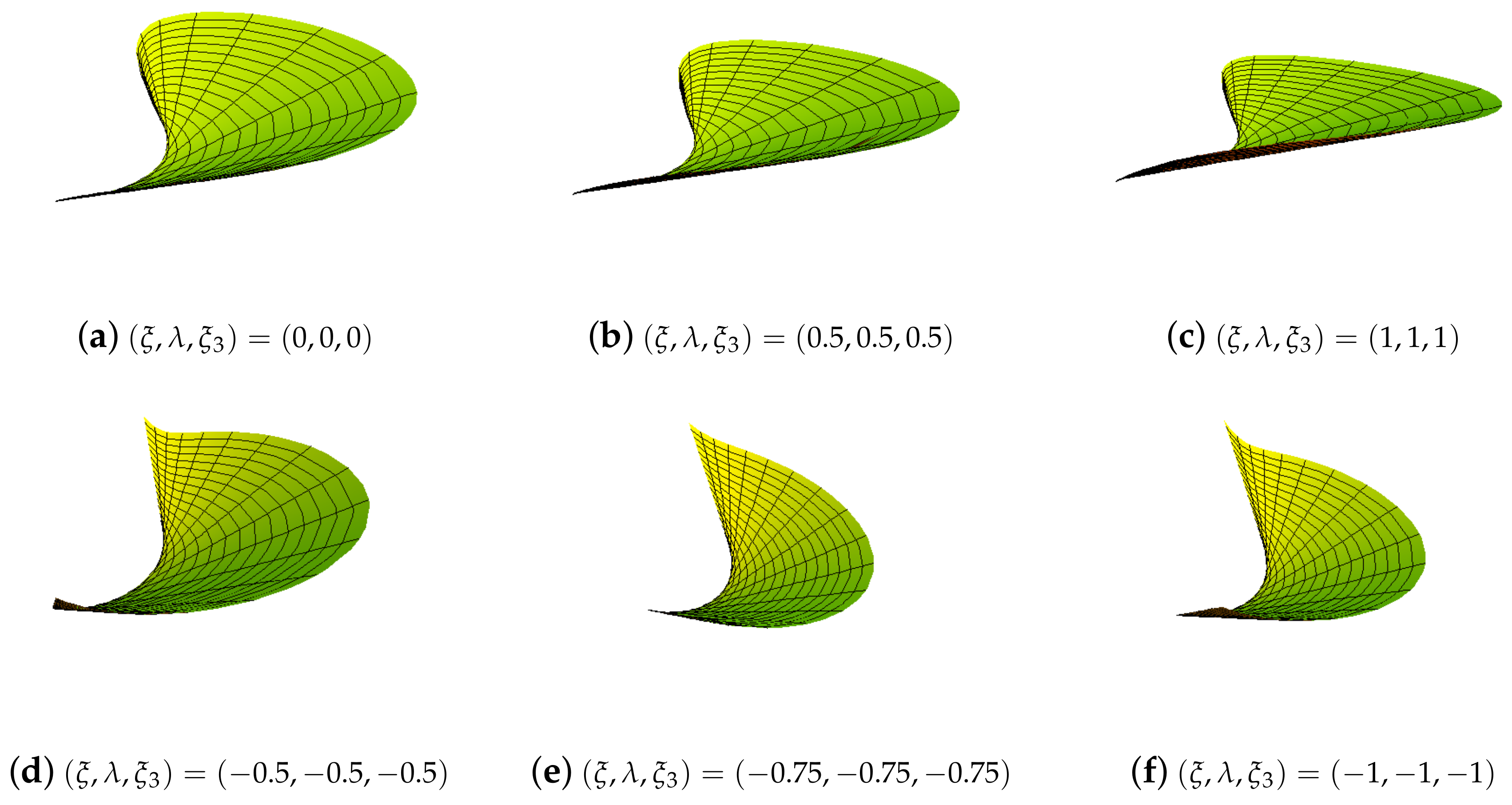
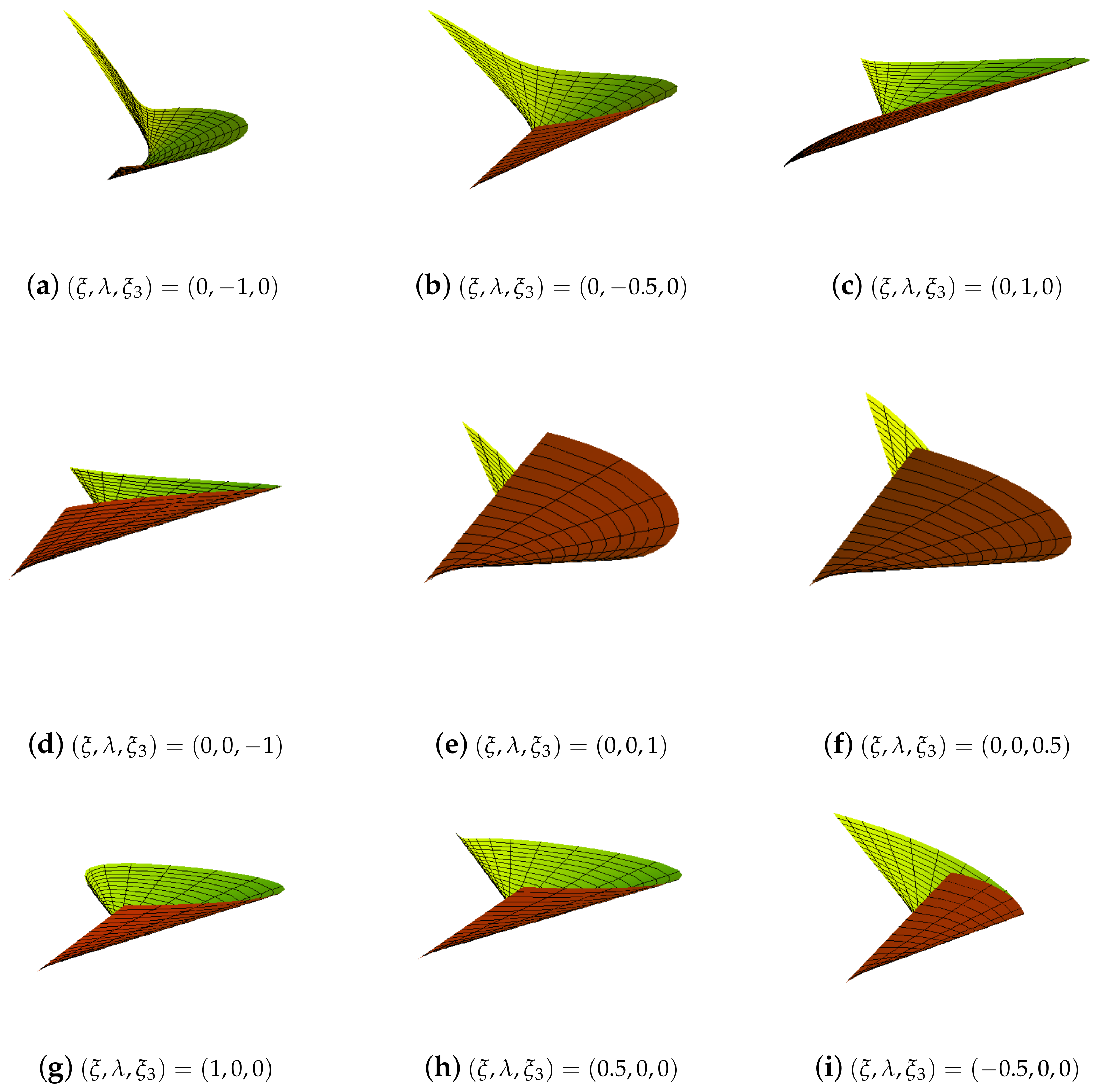
7.1. Examples for the Construction of Enveloping Developable GHT-Bézier Surfaces

In this section, the enveloping developable GHT-Bézier surfaces are shown. For modeling of enveloping developable GHT-Bézier surfaces the center points of four control planes are coplanar and each has an equal distance to the origin. The coordinates of four control planes are given as:

$$\begin{array}{ccc}\hfill {\breve{g}}_0& =& (5\sqrt{2},-5\sqrt{2},5,125),\hfill \\ \hfill {\breve{g}}_1& =& (-5\sqrt{2},-5\sqrt{2},5,125),\hfill \\ \hfill {\breve{g}}_2& =& (-5\sqrt{2},5\sqrt{2},5,125),\hfill \\ \hfill {\breve{g}}_3& =& (5\sqrt{2},5\sqrt{2},5,125).\hfill \end{array}$$

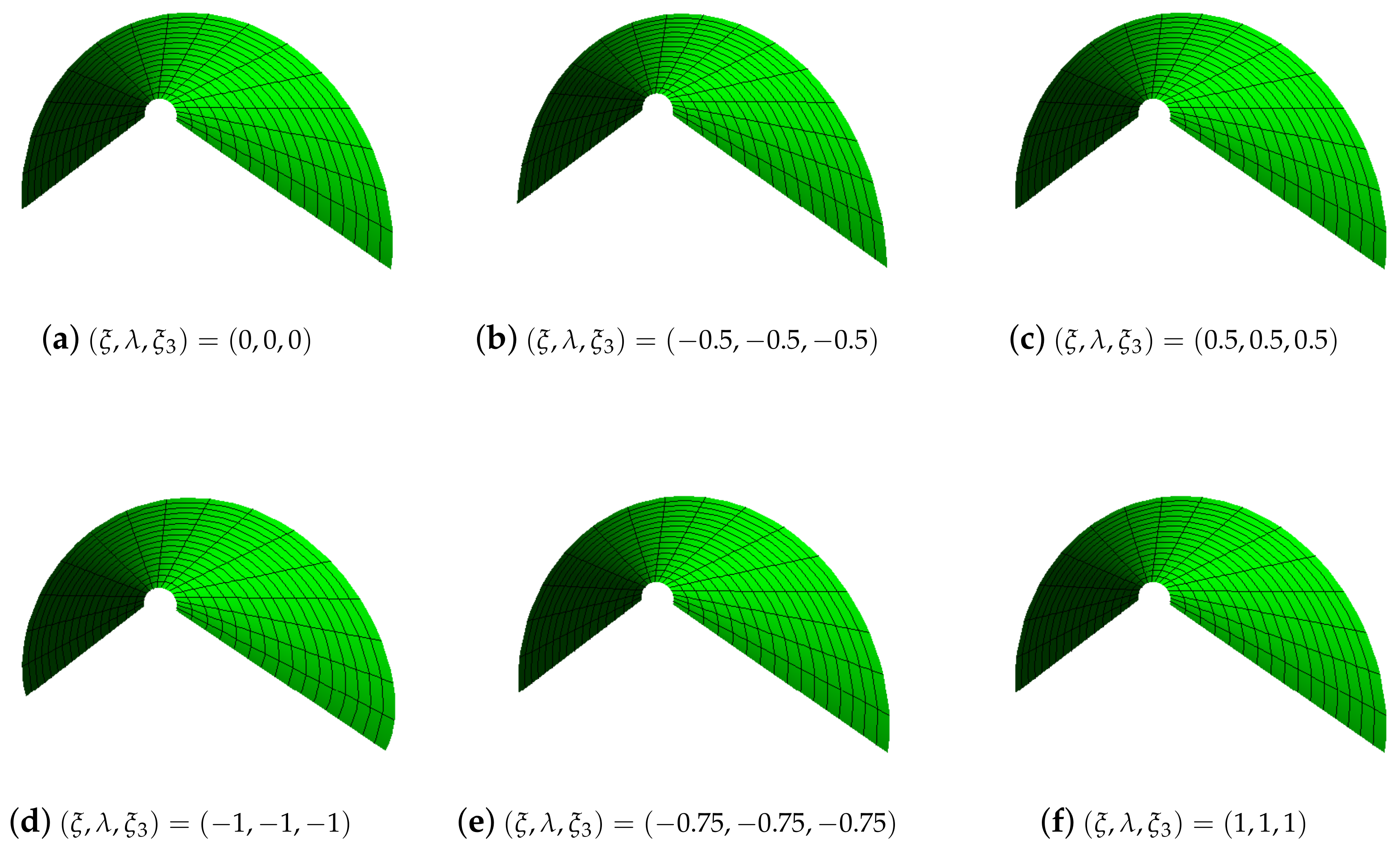
By having different values of shape control parameters $\xi ,\lambda ,{\xi }_3\in [-1,1],$ a class of developable GHT-Bézier surfaces is shown in Figure 3 and Figure 4.

• When all the shape parameters varies equally, then length of starting generator $\alpha (0;\xi ,\lambda ,{\xi }_3)$ and ending generator $\alpha (1;\xi ,\lambda ,{\xi }_3)$ will remain the same, but at the same time the enveloping developable surface as shown in Figure 3 will expand (or shrink).
• When two shape parameters $\xi ,\lambda$ are fixed to 1 and ${\xi }_3$ varies, then length of starting generator $\alpha (0;\xi ,\lambda ,{\xi }_3)$ and ending generator $\alpha (1;\xi ,\lambda ,{\xi }_3)$ are closely related (are same) and enveloping developable GHT-Bézier surface will shrink.
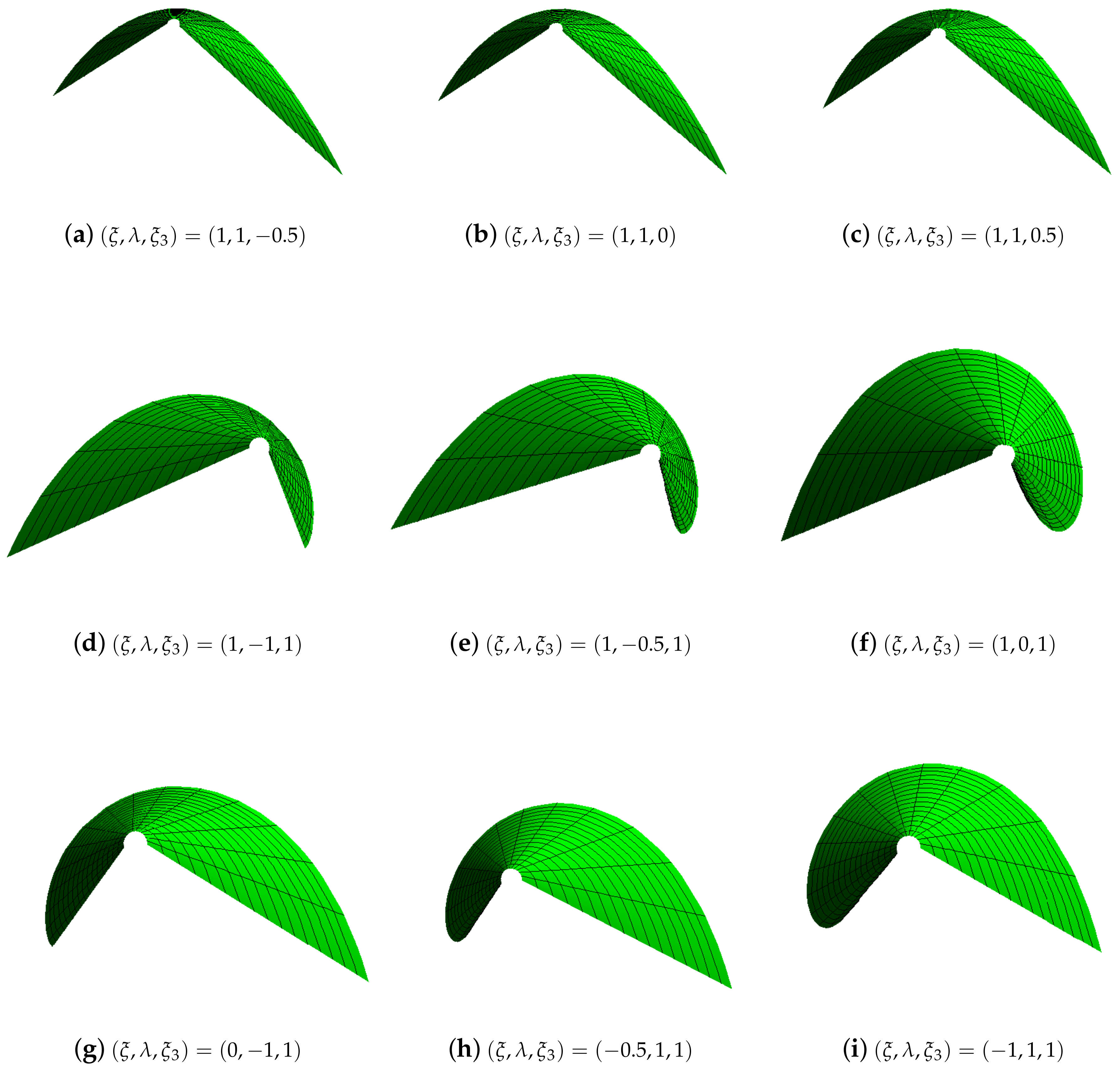
• When shape parameters $\xi ,{\xi }_3$ are fixed to 1 and $\lambda$ varies, then length of starting generator $\alpha (0;\xi ,\lambda ,{\xi }_3)$ is greater then the length of ending generator $\alpha (0;\xi ,\lambda ,{\xi }_3),$ as shown in Figure 4d–f.
• When shape parameters $\lambda ,{\xi }_3$ are fixed to 1 and $\xi$ varies, then length of ending generator $\alpha (1;\xi ,\lambda ,{\xi }_3)$ is greater then the length of starting generator $\alpha (1;\xi ,\lambda ,{\xi }_3)$ and enveloping developable GHT-Bézier surface will expand (or shrink) gradually as shown in Figure 4g–i.

7.2. Spine Curve Developable GHT-Bézier Surface Construction

In this section, a family of spine curve developable GHT-Bézier surfaces is obtained by varying the values of shape parameters. Here we consider the following control planes,

$$\begin{array}{ccc}\hfill {\breve{g}}_0& =& (\frac{13}{2},\frac{13}{2},\frac{13\sqrt{2}}{2},169),\hfill \\ \hfill {\breve{g}}_1& =& (\frac{15}{2},\frac{15}{2},\frac{13\sqrt{2}}{2},225),\hfill \\ \hfill {\breve{g}}_2& =& (-10,-10,10\sqrt{2},400),\hfill \\ \hfill {\breve{g}}_3& =& (\frac{25}{2},\frac{-25}{2},\frac{25\sqrt{2}}{2},625).\hfill \end{array}$$

By taking shape parameters at different values, various shapes of spine curve developable GHT-Bézier surfaces can be constructed. Figure 5 and Figure 6 illustrated the effect of shape parameters in the following manner.

• When we consider all the shape parameters, varies equally with negative values, i.e., $\xi =\lambda ={\xi }_3$ then length of starting generator $\alpha (0;\xi ,\lambda ,{\xi }_3)$ increases with length of ending generator $\alpha (1;\xi ,\lambda ,{\xi }_3),$ but when we have positive values of shape parameters, the length of starting generator decreases with length of ending generator. The behavior of shape parameters will shrink/expand, the shape of the surface as well.
• When two shape parameters $\xi ,{\xi }_3$ are fixed to 0 and $\lambda$ varies, then length of ending generator $\alpha (1;\xi ,\lambda ,{\xi }_3)$ is larger then the length of starting generator $\alpha (0;\xi ,\lambda ,{\xi }_3).$ However, as we increase the values of $\lambda ,$ the surface will shrink and the length of starting generator will also increase.
• When $\xi ,\lambda$ are fixed to 0 and values of ${\xi }_3$ increase, then the length of starting generator $\alpha (0;\xi ,\lambda ,{\xi }_3)$ decreases and length of ending generator $\alpha (1;\xi ,\lambda ,{\xi }_3)$ increases. However, at the same time the spine curve developable GHT-Bézier surface will expand.
• When the shape parameters $\lambda ,{\xi }_3$ are fixed to $0,$ and $\xi$ varies, then the length of starting generator increases and length of ending generator $\alpha (1;\xi ,\lambda ,{\xi }_3)$ remains same. The surface will shrink by decreasing the values of shape parameters.

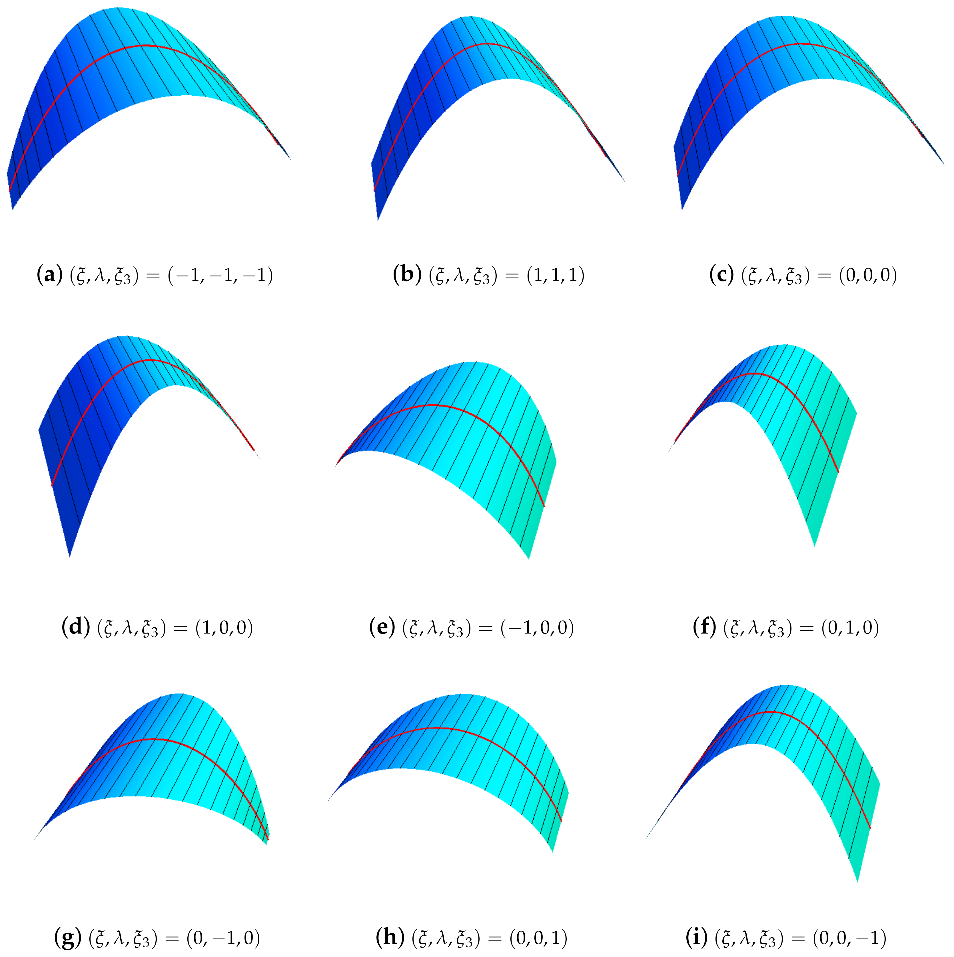
7.3. Designing of Developable Surface Interpolating Geodesic GHT-Bézier Curve with Parameters

In this section, we construct a family of developable surface interpolating geodesic GHT-Bézier curves with different values of shape parameters. By using Equation (16), we consider the value of ${\nu }_2=1,$ and control points for these developable surfaces given as follows:

$$\begin{array}{ccc}\hfill {\breve{g}}_0& =& (0,0,0),\hfill \\ \hfill {\breve{g}}_1& =& (1,0,2),\hfill \\ \hfill {\breve{g}}_2& =& (2,0,2),\hfill \\ \hfill {\breve{g}}_3& =& (3,0,0).\hfill \end{array}$$

Figure 7 shows the effect of shape control parameters on the surfaces in the following manner.

• When shape control parameters $\xi ,\lambda ,{\xi }_3\in [-1,1],$ vary simultaneously, then smooth behavior of surface interpolation geodesic developable surfaces is shown in Figure 7a–c.
• When we fix two shape parameters and vary the remaining shape parameters one by one, then the behavior of developable surfaces also varies and is obvious in Figure 7d–i. The values of shape parameters are mentioned under each figure.

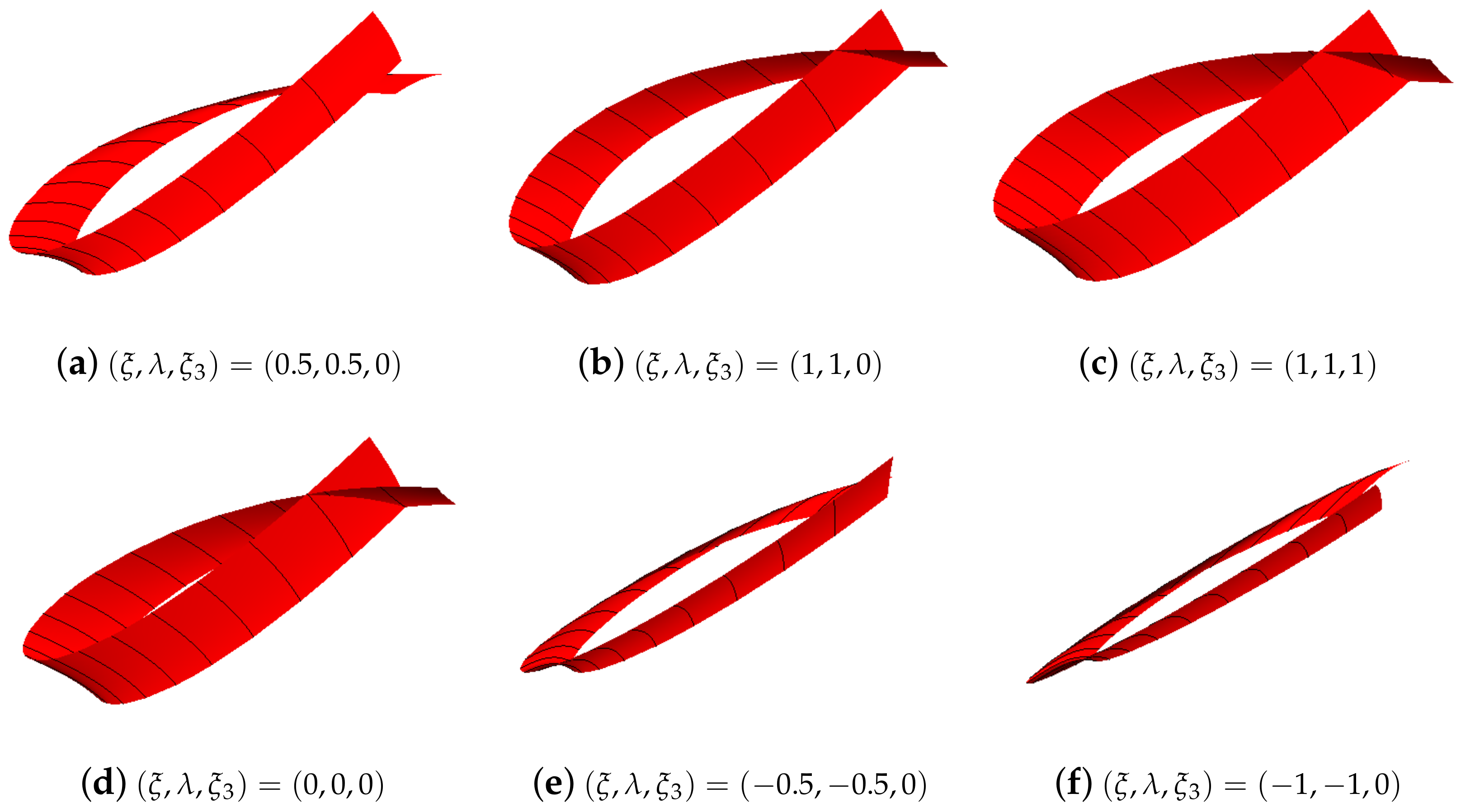
7.4. Construction of Developable GHT-Bézier Canal Surface with Shape Parameters

Canal surfaces are very popular in CAGD. In this section, we want to construct the developable GHT-Bézier canal surfaces geometrically via Mathematica Programme.

Example 1.

Consider a GHT-Bézier curve as defined in Equation (3) having three different shape control parameters. The Frenet frames are taken as,

$$\left\{\begin{array}{c}T\left(\psi \right)=(-sin(\psi ),cos(\psi ),1),\hfill \\ N\left(\psi \right)=(-cos(\psi ),-sin(\psi ),0),\hfill \\ B\left(\psi \right)=(-\frac{1}{2}sin\left(\psi \right),\frac{1}{2}cos\left(\psi \right),-\frac{1}{2}).\hfill \end{array}\right.$$

(39)

The radius function $r\left(\psi \right)={\psi }^2$ and $\sigma \left(\psi \right)=-e^{\psi }.$ Hence, by using Equation (17) the canal surfaces with the control points taken as $\breve{g_0}=(5\sqrt{2},-5\sqrt{2},5),\breve{g_1}=(-5\sqrt{2},-5\sqrt{2},5),\breve{g_2}=(-5\sqrt{2},5\sqrt{2},5),\breve{g_3}=(5\sqrt{2},-5\sqrt{2},5)$ and by varying the values of shape parameters are obvious in Figure 8. The variation in each figure is obvious as we change the shape parameters mentioned under each figure.

Since we know that, the canal surface is the envelope of one parameters family of moving sphere with varying radius, while the developable surface is the envelope of a one-parameter family of planes and we have developed already a theory of Spine curve developable GHT-Bézier surfaces having three shape parameters with GHT-Bernstein basis functions (see Section 4.3 and Section 7.2). Now, based on the theory of developable surfaces by using these GHT-Bernstein basis functions we also constructed developable GHT-Bézier canal surfaces (see Section 4.5 and Example 1). These surfaces play an essential role in descriptive geometry because in the case of an orthographic projection its contour curve can be drawn as the envelope of circles.

7.5. Examples of Smooth Continuity between Two Adjacent Developable GHT-Bézier Surfaces

In CAD/CAM field many products can be obtained by splicing any two developable surfaces with continuity axioms. So, by using continuity conditions described in Section 6, we can construct various complex surfaces. In this section, various examples by using Farin-Boehm $G^2$ continuity, Beta $G^2$ continuity, and by $G^3$ continuity are constructed. Moreover, the effect of shape control parameters on the composite developable GHT-Bézier surfaces are also analyzed.

Example 2.

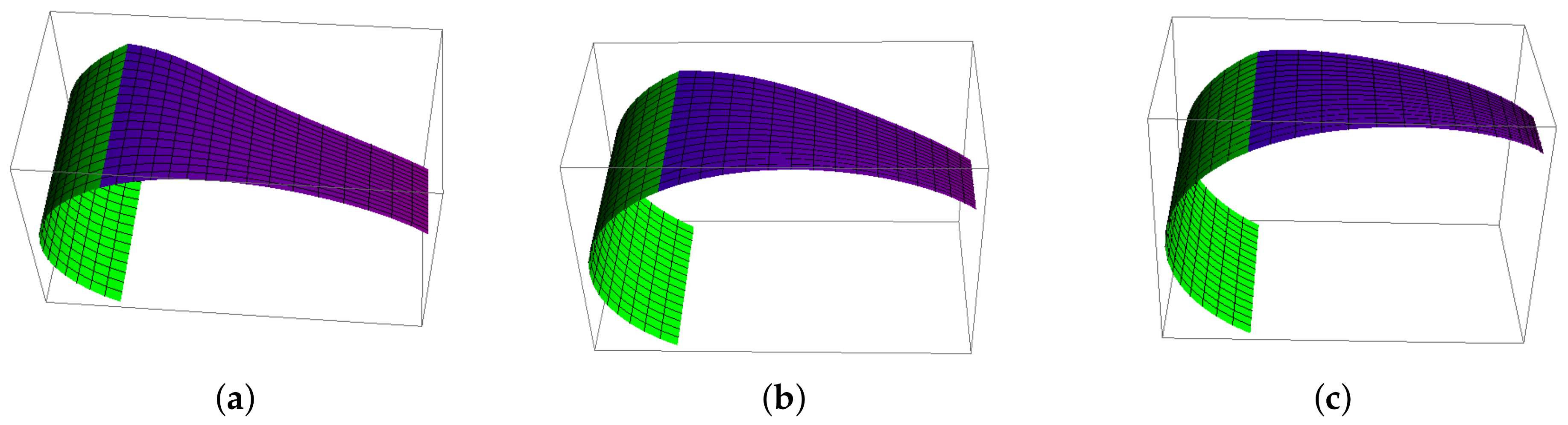
In this example, by having control points and using Farin-Boehm $G^2$ continuity conditions, the developable GHT-Bézier surfaces are given in Figure 9. The values of shape parameters are taken as $(\xi ,\lambda ,{\xi }_3)=(0.1,0,-0.2),$$(\breve{\xi },\breve{\lambda },{\breve{\xi }}_3)=(1,0,-0.2)$ in Figure 9a, $(\xi ,\lambda ,{\xi }_3)=(0,0.1,0),$$(\breve{\xi },\breve{\lambda },{\breve{\xi }}_3)=(1,0,0)$ in Figure 9b and $(\xi ,\lambda ,{\xi }_3)=(0,0.1,0),$$(\breve{\xi },\breve{\lambda },{\breve{\xi }}_3)=(1,0,0.5)$ in Figure 9c. The green surface is the initial developable GHT-Bézier surface, while the purple surface is obtained by the continuity conditions. The control points for initial developable GHT-Bézier surface are given as follows

$$\begin{array}{ccc}\hfill {\breve{g}}_0& =& (0,-20,10,400),\hfill \\ \hfill {\breve{g}}_1& =& (0,-10,10,400),\hfill \\ \hfill {\breve{g}}_2& =& (0,10,20,400),\hfill \\ \hfill {\breve{g}}_3& =& (0,20,10,400),\hfill \end{array}$$

while the control points for final developable GHT-Bézier surface are obtained by Farin-Boehm $G^2$ continuity conditions. The effect of different shape control parameters can be seen in Figure 9a–c.

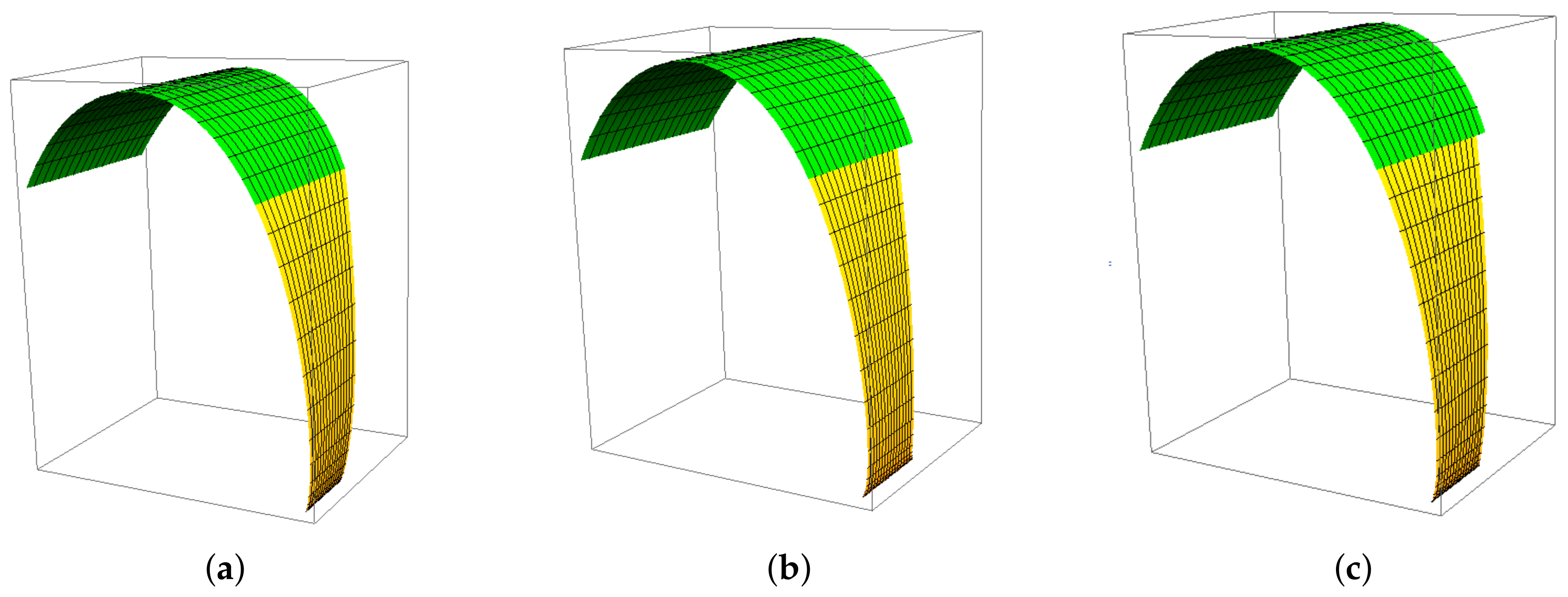
Example 3.

In this example, the developable GHT-Bézier surfaces are constructed by using Beta $G^2$ continuity conditions as shown in Figure 10. The values of shape parameters are taken as $(\xi ,\lambda ,{\xi }_3)=(0.1,0,0.2),$$(\breve{\xi },\breve{\lambda },{\breve{\xi }}_3)=(1,0,0)$, $\gamma =1$ in Figure 10a, $(\xi ,\lambda ,{\xi }_3)=(0.1,0,0.2),$$(\breve{\xi },\breve{\lambda },{\breve{\xi }}_3)=(1,0,0)$, $\gamma =1.1$ in Figure 10b and $(\xi ,\lambda ,{\xi }_3)=(0.1,0,0.2),$$(\breve{\xi },\breve{\lambda },{\breve{\xi }}_3)=(1,0,0)$, $\gamma =1.2$ in Figure 10c. The green surface is the initial developable GHT-Bézier surface, while the yellow surface is the final developable GHT-Bézier surface which is obtained by the continuity conditions. The shape parameters for both surfaces are mentioned under the graph and variation in the shape of the surface is obvious in Figure 10a–c. For Beta $G^2$ continuity, the shape of the surface can also be changed by having different values of scale factor γ.

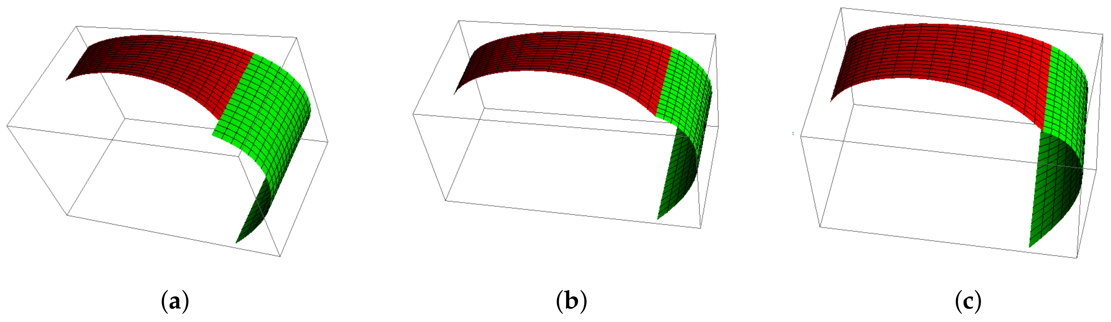
Example 4.

To get more smoothness in the developable GHT-Bézier surfaces, the $G^3$ continuity conditions have been derived. By using the control points as in Example 2 and by $G^3$ continuity conditions, the developable GHT-Bézier surfaces can be obtained as shown in Figure 11. For different shape control parameters and scale factors, the various surfaces can be obtained. The values of shape parameters and scale factors are taken as $(\xi ,\lambda ,{\xi }_3)=(0.5,0,0),$$(\breve{\xi },\breve{\lambda },{\breve{\xi }}_3)=(0.5,0,0),$$\gamma =1.2$ in Figure 11a, $(\xi ,\lambda ,{\xi }_3)=(0.7,0,0),$$(\breve{\xi },\breve{\lambda },{\breve{\xi }}_3)=(0.7,0,0),$$\gamma =1.1$ in Figure 11b and $(\xi ,\lambda ,{\xi }_3)=(0.6,0,0),$$(\breve{\xi },\breve{\lambda },{\breve{\xi }}_3)=(0.6,0,0),$$\gamma =1$ in Figure 11c.

For engineering purposes, the developable surfaces are widely applicable to get numerous complex products such as car bodies, ship designs, and hats, etc. In CAD/CAM, if the apparent surface of a product (such as airplane skin, ship hull and shoes etc.) is a complex developable surface, the surface needs to be considered as a piecewise developable surface composed of multiple ones. Therefore, the continuity conditions between two adjacent GHT-Bézier developable surfaces are presented. By using these continuity conditions the multiple developable surfaces are joined to each other to obtain a complex desired shape, and by changing the values of shape parameters of GHT-Bézier surface the obtained shapes can be slightly modified.

8. Conclusions

As an advancement of classical developable surfaces, a mathematical theory of developable GHT-Bézier surfaces is presented and its application range includes computer vision, computer graphics, multimedia technology, manufacturing industry, and industrial designing, etc. In this paper, a class of GHT-Bernstein basis and GHT-Bézier curve with its basic properties is presented. The graphical representation by varying the values of three different shape parameters is given. The developable GHT-Bézier surfaces are constructed by changing different shape parameters. Numerous complex products are also obtained by using $G^1$ continuity and (Farin-Boehm and Beta) $G^2$ continuity axioms between two adjoining developable GHT-Bézier surfaces. However, the new approach given in this research paper is the derivation of the $G^3$ continuity condition for the construction of the various complex product, and as far as we are aware, it has never been employed for the construction of developable GHT-Bézier surfaces before. Additionally, this derivation could be applied in the future to generate various complex products of developable GHT-Bézier surfaces.

References

- Chu, C.H.; Chen, J.T. Geometric design of developable composite Bézier surfaces. Comput.-Aided Des. Appl. 2004, 1, 531–539. [Google Scholar] [CrossRef] [Green Version]
- Li, C.Y.; Wang, R.H.; Zhu, C.G. Design and G1 connection of developable surfaces through Bézier geodesics. Appl. Math. Comput. 2011, 218, 3199–3208. [Google Scholar] [CrossRef]
- Hu, G.; Cao, X.H.; Qin, X.Q. Geometric design and continuty of developable λ - Bézier surfaces. Adv. Eng. Soft. 2017, 114, 235–245. [Google Scholar] [CrossRef]
- Ammad, M.; Misro, M.Y.; Abbas, M.; Majeed, A. Generalized Developable Cubic Trigonometric Bézier Surfaces. Mathematics 2020, 9, 283. [Google Scholar]
- Zhang, X.W.; Wang, G.J. A new algorithm for designing developable GBT-Bézier surfaces. J. Zhejiang Univ. Sci. 2006, 7, 20506. [Google Scholar] [CrossRef]
- Hu, G.; Junli, W.; Xinqiang, Q. A new approach in designing of local controlled developable H-Bézier surfaces. Adv. Eng. Softw. 2018, 121, 26–38. [Google Scholar] [CrossRef]
- Chen, D.R.; Wang, G.J. Developable GBT-Bézier parametric surfaces. J. Comput. Aided Des. Comput. Graph. 2003, 15, 5705. [Google Scholar]
- Hu, G.; Cao, H.; Wu, J.; Wei, J. Construction of developable surfaces using generalized C-Bézier basis with shape parameters. Comput. Appl. Math. 2020, 39, 1–32. [Google Scholar] [CrossRef]
- Pottmann, H.; Farin, G. Developable rational Bézier and B-spline surfaces. Comput. Aided Geom. Des. 1995, 12, 51331. [Google Scholar] [CrossRef]
- Aumann, G. A simple algorithm for designing developable Bézier surfaces. Comput. Aided Geom. Des. 2003, 20, 601–619. [Google Scholar] [CrossRef]
- Aumann, G. Degree elevation and developable Bézier surfaces. Comput. Aided Geom. Des. 2004, 21, 661–670. [Google Scholar] [CrossRef]
- BiBi, S.; Abbas, M.; Misro, M.Y.; Hu, G. A novel approach of hybrid trigonometric Bézier curve to the modeling of symmetric revolutionary curves and symmetric rotation surfaces. IEEE Access 2019, 7, 165779–165792. [Google Scholar] [CrossRef]
- Qin, X.; Hu, G.; Zhang, N.; Shen, X.; Yang, Y. A novel extension to the polynomial basis functions describing Bézier curve and surfaces of degree n with multiple shape parameters. Appl. Math. Comput. 2013, 223, 1–16. [Google Scholar] [CrossRef]
- González, C.; Albrecht, G.; Paluszny, M.; Lentini, M. Design of C2 algebraic trigonometric Pythagoreans hodograph splies with shape paramneters. Comput. Appl. Math. 2016, 378, 1472–1495. [Google Scholar]
- Wu, X.; Han, X.; Luo, S. Quadratic trigonometric spline curve with shape parameters. In Proceedings of the 2007 10th IEEE International Conference on Computer-Aided Design and Computer Graphics, Beijing, China, 15–18 October 2007; pp. 1–16. [Google Scholar]
- BiBi, S.; Abbas, M.; Miura, K.T.; Misro, M.Y. Geometric Modelling of novel Generalized hybrid Trigonometric Bézier-like curve with Shape Parameters and its Applications. Mathematics 2020, 8, 967. [Google Scholar] [CrossRef]
- BiBi, S.; Abbas, M.; Misro, M.Y.; Majeed, A.; Nazir, T. Construction of Generalized Hybrid Trigonometric Bézier Surfaces with Shape Parameters and Their Applications. J. Math. Imaging Vis. 2021, 1–25. [Google Scholar] [CrossRef]
- Shi, F.Z. Computer Aided Geometric Design and NURBS; China Higher Education Press: Beijing, China, 2001. [Google Scholar]
- Han, X.A.; Ma, Y.; Huang, X. A novel generalization of Bézier curve and surface. J. Comput. Appl. Math. 2008, 217, 180–193. [Google Scholar] [CrossRef] [Green Version]
- Dube, M.; Yadav, B. The quintic trigonometric Bézier curve with single shape parameter. Int. J. Sci. Res. Pub. 2014, 4, 2250–3153. [Google Scholar]
- Ammad, M.; Misro, M.Y. Construction of Local Shape Adjustable Surfaces Using Quintic Trigonometric Bézier Curve. Symmetry 2020, 12, 1205. [Google Scholar] [CrossRef]
- Farin, G. Curves and Surfaces for CAGD. A Practical Guide, 5th ed.; Academic Press: San Diego, CA, USA, 2002. [Google Scholar]
- Juttler, B.; Sampoli, M.L. Hermite interpolation by piecewise polynomial surfaces with rational offsets. Comput. Aided Geom. Des. 2000, 17, 36185. [Google Scholar] [CrossRef]
- Tang, K.; Chen, M. Quasi-developable mesh surface interpolation via mesh deformation. IEEE Trans. Visual. Comput. Graph. 2009, 15, 51828. [Google Scholar]
- Zhou, M.; Peng, G.H.; Ye, Z.L. Design of developable surfaces by using duality between plane and point geometries. J. Comput. Aided Des. Comput. Graph. 2004, 16, 1401–1406. [Google Scholar]
- Zhao, H.Y.; Wang, G.J. A new method for designing a developable surface utilizing the surface pencil through a given curve. Prog. Nat. Sci. 2008, 18, 105–110. [Google Scholar] [CrossRef]
- Chen, M.; Tang, K. G2 quasi-developable GBT-Bézier surface interpolation of two space curves. Comput. Aided Des. 2013, 45, 136577. [Google Scholar] [CrossRef]
- Hwang, H.D.; Yoon, S.H. Constructing developable surfaces by wrapping cones and cylinders. Comput. Aided Des. 2015, 58, 230–235. [Google Scholar] [CrossRef]
- Chung, W.; Kim, S.H.; Shin, K.H. A method for planar development of 3D surfaces in shoe pattern design. J. Mech. Sci. Technol. 2008, 22, 1510–1519. [Google Scholar] [CrossRef]
- Veltkamp, R.C. Survey of continuities of curves and surfgaces. Comput. Graph. Forum. 1992, 11, 93–112. [Google Scholar] [CrossRef] [Green Version]
- Rabinovich, M.; Hoffmann, E.Z.T.; Zurich, E. Discrete Geodesic Nets for Modeling Developable Surfaces. ACM Trans. Graph. 2017, 37, 1–17. [Google Scholar] [CrossRef] [Green Version]
- Qian, J.; Su, M.; Fu, M.; Juan, S.D. Geometric Characterizations of Canal Surfaces in Minkowski 3-Space. Mathematics 2019, 7, 703. [Google Scholar] [CrossRef] [Green Version]
- Tuncer, Y. Canal Surfaces in Galilean 3-Spaces. Kyungpook Math. J. 2017, 57, 319–326. [Google Scholar]
- Valdés, J.N.; Almagro, I.O. Canal surfaces and its application to the CAGD. Am. J. Eng. Res. 2021, 10, 19–31. [Google Scholar]
- Farin, G.E. Curves and Surfaces for CAGD; Morgan Kaufmann Publishers: San Francisco, CA, USA, 2002. [Google Scholar]
- Fu, X.; Jung, S.D.; Qian, J.; Su, M. Gometric characterization of canal surfaces in Minkowski 3-space. I. Bull. Korean Math. Soc. 2019, 56, 867–883. [Google Scholar]
- Xu, Z.Q.; Feng, R.Z.; Sun, J.G. Analytic and algebraic properties of canal surfaces. Appl. Math. Comput. 2016, 195, 220–228. [Google Scholar] [CrossRef] [Green Version]
- Cho, H.C.; Choi, H.I.; Kwon, S.H.; Lee, D.S.; Wee, N.S. Clifford algebra, Lorentzian geometry, and rational parametrization of canal surfaces. Comput. Aided Geom. 2004, 21, 327–339. [Google Scholar] [CrossRef]
Figure 1.
Plots of p degree GHT-Bernstein basis functions.
Figure 2.
GHT-Bézier curves by multiple shape parameters.
Figure 3.
Enveloping developable GHT-Bézier surfaces, having same values of .
Figure 4.
Enveloping developable GHT-Bézier surfaces, having different values of .
Figure 5.
Spine curve developable GHT-Bézier surfaces having same values of .
Figure 6.
Graphical representation of Spine curve developable GHT-Bézier surfaces, having different values of .
Figure 7.
Surface interpolation geodesic developable GHT-Bézier surfaces having different values of .
Figure 8.
Graphical representation of Developable GHT-Bézier canal surfaces with different shape parameters.
Figure 9.
Farin-Boehm continuity of developable GHT-Bézier surfaces.
Figure 10.
Beta continuity of developable GHT-Bézier surfaces.
Figure 11.
continuity of developable GHT-Bézier surfaces.
Publisher’s Note: MDPI stays neutral with regard to jurisdictional claims in published maps and institutional affiliations. |
© 2021 by the authors. Licensee MDPI, Basel, Switzerland. This article is an open access article distributed under the terms and conditions of the Creative Commons Attribution (CC BY) license (https://creativecommons.org/licenses/by/4.0/).
Share and Cite
MDPI and ACS Style
BiBi, S.; Misro, M.Y.; Abbas, M.; Majeed, A.; Nazir, T. G3 Shape Adjustable GHT-Bézier Developable Surfaces and Their Applications. Mathematics 2021, 9, 2350. https://0-doi-org.brum.beds.ac.uk/10.3390/math9192350
AMA Style
BiBi S, Misro MY, Abbas M, Majeed A, Nazir T. G3 Shape Adjustable GHT-Bézier Developable Surfaces and Their Applications. Mathematics. 2021; 9(19):2350. https://0-doi-org.brum.beds.ac.uk/10.3390/math9192350
Chicago/Turabian StyleBiBi, Samia, Md Yushalify Misro, Muhammad Abbas, Abdul Majeed, and Tahir Nazir. 2021. "G3 Shape Adjustable GHT-Bézier Developable Surfaces and Their Applications" Mathematics 9, no. 19: 2350. https://0-doi-org.brum.beds.ac.uk/10.3390/math9192350
Note that from the first issue of 2016, this journal uses article numbers instead of page numbers. See further details here.