Existence and Uniqueness of Nontrivial Periodic Solutions to a Discrete Switching Model

Abstract

To control the spread of mosquito-borne diseases, one goal of the World Mosquito Program’s Wolbachia release method is to replace wild vector mosquitoes with Wolbachia-infected ones, whose capability of transmitting diseases has been greatly reduced owing to the Wolbachia infection. In this paper, we propose a discrete switching model which characterizes a release strategy including an impulsive and periodic release, where Wolbachia-infected males are released with the release ratio ${\alpha }_1$ during the first N generations, and the release ratio is ${\alpha }_2$ from the $(N+1)$-th generation to the T-th generation. Sufficient conditions on the release ratios ${\alpha }_1$ and ${\alpha }_2$ are obtained to guarantee the existence and uniqueness of nontrivial periodic solutions to the discrete switching model. We aim to provide new methods to count the exact numbers of periodic solutions to discrete switching models.

1. Introduction

The global incidence of dengue is placing more than 50% of the world’s population at risk, and affects more than 100 countries around the world [1]. As a mosquito-borne disease, dengue viruses are transmitted through the bites of infected Aedes female mosquitoes, including Aedes aegypti and Aedes albopictus, which act as the main vectors of dengue. There are four serotypes of dengue viruses. As the repeated proof of the antibody-dependent enhancement phenomenon between different serotypes, the application of the dengue vaccine has been halted [2,3]. Furthermore, no effective drugs are available for dengue viruses, especially for severe cases, including dengue hemorrhagic fever and dengue shock syndrome. Hence, the most straightforward way to control dengue is to eradicate mosquitoes by spraying insecticide or removing mosquito breeding sites, but neither method works effectively due to the appearance of insecticide resistance and difficulty in eradicating breeding sites [4].

Luckily, the World Mosquito Program’s Wolbachia release method is helping communities worldwide to control and prevent the spread of mosquito-borne diseases. The endosymbiotic bacteria Wolbachia occurs naturally in 60% of insect species, which are safe for humans and the environment. As the successful establishment of Wolbachia in Aedes mosquitoes through microinjection [5,6], Wolbachia-driven mosquito control techniques have become one of the effective biological control methods. The Wolbachia bacteria is maternally inherited, which can induce a special mechanism called “cytoplasmic incompatibility”(CI), resulting in early developmental arrest of the embryo when infected male mosquitoes mate with uninfected female mosquitoes [5,6,7,8,9]. By using CI, and the maternal transmission of Wolbachia, one of the World Mosquito Program’s Wolbachia release methods aims to replace the wild vector mosquitoes with Wolbachia infected ones, whose capability of transmitting diseases has been greatly reduced owing to the Wolbachia infection [5,6,7,8,9]. Taking the release in Australia as an example, back to 2011, Wolbachia-infected mosquitoes were released to replace the natural Aedes populations in Cairns, reaching a near-fixation of Wolbachia in a few months [9,10]. Similar field trials have also been carried out in Brazil, Vietnam, Indonesia, etc. Post surveillance has shown that in areas where Wolbachia is self-sustaining at a high level, there have been no dengue outbreaks.

Prior to area-wide releases, cage experiments are essential for designing effective and affordable release strategies. Motivated by the experimental observation in [7] that supplemental male release in every generation can accelerate the Wolbachia invasion, we develop a general discrete model which is based on the classic models in [11,12,13,14,15,16], which focused on Wolbachia spread dynamics in cage mosquito populations without supplemental releases. All these discrete models only include a one-time release of both Wolbachia-infected females and males, which generated an unstable equilibrium, below which the Wolbachia infections will disappear, and above which, Wolbachia invasion is successful.

The generalized model developed in Section 2 covers the models in [11,12,13,14,15,16] as special cases. Particularly, we focus on a periodic and impulsive release strategy, where Wolbachia-infected males are released with the release ratio ${\alpha }_1$ during the first N generations, and the release ratio from generation $N+1$ to generation T is ${\alpha }_2$. This leads to a discrete switching model. Very recently, this release strategy was investigated thoroughly, in [17,18,19], by using ordinary differential equation models, leaving the study of discrete models, which are well suited for cage experiment absence. In Section 3, sufficient conditions to guarantee the existence of at least one T-periodic solution are obtained for the discrete switching model. Although our numerical example shows that the T-periodic solution is also unique when it exists, we failed to prove it theoretically for general N and T, and methods used in [17,18,19] are not applicable for discrete models. However, we only succeed to prove that this numerical observation holds for the special case $N=1$ and $T=2$. The whole paper is enveloped with a brief discussion about the insight of our main results in Section 4.

2. Model Development

Motivated on experimental observations in [5,6,7,8,9], and our previous works [20,21,22,23], we assume that (i) the maternal leakage rate is $\mu$: among offspring from infected females, where $1-\mu$ of them are infected, and $\mu$ of them are uninfected; (ii) CI intensity is $s_h$: among eggs produced from wild pregnant female mosquitoes mated with infected males, $s_h$ of them will not hatch, and the hatch rate of other three compatible crosses is 1; (iii) equal sex determination: the birth ratio of male-to-female is 1:1, irrelevant of their mothers infection status. Thus, we assume that at the n-th generation, the number of infected female/male mosquitoes is $I_n$, and the number of uninfected female/male mosquitoes is $U_n$. The infection frequency is then defined by $x_n=I_n/(I_n+U_n)$. At the $n+1$-th generation, the dynamic of the mosquitoe population is interfered upon by the supplemental release of infected males, whose abundance is assumed to be $m_n(I_n+U_n)$. Here, $m_n$ can be interpreted as the release ratio of released males to the total number of female or male mosquitoes.

Although the supplemental release of the infected males causes temporary biased male-to-female ratios at the n-th generation, we assume that the sex ratio of the newly borne population at the $(n+1)$-th generation is 1:1, due to the assumption of equal sex determination. With the release of these infected males, the production rate, as well as the infection frequency, is reduced. Since infected females are not supplementally released, the proportions of infected and uninfected females at the n-th generation are still $x_n$ and $1-x_n$, respectively. With $m_n(I_n+U_n)$ infected males added at the n-th generation, the proportion of infected males goes from $x_n$ to:

$$\frac{I_n+m_n(I_n+U_n)}{I_n+U_n+m_n(I_n+U_n)}=\frac{x_n+m_n}{1+m_n},$$

and the proportion of uninfected males goes from $1-x_n$ to:

$$\frac{U_n}{I_n+U_n+m_n(I_n+U_n)}=\frac{1-x_n}{1+m_n}.$$

At the $(n+1)$-th generation, the infection status of infected offspring is independent on the male partner’s infection status, the proportion of infected individuals is $(1-\mu )(1-s_f)x_n$, where $s_f$ represents the fitness cost of infected females relative to uninfected ones, that is, if the fitness of Wolbachia-free mosquitoes is 1, then the fitness of infected mosquitoes is reduced to $1-s_f$. We should mention here, that in our model, $s_f$ counts the fitness costs caused by Wolbachia infection, such as fecundity reduction, egg viability, hatch rate decrease, and mean longevity [5,6,7,8,9]. Meanwhile, the maternal transmission leakage rate $\mu$ reduces the proportion of infected mosquitoes from $(1-s_f)x_n$ to $(1-\mu )(1-s_f)x_n$. And the contribution of infected mothers to uninfected proportion is $\mu (1-s_f)x_n$.

On the uninfected offspring, we need to consider CI. Under the random mating assumption [11,13,14,16], the mating probability for a female mating with an uninfected male is $\frac{1-x_n}{1+m_n}$, and the hatch rate is 1, which is reduced to $1-s_h$ if the father is infected, with the mating probability then being $\frac{x_n+m_n}{1+m_n}$. Hence, the contribution of uninfected mothers to the proportion of uninfected mosquitoes at the $(n+1)$-th generation is:

$$(1-s_h)(1-x_n)\frac{x_n+m_n}{1+m_n}+(1-x_n)\frac{1-x_n}{1+m_n}.$$

To sum up, we have our general model as:

$$x_{n+1}=\frac{(1-\mu )(1-s_f)(1+m_n)x_n}{s_h{x}_n^2-\left(s_f+s_h+m_n(s_f-s_h)\right)x_n+1+(1-s_h)m_n},$$

(1)

with $n=1,2,\dots$.

The generalized model (1) covers the models in [11,12,13,14,15,16] as special cases. For example, the first discrete model studying Wolbachia infection frequency with laboratory data and parameters was developed in 1959 by Caspari and Watson [11], who were motivated by the CI mechanism in mosquitoes. The model in [11] is a special case of model (1) with $\mu =0$ and $m_n\equiv 0$, which produces an unstable equilibrium point $s_f/s_h$ such that only when the initial infection frequency surpasses $s_f/s_h$ can Wolbachia invasion be guaranteed. After that, the discrete model for Wolbachia spread dynamics has been put on the shelf for more than 15 years until 1975. Fine [12,13] observed the maternal leakage from Wolbachia-infected mothers and introduced the maternal leakage rate $\mu$ into the model in [11] as the third crucial parameter. Again, the model in [12,13] is a special case of model (1) with $m_n\equiv 0$. For $m_n\equiv 0$, since the 1990’s, systematic studies have been carried out by Hoffmann and Turelli on Wolbachia spread dynamics in Drosophila simulans [14,15,16]. The dynamics can be completely determined by the position of the unstable equilibrium frequency, which can be explicitly expressed in terms of $s_f$, $s_h$ and $\mu$. Once prior information on $s_f$, $s_h$ and $\mu$ is known, the unstable equilibrium frequency determines the fate of the Wolbachia invasion. After that, discrete models in [11,12,13,14,15,16] have been seldom revisited due to their clear dynamics, until 2019, when we introduced the notion of supplementary releases into the discrete model [24] for the first time, as in model (1), with $m_n\equiv \alpha$.

Although model (1) is simple in its form, it can generate much richer dynamics than the models in previous works. In the current work, we begin with the easiest case with $s_h=1$ and $\mu =0$, i.e., the CI is complete and the maternal transmission is perfect. In this case, model (1) is reduced to:

$$x_{n+1}=\frac{(1-s_f)(1+m_n)x_n}{x_n^2-\left[1+s_f-m_n(1-s_f)\right]x_n+1},$$

(2)

with $n=1,2,\dots$. Particularly, when $m_n\equiv \alpha$, model (2) is further reduced to:

$$\mathsf{\Delta }{x}_n=x_{n+1}-x_n=\frac{x_n(1-x_n)\left[x_n+\alpha (1-s_f)-s_f\right]}{x_n^2-\left[1+s_f-\alpha (1-s_f)\right]x_n+1},n=1,2,\dots .$$

(3)

By defining:

$${\alpha }^{*}=\frac{s_f}{1-s_f},$$

From Theorems 3.1–3.3 in [24] with $\mu =0$ and $s_h=1$, we can obtain the following lemma.

Lemma 1 

([24]). For $\alpha \ge 0$, model (3) has a zero equilibrium point $x_0^{*}=0$ and a Wolbachia fixation equilibrium point $x_1^{*}=1$. Furthermore,

(1)

When $\alpha \in [0,{\alpha }^{*})$, model (3) has an unstable equilibrium point $\widehat{x}\left(\alpha \right)=s_f-\alpha (1-s_f)$, which serves as a threshold value on the initial frequency $x_1$: if $x_1\in (0,\widehat{x}\left(\alpha \right))$, then $x_n\to 0$ as $n\to \infty$, whereas for $x_1\in (\widehat{x}\left(\alpha \right),1)$, $x_n\to 1$ as $n\to \infty$.

(2)

When $\alpha \ge {\alpha }^{*}$, we have $\mathsf{\Delta }{x}_n>0$ for any $x_1\in (0,1)$, i.e., the equilibrium $x_1^{*}=1$ is globally asymptotically stable.

Here, we aim to study the case that a periodic and impulsive release strategy, in each release period T, Wolbachia-infected male mosquitoes are released with $m_n={\alpha }_1$ during the first N generations for $n\in Z(1+kT,kT+N)$, and $m_n={\alpha }_2$ for $n\in Z(kT+N+1,(k+1\left)T\right)$. Then the model switches between:

$$x_{n+1}=\frac{(1-s_f)(1+{\alpha }_1)x_n}{x_n^2-[1+s_f-{\alpha }_1(1-s_f)]x_n+1}:=F\left(x_n\right),$$

(4)

for $n\in Z(1+kT,kT+N)$, and:

$$x_{n+1}=\frac{(1-s_f)(1+{\alpha }_2)x_n}{x_n^2-[1+s_f-{\alpha }_2(1-s_f)]x_n+1}:=G\left(x_n\right),$$

(5)

for $n\in Z(kT+N+1,(k+1\left)T\right)$. We assume that ${\alpha }_2<{\alpha }_1$ holds without loss of generality throughout the paper.

It’s easy to see that when ${\alpha }_2\ge {\alpha }^{*}$, we get $\mathsf{\Delta }{x}_n>0$. Therefore, for any $x_1\in (0,1)$, $\left\{x_n\right\}$ is strictly monotonously increasing to 1, and we can reach our first result as follows.

Theorem 1. 

When ${\alpha }_2\ge {\alpha }^{*}$, the trivial equilibrium 0 of model (4) and (5) is unstable, and Wolbachia fixation equilibrium point 1 is globally asymptotically stable.

3. At Least One Nontrivial $\mathbf{T}$-Periodic Solution to (4) and (5)

Let ${\left\{x_n\right\}}_{n=1}^{\infty }:={\left\{x_n(1,u)\right\}}_{n=1}^{\infty }$ denote the solution of model (4) and (5) with initial value $x_1=u>0$. Then ${\left\{x_n\right\}}_{n=2}^{N+1}$ satisfies (4) with the initial value $x_1=u$ and $x_2=F\left(u\right)$, which offers:

$$\overline{h}\left(u\right):=x_{N+1}=F^{\left(N\right)}\left(u\right)$$

(6)

by induction. Initiated from $x_{N+1}$, ${\left\{x_n\right\}}_{n=N+2}^{T+1}$ satisfies (5) with $x_n=G^{(n-N-1)}\left(x_{N+1}\right).$ Hence,

$$h\left(u\right):=x_{T+1}=G^{(T-N)}\left(x_{N+1}\right)=G^{(T-N)}\left(\overline{h}\left(u\right)\right)=G^{(T-N)}\left(F^{\left(N\right)}\left(u\right)\right).$$

(7)

Thus, the dynamics of model (4) and (5) depends on the switching frquency between Equations (4) and (5). If models (4) and (5) have a T-periodic solution initiated from u, then $h\left(u\right)=u$. Therefore, finding the periodic solutions of models (4) and (5) is equivalent to finding the fixed points of h. From (6), (7), and the facts that $F\left(0\right)=G\left(0\right)=0$ and $F\left(1\right)=G\left(1\right)=1$, we get:

$$h\left(0\right)=\overline{h}\left(0\right)=0,h\left(1\right)=\overline{h}\left(1\right)=1,$$

(8)

which means that 0 and 1 are two fixed points of h, or equivalently, models (4) and (5) has 0 and 1 as two trivial T-periodic solutions.

Next, we seek sufficient conditions to guarantee that models (4) and (5) have at least one nontrivial T-periodic solution. We begin with the case ${\alpha }_2<{\alpha }_1<{\alpha }^{*}$.

In this case, Lemma 1 implies that both (4) and (5) produce bistable dynamics with the existence of unstable equilibrium points, denoted by $\widehat{x}\left({\alpha }_1\right)$ and $\widehat{x}\left({\alpha }_2\right)$ with $\widehat{x}\left({\alpha }_i\right)=s_f-{\alpha }_i(1-s_f)$ for $i=1,2$, respectively. Since ${\alpha }_1>{\alpha }_2$, we reach $\widehat{x}\left({\alpha }_1\right)<\widehat{x}\left({\alpha }_2\right)$. Furthermore, Lemma 1 implies that,

$$\begin{array}{cc}\hfill & \overline{h}\left(u\right)\le u,h\left(u\right)<\overline{h}\left(u\right)\Rightarrow h\left(u\right)<u,\mathrm{for}u\in (0,\widehat{x}\left({\alpha }_1\right)],\hfill \\ \hfill & \overline{h}\left(u\right)>u,h\left(u\right)\ge \overline{h}\left(u\right)\Rightarrow h\left(u\right)>u,\mathrm{for}u\in [\widehat{x}\left({\alpha }_2\right),1).\hfill \end{array}$$

(9)

The continuity of $h\left(u\right)$ in u guarantees that h has at least one fixed point in $(\widehat{x}\left({\alpha }_1\right),\widehat{x}\left({\alpha }_2\right))$. Therefore, we have:

Lemma 2. 

When ${\alpha }_2<{\alpha }_1<{\alpha }^{*}$, model (4) and (5) has at least one nontrivial T-periodic solution initiated from $(\widehat{x}\left({\alpha }_1\right),\widehat{x}\left({\alpha }_2\right))$.

For the case ${\alpha }_2<{\alpha }^{*}\le {\alpha }_1$, similarly from Lemma 1, we have:

$$\overline{h}\left(u\right)>u,h\left(u\right)\ge \overline{h}\left(u\right)\Rightarrow h\left(u\right)>u,\mathrm{for}u\in [\widehat{x}\left({\alpha }_2\right),1).$$

(10)

However, the sign of $h\left(u\right)-u$ is indefinite for $u\in (0,\widehat{x}\left({\alpha }_2\right))$. This leads us to calculate $h^{\prime }\left(0\right)$. Since $h\left(0\right)=0$, we reach:

$$h^{\prime }\left(0\right)=\underset{u\to 0}{lim}\frac{h\left(u\right)}{u}=\underset{u\to 0}{lim}\frac{h\left(u\right)}{\overline{h}\left(u\right)}·\frac{\overline{h}\left(u\right)}{u},$$

(11)

where:

$$\underset{u\to 0}{lim}\frac{\overline{h}\left(u\right)}{u}=\underset{u\to 0}{lim}\frac{F^{\left(N\right)}\left(u\right)}{F^{(N-1)}\left(u\right)}·\frac{F^{(N-1)}\left(u\right)}{F^{(N-2)}\left(u\right)}\dots \frac{F\left(u\right)}{u}.$$

(12)

Since:

$$\underset{u\to 0}{lim}\frac{F^{\left(i\right)}\left(u\right)}{F^{(i-1)}\left(u\right)}=\underset{u\to 0}{lim}\frac{F\left(F^{(i-1)}\left(u\right)\right)}{F^{(i-1)}\left(u\right)}=\frac{(1-s_f)(1+{\alpha }_1)F^{(i-1)}\left(u\right)}{F^{(i-1)}\left(u\right)}=(1-s_f)(1+{\alpha }_1),$$

for $i=1,2,\dots ,N$ with $F^{\left(0\right)}\left(u\right)=u$. Therefore, from (12),

$$\underset{u\to 0}{lim}\frac{\overline{h}\left(u\right)}{u}={(1-s_f)}^N{(1+{\alpha }_1)}^N.$$

(13)

Similarly,

$$\begin{array}{cc}\hfill \underset{u\to 0}{lim}\frac{h\left(u\right)}{\overline{h}\left(u\right)}=& \underset{u\to 0}{lim}\frac{G^{(T-N)}\left(\overline{h}\left(u\right)\right)}{G^{(T-N-1)}\left(\overline{h}\left(u\right)\right)}·\frac{G^{(T-N-1)}\left(\overline{h}\left(u\right)\right)}{G^{(T-N-2)}\left(\overline{h}\left(u\right)\right)}\dots \frac{G\left(\overline{h}\left(u\right)\right)}{\overline{h}\left(u\right)}\hfill \\ \hfill =& {(1-s_f)}^{T-N}{(1+{\alpha }_2)}^{T-N}.\hfill \end{array}$$

(14)

Hence, combining (11), (13), and (14), we have:

$$h^{\prime }\left(0\right)=\underset{u\to 0}{lim}\frac{h\left(u\right)}{u}={(1-s_f)}^T{(1+{\alpha }_1)}^N{(1+{\alpha }_2)}^{T-N},$$

which implies that when ${\alpha }_1,{\alpha }_2$ lie in:

$$D=\left\{({\alpha }_1,{\alpha }_2)|{(1+{\alpha }_1)}^N{(1+{\alpha }_2)}^{T-N}<\frac{1}{{(1-s_f)}^T}\right\},$$

(15)

we have $h^{\prime }\left(0\right)<1$. Therefore, there exists $\delta >0$ such that:

$$h\left(u\right)<u,\mathrm{for}u\in (0,\delta ),$$

(16)

where $\delta$ is sufficiently small. Recalling that $h\left(\widehat{x}\left({\alpha }_2\right)\right)>\widehat{x}\left({\alpha }_2\right)$, there exists at least one $u^{*}\in [\delta ,\widehat{x}\left({\alpha }_2\right))$ such that:

$$h\left(u^{*}\right)=u^{*},h^{\prime }\left(u^{*}\right)\ge 1,\mathrm{and}h\left(u\right)<u\mathrm{for}u\in (0,u^{*}).$$

The above analysis leads to another sufficient condition for the existence of nontrivial T-periodic solutions to the models (4) and (5) as follows.

Lemma 3. 

If $({\alpha }_1,{\alpha }_2)\in D$ and ${\alpha }_2<{\alpha }^{*}\le {\alpha }_1$, then models (4) and (5) have at least one nontrivial T-periodic solution with u lying in $[\delta ,\widehat{x}\left({\alpha }_2\right))$, where δ is defined in (16).

Combining the results shown in Lemmas 2 and 3, sufficient conditions to guarantee the existence of nontrivial T-periodic solutions to the models (4) and (5) are stated as follows.

Theorem 2. 

Models (4) and (5) have at least one nontrivial T-periodic solution, if one of the following two conditions holds,

$$\left(\mathrm{i}\right){\alpha }_2<{\alpha }_1<{\alpha }^{*},\left(\mathrm{ii}\right){\alpha }_2<{\alpha }^{*}\le {\alpha }_1\mathrm{and}({\alpha }_1,{\alpha }_2)\in D,$$

(17)

where D is defined in (15).

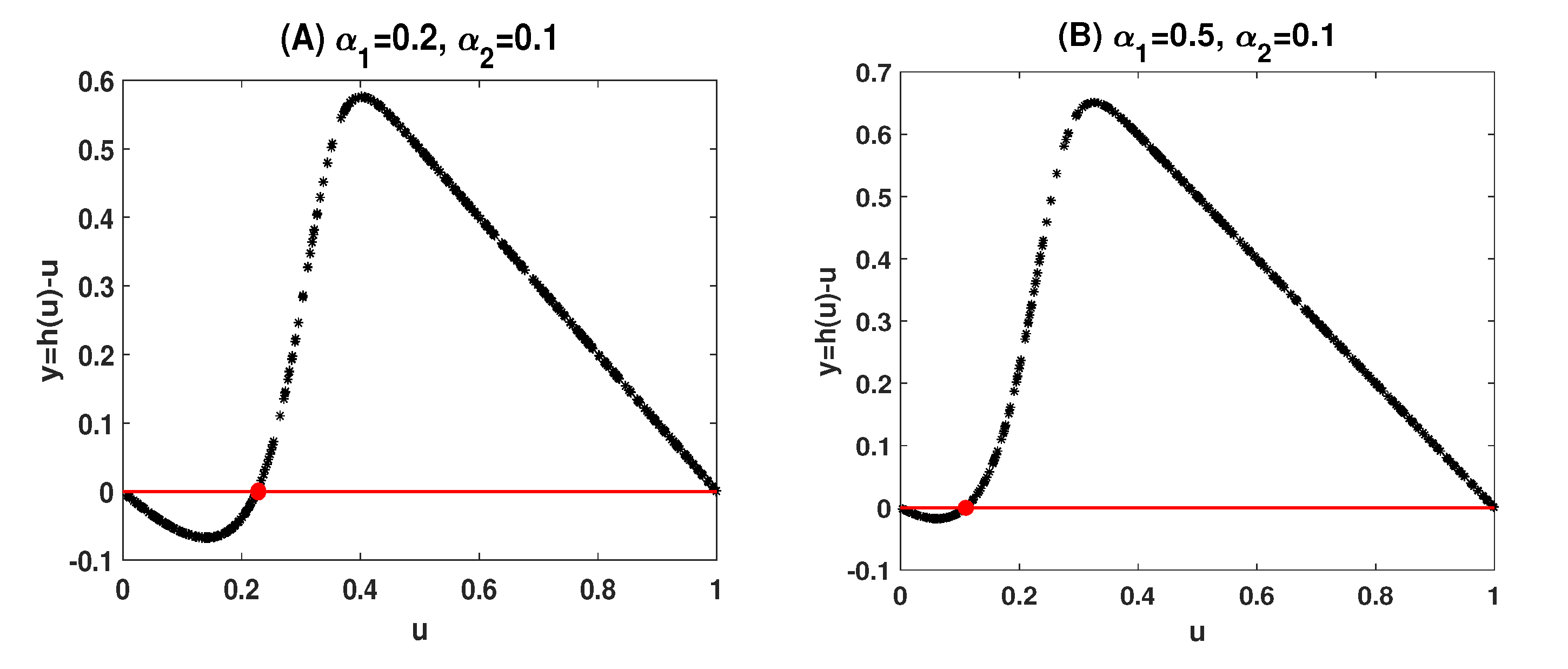
The following example displays that when the conditions in (17) hold, the T-periodic solution not only exists, but also may be unique.

Example 1. 

Let $s_f=0.3$. Then ${\alpha }^{*}=\frac{s_f}{1-s_f}\approx 0.4286$. When we take $N=2$ and $T=5$, models (4) and (5) read:

$$x_{n+1}=\left\{\begin{array}{cc}\frac{0.7(1+{\alpha }_1)x_n}{x_n^2-(1.3-0.7{\alpha }_1)x_n+1},& n\in Z(5k+1,5k+2),\\ \frac{0.7(1+{\alpha }_2)x_n}{x_n^2-(1.3-0.7{\alpha }_2)x_n+1},& n\in Z(5k+3,5(k+1\left)\right).\end{array}\right.$$

(18)

Letting ${\alpha }_1=0.2$ and ${\alpha }_2=0.1$. Then (i) in (17) holds. By randomly selecting 400 points for $u\in [0,1]$, we solve (18) in Matlab and plot $h\left(u\right)-u$ against u in Figure 1A. The initial value for the unique nontrivial periodic solution is dotted in red. Similarly, when taking ${\alpha }_1=0.5$ and ${\alpha }_2=0.1$, we have:

$${(1+{\alpha }_1)}^2{(1+{\alpha }_2)}^3=2.9948<\frac{1}{{(1-s_f)}^5}=5.9499,$$

and hence (ii) in (17) holds. Figure 1B again displays that the nontrivial fixed point of $h\left(u\right)-u$ lying in $u\in (0,1)$ is unique.

Although the uniqueness of the nontrivial periodic solutions in (18) is verified as the uniqueness of the nontrivial fixed points in $h\left(u\right)$, we failed to theoretically prove this observation for the general N and T. In the next section, we prove the uniqueness of the nontrivial fixed points of $h\left(u\right)$, or equivalently, the uniqueness of the nontrivial periodic solutions to models (4) and (5) for the special case with $N=1$ and $T=2$. Methods to prove the conclusion for the general N and T are still pending.

A Unique Nontrivial T-Periodic Solution for $N=1$ and $T=2$

We claim that when $N=1$ and $T=2$, condition (17) is also sufficient to guarantee that the nontrivial periodic solution to the models (4) and (5) is unique, i.e.,

Theorem 3. 

For $N=1$ and $T=2$, model (4) and (5) admits a unique nontrivial periodic solution initiated from $u\in (0,1)$, when (17) holds.

To make the proof of Theorem 3 compact, we provide the following two lemmas as the preliminary analysis. The first one is devoted to the calculation $h^{\prime }\left(u\right)$ at u satisfying $h\left(u\right)=u$.

Lemma 4. 

For $u\in \mathsf{\Gamma }:=\{u\in (0,1):h(u)=u\}$, we have:

$$h^{\prime }\left(u\right)=\frac{{(1-u)}^2(1+u)f\left(u\right)}{(1-s_f)(1+{\alpha }_2)Q_1^2\left(u\right)},$$

(19)

where:

$$\begin{array}{cc}\hfill f\left(u\right)=& -[1+s_f-{\alpha }_2(1-s_f)]u^2+[{\alpha }_1(1+{\alpha }_2){(1-s_f)}^2-{\alpha }_2(1-s_f^2)+1+s_f^2]u\hfill \\ & +1-s_f+{\alpha }_2(1-s_f).\hfill \end{array}$$

(20)

Proof. 

Let $x_n=x_n(1,x_1)$ be the solution of models (4) and (5) initiated from $x_1=u\in (0,1)$. Therefore from (4) and (6), we have:

$$\overline{h}\left(u\right)=x_2=\frac{(1-s_f)(1+{\alpha }_1)u}{u^2-[1+s_f-{\alpha }_1(1-s_f)]u+1}:=\frac{P_1\left(u\right)}{Q_1\left(u\right)},$$

(21)

and from (5) and (7), we get:

$$h\left(u\right)=x_3=\frac{(1-s_f)(1+{\alpha }_2)\overline{h}\left(u\right)}{{\overline{h}}^2\left(u\right)-[1+s_f-{\alpha }_2(1-s_f)]\overline{h}\left(u\right)+1}:=\frac{P_2\left(\overline{h}\left(u\right)\right)}{Q_2\left(\overline{h}\left(u\right)\right)}.$$

(22)

Then, taking the derivative on both sides of (21) with respect to u, we get:

$${\overline{h}}^{\prime }\left(u\right)=\frac{P_1^{\prime }\left(u\right)}{Q_1\left(u\right)}-\frac{P_1\left(u\right)Q_1^{\prime }\left(u\right)}{Q_1^2\left(u\right)}=\frac{\overline{h}\left(u\right)[P_1^{\prime }\left(u\right)-Q_1^{\prime }\left(u\right)\overline{h}\left(u\right)]}{P_1\left(u\right)}.$$

(23)

Similarly, taking the derivative on both sides of (22) with respect to $\overline{h}\left(u\right)$, we get:

$$h^{\prime }\left(\overline{h}\left(u\right)\right)=\frac{h\left(u\right)[P_2^{\prime }\left(\overline{h}\left(u\right)\right)-Q_2^{\prime }\left(\overline{h}\left(u\right)\right)h\left(u\right)]}{P_2\left(\overline{h}\left(u\right)\right)}.$$

(24)

Combining (23) and (24), for $u\in \mathsf{\Gamma }$, we reach:

$$\begin{array}{cc}\hfill h^{\prime }\left(u\right)=& \frac{\overline{h}\left(u\right)[P_1^{\prime }\left(u\right)-Q_1^{\prime }\left(u\right)\overline{h}\left(u\right)]}{P_1\left(u\right)}·\frac{u[P_2^{\prime }\left(\overline{h}\left(u\right)\right)-Q_2^{\prime }\left(\overline{h}\left(u\right)\right)u]}{P_2\left(\overline{h}\left(u\right)\right)}\hfill \\ \hfill =& \frac{[P_1^{\prime }\left(u\right)Q_1\left(u\right)-P_1\left(u\right)Q_1^{\prime }\left(u\right)]·[P_2^{\prime }\left(\overline{h}\left(u\right)\right)Q_1\left(u\right)-u{Q}_1\left(u\right)Q_2^{\prime }\left(\overline{h}\left(u\right)\right)]}{{(1-s_f)}^2(1+{\alpha }_1)(1+{\alpha }_2)Q_1^2\left(u\right)}\hfill \\ \hfill =& \frac{A\left(u\right)·B\left(u\right)}{{(1-s_f)}^2(1+{\alpha }_1)(1+{\alpha }_2)Q_1^2\left(u\right)},\hfill \end{array}$$

where:

$$A\left(u\right)=P_1^{\prime }\left(u\right)Q_1\left(u\right)-P_1\left(u\right)Q_1^{\prime }\left(u\right)=(1-s_f)(1+{\alpha }_1)(1-u^2),$$

and:

$$\begin{array}{cc}\hfill B\left(u\right)& =P_2^{\prime }\left(\overline{h}\left(u\right)\right)Q_1\left(u\right)-u{Q}_1\left(u\right)Q_2^{\prime }\left(\overline{h}\left(u\right)\right)\hfill \\ \hfill & =(1-s_f)(1+{\alpha }_2)+[{\alpha }_1(1+{\alpha }_2){(1-s_f)}^2-{\alpha }_2(1-s_f)(2+s_f)+(1+s_f)s_f]u\hfill \\ \hfill & -\{[1+s_f-{\alpha }_1(1-s_f)][1+s_f-{\alpha }_2(1-s_f)]+(1-s_f)(1-{\alpha }_2+2{\alpha }_1)\}{u}^2\hfill \\ \hfill & +[1+s_f-{\alpha }_2(1-s_f)]u^3\hfill \\ \hfill & =(1-u)f\left(u\right),\hfill \end{array}$$

which leads to (19), proving the lemma. □

The uniqueness of the nontrivial periodic solutions to models (4) and (5) stated in Theorem 3 will be proved by the uniqueness of the nontrivial fixed points of the Poincaré map $h\left(u\right)$. To this end, the comparison between $h^{\prime }\left(u\right)$ and 1 for $u\in \mathsf{\Gamma }$ will be visited often. Tedious but simple calculations offer:

$$h^{\prime }\left(u\right)<1\iff u({\alpha }_1+1)(1-s_f)g\left(u\right)<0\iff g\left(u\right)<0,$$

where:

$$g\left(u\right)=a_0+a_{1}u+a_2{u}^2+a_3{u}^3+a_4{u}^4,$$

(25)

with:

$$\begin{array}{cc}\hfill a_0=& (1+{\alpha }_2)(1-s_f)[1+s_f-{\alpha }_1(1-s_f)]+(1+s_f)-{\alpha }_2(1-s_f),\hfill \\ \hfill a_1=& -[1+s_f-{\alpha }_1(1-s_f)][1+s_f-{\alpha }_2(1-s_f)]-2(1+{\alpha }_1)(1-s_f)\hfill \\ \hfill & -\{{[1+s_f-{\alpha }_1(1-s_f)]}^2+2\}(1+{\alpha }_2)(1-s_f),\hfill \\ \hfill a_2=& 3(1-s_f)(1+{\alpha }_2)[1+s_f-{\alpha }_1(1-s_f)],\hfill \\ \hfill a_3=& 2(1-s_f)({\alpha }_1-{\alpha }_2)+[1+s_f-{\alpha }_1(1-s_f)][1+s_f-{\alpha }_2(1-s_f)],\hfill \\ \hfill a_4=& -[1+s_f-{\alpha }_2(1-s_f)].\hfill \end{array}$$

(26)

Similarly, we have:

$$h^{\prime }\left(u\right)>1\iff g\left(u\right)>0,\mathrm{and}{h}^{\prime }\left(u\right)=1\iff g\left(u\right)=0.$$

Hence, the relation between $h^{\prime }\left(u\right)$ and 1 for $u\in \mathsf{\Gamma }$ is totally determined by the sign of the quartic polynomial $g\left(u\right)$. The next lemma shows that when ${\alpha }_2<{\alpha }^{*}$, $g\left(u\right)$ is strictly decreasing in u.

Lemma 5. 

When ${\alpha }_2<{\alpha }^{*}$, we have $g^{\prime }\left(u\right)<0$ for all $u\in [0,1]$.

Proof. 

We firstly prove that:

$$g^{\prime }\left(0\right)<0,\mathrm{and}{g}^{\prime }\left(1\right)<0.$$

(27)

In fact, since:

$$g^{\prime }\left(u\right)=a_1+2a_{2}u+3a_3{u}^2+4a_4{u}^3,$$

we get:

$$g^{\prime }\left(1\right)=-({\alpha }_2+1){({\alpha }_1+1)}^2{(1-s_f)}^3<0,$$

and:

$$\begin{array}{cc}\hfill g^{\prime }\left(0\right)=& -{(1-s_f)}^3{\alpha }_1^2{\alpha }_2+{(1-s_f)}^2(1+2s_f){\alpha }_1{\alpha }_2+{(1-s_f)}^2(1+2s_f){\alpha }_1\hfill \\ \hfill & -{(1-s_f)}^3{\alpha }_1^2-(1-s_f)(s_f^2+s_f+2){\alpha }_2-{(1+sf)}^2(2-s_f)-4(1-s_f)\hfill \\ \hfill =& -[{\alpha }_2(1-s_f)b_1+(1-s_f)b_2+b_3],\hfill \end{array}$$

(28)

where:

$$b_1={\left[(1-s_f){\alpha }_1-\frac{1+2s_f}{2}\right]}^2+\frac{7}{4}>0,b_2={\left[(1-s_f){\alpha }_1-\left(s_f+\frac{1}{2}\right)\right]}^2>0,$$

and:

$$b_3=\frac{23}{4}-\frac{7}{4}{s}_f>0.$$

Therefore, $g^{\prime }\left(0\right)<0$ and (27) holds.

We next prove that $g^{\prime }\left(u\right)<0$ for all $u\in (0,1)$. From:

$$g^{\prime \prime }\left(u\right)=2a_2+6a_{3}u+12a_4{u}^2,$$

(29)

where $a_2,a_3,a_4$ are defined in (26). Hence,

$$g^{\prime \prime }\left(0\right)=2a_2=6(1-s_f)(1+{\alpha }_2)[1+s_f-{\alpha }_1(1-s_f)],$$

(30)

whose sign is indefinite. However,

$$\begin{array}{cc}\hfill g^{\prime \prime }\left(1\right)=& 12a_4+6a_3+2a_2\hfill \\ \hfill =& -12[1+s_f-{\alpha }_2(1-s_f)]+6[1+s_f-{\alpha }_1(1-s_f)][1+s_f-{\alpha }_2(1-s_f)]\hfill \\ \hfill & +12(1-s_f)({\alpha }_1-{\alpha }_2)+6(1-s_f)(1+{\alpha }_2)[1+s_f-{\alpha }_1(1-s_f)]\hfill \\ \hfill =& -12[1+s_f-{\alpha }_2(1-s_f)+(1-s_f)({\alpha }_2-{\alpha }_1)]\hfill \\ \hfill & +6[1+s_f-{\alpha }_1(1-s_f)][1+s_f-{\alpha }_2(1-s_f)+(1-s_f)(1+{\alpha }_2)]\hfill \\ \hfill =& -12[1+s_f-{\alpha }_1(1-s_f)]+12[1+s_f-{\alpha }_1(1-s_f)]=0.\hfill \end{array}$$

Furthermore, the x-coordinate of the vertex of $g^{\prime \prime }\left(u\right)=0$, denoted by ${\mathsf{\Gamma }}_x$, is:

$$\begin{array}{cc}\hfill {\mathsf{\Gamma }}_x& =-\frac{a_3}{4a_4}=\frac{2(1-s_f)({\alpha }_1-{\alpha }_2)+(1+s_f-{\alpha }_1(1-s_f))(1+s_f-{\alpha }_2(1-s_f))}{4(1+s_f-{\alpha }_2(1-s_f))}\hfill \\ \hfill & :=\frac{T({\alpha }_1,{\alpha }_2)}{4(1+s_f-{\alpha }_2(1-s_f))}.\hfill \end{array}$$

It is easy to see that $1+s_f-{\alpha }_2(1-s_f)>0$ since ${\alpha }_2<{\alpha }^{*}$. Regarding the sign of $T({\alpha }_1,{\alpha }_2)$, we have:

$$\begin{array}{cc}\hfill T({\alpha }_1,{\alpha }_2)=& 2(1-s_f)({\alpha }_1-{\alpha }_2)+(1+s_f-{\alpha }_1(1-s_f))(1+s_f-{\alpha }_2(1-s_f))\hfill \\ \hfill =& 2{\alpha }_1(1-s_f)-2{\alpha }_2(1-s_f)+(1+s_f)(1+s_f-{\alpha }_2(1-s_f))\hfill \\ \hfill & -{\alpha }_1(1-s_f)(1+s_f-{\alpha }_2(1-s_f))\hfill \\ \hfill =& {\alpha }_1(1-s_f)(1-s_f+{\alpha }_2(1-s_f))+{(1+s_f)}^2-{\alpha }_2(1-s_f)(3+s_f)\hfill \\ \hfill >& {\alpha }_1(1-s_f)(1-s_f+{\alpha }_2(1-s_f))+{(1+s_f)}^2-{\alpha }^{*}(1-s_f)(3+s_f)\hfill \\ \hfill =& {\alpha }_1(1-s_f)(1-s_f+{\alpha }_2(1-s_f))+{(1+s_f)}^2-s_f(3+s_f)\hfill \\ \hfill =& {\alpha }_1(1-s_f)(1-s_f+{\alpha }_2(1-s_f))+1-s_f>0.\hfill \end{array}$$

Therefore we have ${\mathsf{\Gamma }}_x>0$ when ${\alpha }_2<{\alpha }^{*}$. The facts $a_4<0$, ${\mathsf{\Gamma }}_x>0$ and $g^{\prime \prime }\left(1\right)=0$ imply that the function $g^{\prime \prime }\left(u\right)$ defined in (29) belongs to one of the following cases.

(i)

If ${\mathsf{\Gamma }}_x\in (0,1)$ and $g^{\prime \prime }\left(0\right)\ge 0$, then $g^{\prime \prime }\left(u\right)>0$ for $u\in (0,1)$.

(ii)

If ${\mathsf{\Gamma }}_x\in (0,1)$ and $g^{\prime \prime }\left(0\right)<0$, then there exists a unique $\overline{u}\in (0,1)$ such that $g^{\prime \prime }\left(u\right)\le 0$ for $u\in (0,\overline{u}]$ and $g^{\prime \prime }\left(u\right)>0$ for $u\in (\overline{u},1)$.

(iii)

If ${\mathsf{\Gamma }}_x\ge 1$, then $g^{\prime \prime }\left(u\right)\le 0$ for $u\in (0,1)$.

The function $y=g^{\prime }\left(u\right)$ is strictly increasing from $g^{\prime }\left(0\right)<0$ to $g^{\prime }\left(1\right)<0$ for $u\in (0,1)$ for case (i). For case (ii), function $y=g^{\prime }\left(u\right)$ decreases from $g^{\prime }\left(0\right)<0$ to $g^{\prime }\left(\overline{u}\right)$, and then increases from $g^{\prime }\left(\overline{u}\right)$ to $g^{\prime }\left(1\right)<0$ for $u\in (\overline{u},1)$. For case (iii), function $y=g^{\prime }\left(u\right)$ is strictly decreasing from $g^{\prime }\left(0\right)<0$ to $g^{\prime }\left(1\right)<0$ for $u\in (0,1)$. For all these three cases, we have $g^{\prime }\left(u\right)<0$ for $u\in [0,1]$. The proof is completed. □

Proof of Theorem 3 

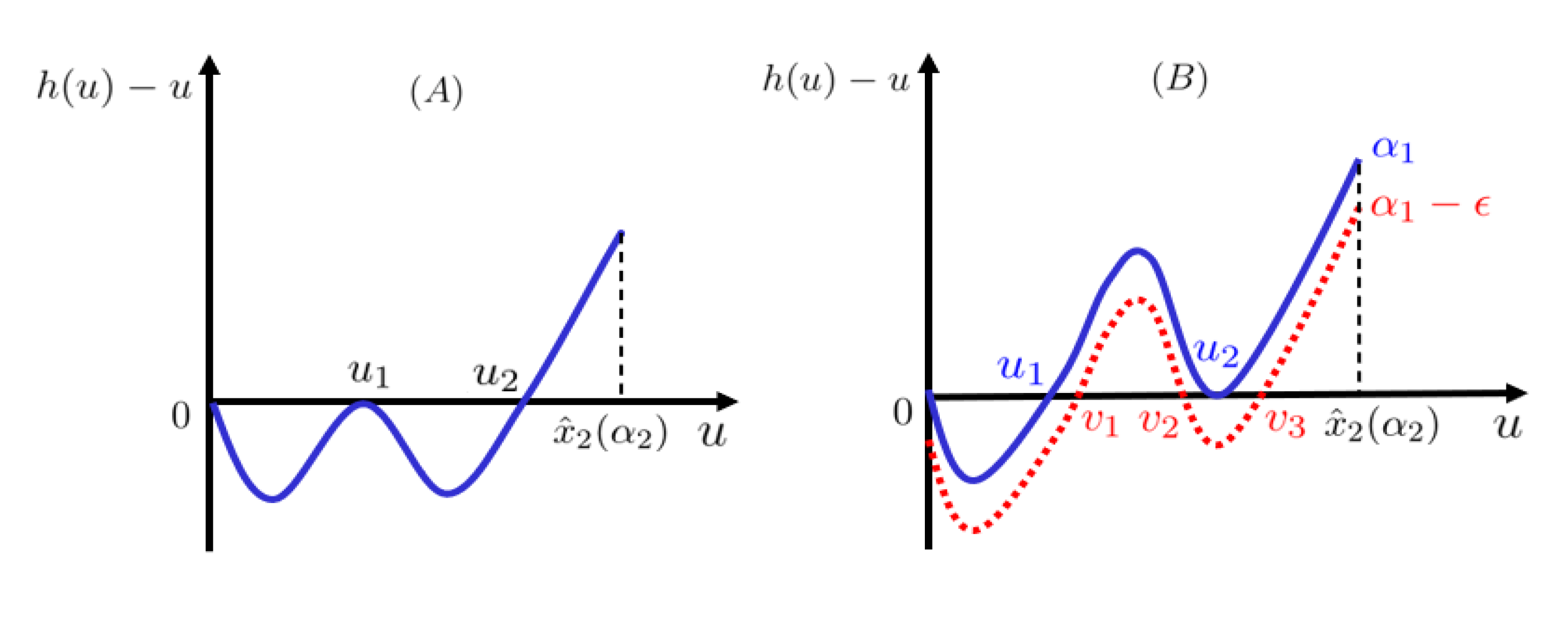
We assume that models (4) and (5) have another nontrivial T-periodic solution initiated from $u_2\in (u_1,\widehat{x}\left({\alpha }_2\right))$ by contradiction. See Figure 2 for illustration.

Then two cases occur:

$$\left(\mathrm{i}\right)h^{\prime }\left(u_1\right)=1\mathrm{and}{h}^{\prime }\left(u_2\right)\ge 1,\left(\mathrm{ii}\right)h^{\prime }\left(u_1\right)\ge 1\mathrm{and}{h}^{\prime }\left(u_2\right)=1.$$

(31)

On case (i), we have $h^{\prime }\left(u_1\right)=1$, $h^{\prime }\left(u_2\right)\ge 1$, which lead to $g\left(u_1\right)=0$ and $g\left(u_2\right)\ge 0$, this contradicts the conclusion in Lemma 5. In case (ii), we get $h^{\prime }\left(u_1\right)\ge 1$, $h^{\prime }\left(u_2\right)=1$, which goes well with the monotonicity of function $y=g\left(u\right)$. To achieve a contradiction, we rewrite:

$$h\left(u\right)=h(u,{\alpha }_1),\overline{h}\left(u\right)=\overline{h}(u,{\alpha }_1),\mathrm{and}g\left(u\right)=g(u,{\alpha }_1)$$

to consider the monotonicity of these functions in ${\alpha }_1$.

From (21), we arrive at:

$$\frac{\partial \overline{h}(u,{\alpha }_1)}{\partial {\alpha }_1}=\frac{(1-s_f){(1-u)}^{2}u}{Q_1^2\left(u\right)}.$$

(32)

Then, from (22) and (32), we have:

$$\begin{array}{cc}\hfill \frac{\partial h(u,{\alpha }_1)}{\partial {\alpha }_1}=& \frac{\partial }{\partial \overline{h}(u,{\alpha }_1)}\left(\frac{P_2\left(\overline{h}(u,{\alpha }_1)\right)}{Q_2\left(\overline{h}(u,{\alpha }_1)\right)}\right)·\frac{\partial \overline{h}(u,{\alpha }_1)}{\partial {\alpha }_1}\hfill \\ \hfill =& \frac{{(1-s_f)}^2{(1-u)}^2{(1-\overline{h}(u,{\alpha }_1))}^2\overline{h}(u,{\alpha }_1)u}{Q_1^2\left(u\right)Q_2^2\left(\overline{h}(u,{\alpha }_1)\right)}\hfill \\ \hfill >& 0,\hfill \end{array}$$

which implies that $h(u,{\alpha }_1)$ is strictly increasing in ${\alpha }_1\ge 0$. Hence, the function $h(u,{\alpha }_1)-u$ is also strictly increasing in ${\alpha }_1$.

Finding $\epsilon$ small enough, such that ${\alpha }_1-\epsilon >{\alpha }_2$, from the monotonicity of $h(u,{\alpha }_1)-u$ respect of ${\alpha }_1$, we observe that the curve $h(u,{\alpha }_1-\epsilon )$ totally lies below $h(u,{\alpha }_1)-u$ except at $u=0$, which admits three zeros, $u_1<v_1<v_2<u_2<v_3$ with:

$$\frac{\partial h(u,{\alpha }_1-\epsilon )}{\partial u}{|}_{u=v_1}\ge 1,\frac{\partial h(u,{\alpha }_1-\epsilon )}{\partial u}{|}_{u=v_2}\le 1,\frac{\partial h(u,{\alpha }_1-\epsilon )}{\partial u}{|}_{u=v_3}\ge 1.$$

See Figure 2B for illustration. This implies that $g(v_1,{\alpha }_1-\epsilon )\ge 0,g(v_2,{\alpha }_1-\epsilon )\le 0$ and $g(v_3,{\alpha }_1-\epsilon )\ge 0$, which contradicts the monotonicity of $g(u,{\alpha }_1-\epsilon )$ in u, proving the Theorem. □

4. Discussion

The endosymbiotic bacterium Wolbachia was first identified in 1924, which naturally infects 60% of insect species. In mosquitoes, Wolbachia often induces CI which results in early embryonic death when Wolbachia-infected males mate with uninfected females. However, Wolbachia-infected females produce viable and infected embryos owing to the mechanism of maternal transmission, irrelevant of the paternal infection status. The CI mechanism and maternal transmission of Wolbachia bring a reproductive advantage of infected mosquitoes over uninfected ones. Regarding Wolbachia release, the infected males can sterilize uninfected females through CI, and the release of infected females can increase Wolbachia infection frequency in mosquito populations through maternal transmission. To date, two release strategies have been applied in field trials: population suppression by only releasing infected males to sterilize wild females, and population replacement by releasing both infected females and males so that wild mosquitoes are replaced by infected ones.

The field trials of both population suppression and population replacement have been implemented in several countries, including Australia, Brazil, and China, which shows that Wolbachia release is becoming a safe and sustainable approach to controlling mosquito populations and mosquito-borne disease transmission. Particularly, since March 2015, by combining the incompatible and sterile insect techniques (IIT-SIT), Wolbachia-infected male mosquitoes have been released on two isolated islands in south of Guangzhou city. The implementation of IIT-SIT in 2016 and 2017 eradicated more than 95% of wild-type Aedes albopictus populations [25]. As collaborates, we took charge in mathematical modeling in this project, and our discrete mathematical model driven by semi-field cage experiments “accurately described and predicted target population dynamics in the semi-field cage experiments, and supported the notion that a 5:1 over-flooding ratio of HC (the name of the Wolbachia strain) to wild-type males is sufficient for effective population suppression and/or elimination”.

The notion of supplemental releases is motivated by the implementation of incompatible and sterile insect techniques combined to eliminate mosquitoes in Guangzhou, Guangdong China since 2015 [25], where supplementary releases are frequently carried out to guarantee the population suppression. Very recently, we summarized works on Wolbachia spread dynamics since 1959 in [26] and proposed some open questions on the periodic and impulsive release strategies. We took our first try in [27] to answer one of them. This is a continual study aiming to count the exact numbers of nontrivial periodic solutions to the discrete switching model, which is a challenging task to achieve due to the lack of effective methods.

In [17,18,19], the authors developed mosquito population suppression models by switching to ordinary differential equation (ODE) models in each release waiting period T. The global dynamics of these models were elegantly described by using the corresponding Pioncaré maps $h\left(u\right)$, where u is the initial point. By solving the initial value problems in the first T-periodic interval $[0,T)$, the explicit expression of $h\left(u\right)$ was obtained, and then the existence, and uniqueness of the periodic solutions to the ODE models was equivalent to the existence and uniqueness of the fixed points to the map $h\left(u\right)$. Particularly, at $u\in \mathsf{\Gamma }=\left\{u\right|h\left(u\right)=u\}$, $h^{\prime }\left(u\right)$ can also be explicitly expressed in u, which is a key step to showing the uniqueness of the periodic solutions to the ODE models.

Following this procedure, we obtained sufficient conditions to guarantee that the models (4) and (5) have at least one nontrivial periodic solution in Theorem 2. However, this method of proving the uniqueness does not work for the discrete models developed in this paper except for the case $N=1$ and $T=2$ under which the comparison between $h^{\prime }\left(u\right)$ and 1 can be translated to the comparison between a quartic polynomial $g\left(u\right)$ and 0. By developing the qualitative property of $g\left(u\right)$, sufficient conditions to guarantee the existence and uniqueness of the discrete switching model were obtained in Theorem 3. Unfortunately, for the general N and T, as shown in (7), the Poincaré map $h\left(u\right)$ is a composite function whose explicit expression is absent. Furthermore, when calculating $h^{\prime }\left(u\right)$ for the general N and T, we find that it is an impossible mission to get a similar expression as shown in (19). This drives us to seek new methods to treat the general cases in our future research.

References

- Zeng, Z.; Zhan, J.; Chen, L.; Chen, H.; Cheng, S. Global, regional, and national dengue burden from 1990 to 2017: A systematic analysis based on the global burden of disease study 2017. EclinicalMedicine 2021, 32, 100712. [Google Scholar] [CrossRef] [PubMed]
- Arkin, F. Dengue researcher faces charges in vaccine fiasco. Science 2019, 364, 320. [Google Scholar] [CrossRef] [PubMed]
- Bardina, S.V.; Bunduc, P.; Tripathi, S.; Duehr, J. Enhancement of Zika virus pathogenesis by preexisting antiflavivirus immunity. Science 2017, 356, 175–180. [Google Scholar] [CrossRef] [PubMed] [Green Version]
- Wang, Y.; Liu, X.; Li, C.; Su, T. A survey of insecticide resistance in Aedes albopictus (Diptera: Culicidae) during a 2014 dengue fever outbreak in Guangzhou, China. J. Econ. Entomol. 2017, 110, 239–244. [Google Scholar]
- Xi, Z.; Dean, J.L.; Khoo, C.C. Generation of a novel Wolbachia infection in Aedes albopictus (Asian tiger mosquito) via embryonic microinjection. Insect Biochem. Mol. Biol. 2005, 35, 903–910. [Google Scholar] [CrossRef] [PubMed] [Green Version]
- Xi, Z.; Khoo, C.C.; Dobson, S.I. Wolbachia establishment and invasion in an Aedes aegypti laboratory population. Science 2005, 310, 326–328. [Google Scholar] [CrossRef] [PubMed] [Green Version]
- Bian, G.; Joshi, D.; Dong, Y.; Lu, P. Wolbachia Invades Anopheles stephensi populations and induces refractoriness to Plasmodium Infection. Science 2013, 340, 748–751. [Google Scholar] [CrossRef] [PubMed]
- Mcmeniman, C.J.; Lane, R.V.; Cass, B.N.; O’Neill, S.L. Stable introduction of a life-shortening Wolbachia Infection into the Mosquito Aedes aegypi. Science 2009, 323, 141–144. [Google Scholar] [CrossRef] [PubMed] [Green Version]
- Walker, T.; Johnson, P.H.; Moreira, L.A.; Leong, Y.S. The wMel Wolbachia strain blocks dengue and invades caged Aedes aegypti populations. Nature 2011, 476, 450–453. [Google Scholar] [CrossRef]
- Hoffmann, A.A.; Montgomery, B.L.; Popovici, J.; Greenfield, M. Successful establishment of Wolbachia in Aedes populations to suppress dengue transmission. Nature 2011, 476, 454–457. [Google Scholar] [CrossRef]
- Caspari, E.; Watson, G.S. On the evolutionary importance of cytoplasmic sterility in mosquitoes. Evolution 1959, 13, 568–570. [Google Scholar] [CrossRef]
- Fine, P.E.M. Vectors and vertical transmission: An epidemiologic perspective. Ann. N. Y. Acad. Sci. 1975, 266, 173–194. [Google Scholar] [CrossRef] [PubMed]
- Fine, P.E.M. On the dynamics of symbiote-dependent cytoplasmic incompatibility in Culicine mosquitoes. J. Invertebr. Pathol. 1978, 31, 10–18. [Google Scholar] [CrossRef]
- Turelli, M.; Hoffmann, A.A. Rapid spread of an inherited incompatibility factor in California Drosophila. Nature 1991, 353, 440–442. [Google Scholar] [CrossRef] [PubMed]
- Turelli, M. Evolution of incompatibility-inducing microbes and their hosts. Evolution 1994, 48, 1500–1513. [Google Scholar] [PubMed]
- Turelli, M. Cytoplasmic incompatibility in populations with overlapping generations. Evolution 2010, 64, 232–241. [Google Scholar] [CrossRef]
- Yu, J. Existence and stability of a unique and exact two periodic orbits for an interactive wild and sterile mosquito model. J. Differ. Equ. 2020, 269, 10395–10415. [Google Scholar] [CrossRef]
- Yu, J.; Li, J. Global asymptotic stability in an interactive wild and sterile mosquito model. J. Differ. Equ. 2020, 269, 6193–6215. [Google Scholar] [CrossRef]
- Zheng, B.; Yu, J.; Li, J. Modeling and analysis of the implementation of the Wolbachia incompatible and sterile insect technique for mosquito population suppression. SIAM J. Appl. Math. 2021, 81, 718–740. [Google Scholar] [CrossRef]
- Shi, Y.; Zheng, B. Discrete dynamical models on Wolbachia infection frequency in mosquito populations with biased release ratios. J. Biol. Dyn. 2021. [Google Scholar] [CrossRef]
- Zheng, B.; Tang, M.; Yu, J. Modeling Wolbachia spread in mosquitoes through delay differential equations. SIAM J. Appl. Math. 2014, 74, 743–770. [Google Scholar] [CrossRef]
- Zheng, B.; Tang, M.; Yu, J.; Qiu, J. Wolbachia spreading dynamics in mosquitoes with imperfect maternal transmission. J. Math. Biol. 2018, 76, 235–263. [Google Scholar] [CrossRef]
- Zheng, B.; Yu, J.; Xi, Z.; Tang, M. The annual abundance of dengue and Zika vector Aedes albopictus and its stubbornness to suppression. Ecol. Model. 2018, 387, 38–48. [Google Scholar] [CrossRef]
- Yu, J.; Zheng, B. Modeling Wolbachia infection in mosquito population via discrete dynamical models. J. Differ. Equ. Appl. 2019, 25, 1549–1567. [Google Scholar] [CrossRef]
- Zheng, X.; Zhang, D.; Li, Y.; Yang, C.; Wu, Y.; Liang, X.; Pan, X.; Hu, L.; Sun, Q.; Wang, X.; et al. Incompatible and sterile insect techniques combined eliminate mosquitoes. Nature 2019, 572, 56–61. [Google Scholar] [CrossRef]
- Zheng, B.; Li, J.; Yu, J. One discrete dynamical model on Wolbachia infection frequency in mosquito populations. Sci. China Math. 2021. [Google Scholar] [CrossRef]
- Zheng, B.; Yu, J. Existence and uniqueness of periodic orbits in a discrete model on Wolbachia Infection Frequency. Adv. Nonlinear Anal. 2021, 11, 212–224. [Google Scholar] [CrossRef]
Figure 1.
Numerical simulations displaying the dynamics of against u. Panel (A) is for the case with the release ratios and satisfying (i) in (17). And the release ratios in panel (B) meet (ii) in (17).
Publisher’s Note: MDPI stays neutral with regard to jurisdictional claims in published maps and institutional affiliations. |
© 2021 by the authors. Licensee MDPI, Basel, Switzerland. This article is an open access article distributed under the terms and conditions of the Creative Commons Attribution (CC BY) license (https://creativecommons.org/licenses/by/4.0/).
Share and Cite
MDPI and ACS Style
Chang, L.; Shi, Y.; Zheng, B. Existence and Uniqueness of Nontrivial Periodic Solutions to a Discrete Switching Model. Mathematics 2021, 9, 2377. https://0-doi-org.brum.beds.ac.uk/10.3390/math9192377
AMA Style
Chang L, Shi Y, Zheng B. Existence and Uniqueness of Nontrivial Periodic Solutions to a Discrete Switching Model. Mathematics. 2021; 9(19):2377. https://0-doi-org.brum.beds.ac.uk/10.3390/math9192377
Chicago/Turabian StyleChang, Lijie, Yantao Shi, and Bo Zheng. 2021. "Existence and Uniqueness of Nontrivial Periodic Solutions to a Discrete Switching Model" Mathematics 9, no. 19: 2377. https://0-doi-org.brum.beds.ac.uk/10.3390/math9192377
Note that from the first issue of 2016, this journal uses article numbers instead of page numbers. See further details here.