Retrial Queues with Unreliable Servers and Delayed Feedback

Abstract

In this paper, models of unreliable multi-server retrial queues with delayed feedback are examined. The Bernoulli retrial is allowed upon the arrival of both primary (from outside) and feedback customers (from orbit), as well as the Bernoulli feedback that may occur after each service in this system. Servers can break down both during the service of customers and when they are idle. If a server breaks down during the service of a customer, then the interrupted customer, in accordance with the Bernoulli scheme, decides either to leave the system or join a common orbit of retrial and feedback customers. An approximate method, based on the space merging approach of three-dimensional Markov chains, is proposed for the calculation of the steady-state probabilities, as well as performance measures of the system. The results of the numerical experiments are demonstrated.

1. Introduction

The theory of retrial queue (RQ) is widely implemented for modeling the functioning of real-world systems. State of the art theory of RQ might be found in the recent review [1]. The general property of RQ is the following: if upon arrival of a primary customer, all servers of the system and/or waiting rooms are full, then a primary customer can join the group of customers that are waiting for the service outside of the system. This virtual waiting room is called orbit for retrial customers. As a rule, in the classical theory of RQ, it is assumed that the system has no information about the number of retrial customers in the orbit, and retrial customers generate their requests independently of each other.

In classical RQ, both primary and retrial customers leave the system after getting the required service. However, in many cases, some customers require an arbitrary number of optional services aside from the essential services. In such systems, some customers provide feedback to the system for optional service. These customers are referred to as feedback customers. Note that a customer can provide feedback either instantaneously after leaving the server or after some delay. Retrial queues with delayed feedback (RQwDFB) are very useful tools for modeling stochastic processes arising in communication networks, call centers, queueing-inventory systems, etc. This paper analyzes the steady-state behavior of an unreliable multi-server retrial queueing system, first with essential services and then with an arbitrary number of optional services.

2. Related Work

To see the importance of RQwDFB, the interested reader is referred to papers [2,3,4,5,6,7,8,9], and their references lists.

In the above-mentioned papers, the models of RQwDFB with reliable servers are investigated. However, in practice, the servers of the systems are subject to random breakdowns; therefore, it is necessary to study the model of RQwDFB with unreliable servers. Models of RQwDFB with unreliable servers have been investigated in a small number of papers in the last few years, see [10,11,12,13,14,15,16,17]. In the indicated papers, single-server models are considered.

Note that the models of unreliable multi-server RQ without feedback phenomena were investigated using the Space Merging Method (SMM) in [18,19,20]. Similar models have been investigated in [21] using an asymptotic approach. In indicated papers, it is assumed that the parameters of the Bernoulli trial that determine decisions for primary customers to join the orbit or leave the system over the absence of free servers are state-independent. Further, parameters of the Bernoulli trial that determine decisions for customers to enter the orbit that are preempted due to a server failure or abandoning the service are state-independent. Moreover, in known models, as a rule, it is assumed that both active and idle breakdowns occur at the same rate. These assumptions essentially restrict the application areas of the obtained results.

To our best knowledge, models of unreliable multi-server RQwDFB have not been studied. In this paper, models of unreliable multi-server RQwDFB are investigated under more general assumptions using SMM. The method is the same; however, the system is different, and the parameters of the Bernoulli trial that determine appropriate decisions in the system are state-dependent for the model with a finite orbit size. The last assumption leads to more complex equations and solutions. For historical justice, it is necessary to note that the SMM was initially used to calculate the steady-state probabilities of the two-dimensional Markov chain (2D MC) in [22]. In the last decade, [23,24,25] have developed similar algorithms to study 2D MC in various areas of application. In all papers, the authors note the high efficiency of SMM (both in the sense of accuracy and complexity) in comparison with other numerical methods.

This paper is structured as follows: Basic mathematical models of the investigated multi-server unreliable RQwDFB are described in Section 3. The generator matrix of the appropriate 2D MC that represents the mathematical model of the system with a finite orbit size is created in Section 4. Here, the balance equations method of calculating its steady-state probabilities is indicated, and explicit formulas for the performance measures of the investigated system are developed, as well. In Section 5, the approximate SMM for calculating steady-state probabilities and performance measures of the system with an infinite orbit size is proposed. The results of numerical experiments that show the behavior of performance measures versus system parameters are demonstrated in Section 6. Conclusions are given in Section 7.

3. Model Description

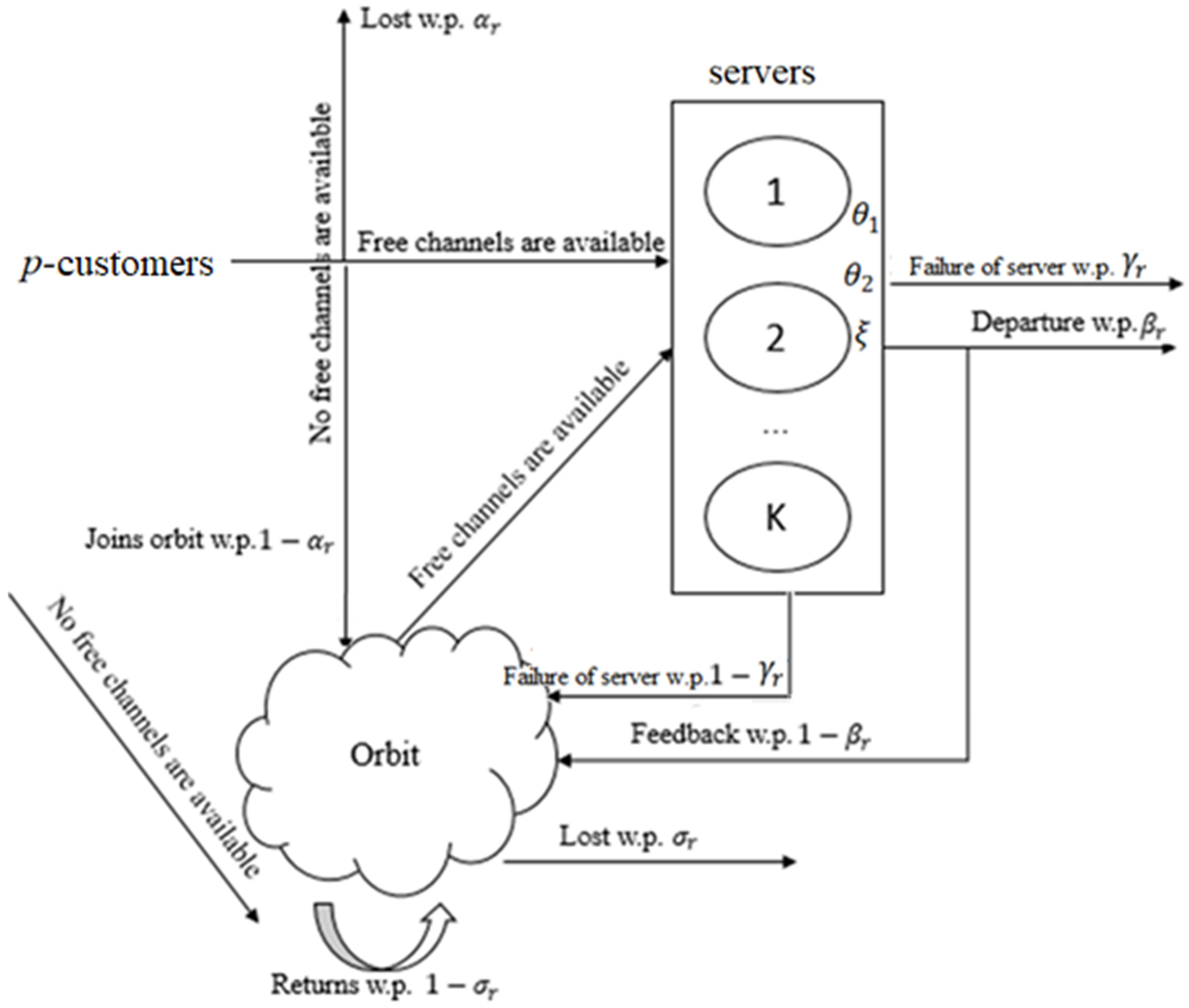
A pictorial representation of the investigated RQwDFB with unreliable servers is shown in Figure 1.

First, consider the model with a finite capacity of orbit for retrial customers, i.e., assume that the maximal size of orbit is equal to $R, R<\infty$. The system contains $K>1$ identical and unreliable servers. It is assumed that servers can independently break down in both busy and idle modes. The failure rate of servers is different in their various statuses, i.e., failures of servers in both busy and idle statuses occur via two independent Poisson processes with rates of ${\theta }_1$ and ${\theta }_2$, respectively. Each server also has its own repairman and the repair times for servers are exponentially distributed with the common rate $\xi$. If the failure of a server occurs during the busy status (active breakdown), then a customer that is preempted due to a server failure either leaves the system (i.e., is lost) with a probability (w.p.) ${\gamma }_r$ or enters the retrial orbit w.p. $1-{\gamma }_r$, provided that there are $r$ customers in the orbit, $r=0, 1, \dots , R-1 ; {\gamma }_R=1$.

Primary customers (p-customers) form Poisson flow with rate $\lambda$. An incoming p-customer is accepted for service if at this moment the total number of busy and failed servers is less than $K$; otherwise, they either leave the system w.p. ${\alpha }_r$ or go to orbit w.p. $1-{\alpha }_r$ provided that there are $r$ customers in the orbit, $r=0, 1, \dots , R-1 ; {\alpha }_R=1$.

Sojourn times of retrial customers (r-customers) in the orbit are exponentially distributed with a mean ${\eta }^{-1}$ and here a classical retrial scheme is considered, i.e., if there are $r$ customers in the orbit, then the arrival intensity of r-customers is $r\eta$ (linear retrial rate). If upon the arrival of r-customer there is no free and serviceable server, then they either leave the orbit (i.e., are lost) w.p. σ_r or return to the orbit w.p. 1 − σ_r provided that there are r customers in the orbit, $r=1, \dots , R$.

After the completion of the service process, the customer either leaves the system forever w.p. ${\beta }_r$ or goes to the orbit for repeated service w.p. $1-{\beta }_r$ provided that there are r customers in the orbit, $r=0, 1, \dots , R-1 ; {\beta }_R=1$. customers in the orbit, r = 0, 1, …, R − 1; β = 1. Customers who require re-service are called feedback customers (f-customers). For simplicity, in the orbit, both kinds of customers (i.e., r-customers and f-customers) are treated as the same and they are referred to as r-customers. Here, multiple re-servicing processes (feedbacks) are allowed.

For the model with an infinite orbit capacity for retrial and feedback customers, i.e., when $R=\infty$, we assume that ${\alpha }_r<1 , {\beta }_r<1 , {\gamma }_r<1$ for any value of $r$.

The service times for all kinds of customers (p-, r-, and f-customers) are assumed to be exponentially distributed with a common mean ${\mu }^{-1}$.

All times involved in the model, as well as the arrival of p-customers from the outside, the arrival of r-customers from the orbit, and the service of customers, are mutually independent of each other.

Our goal is to determine the stationary distribution of the given system, as well as to calculate its performance measures: loss probabilities of both p-customers and r-customers, the average number of both failed and busy servers, and the average number of r-customers in the orbit.

4. Balance Equations Method for the Model with a Finite Orbit Size

The state of the system is defined by a three-dimensional vector $(b, f, r)$, where $b$ is the number of busy servers, $f$ is the number of failure servers, and $r$ is the number of r-customers in the orbit. In other words, the mathematical model of the given system is 3D MC with the following state space (SS):

$$S={\displaystyle \underset{r=0}{\overset{R}{\cup }}{S}_r} , S_r{\displaystyle \cap S_{r^{\prime }}}=\varnothing , r\ne r^{\prime } ,$$

(1)

where $S_r=\left\{\left(b,f,r\right) : 0\le b+f\le K\right\} , r=0, 1 ,\dots , R$.

It is clear that in the state $(b, f, r)\in S$, the number of idle and serviceable servers is equal to $K-b-f .$ From (1), we conclude that the SS of the investigated 3D MC geometrically represents a prism with height $R$. Consider the problem of constructing the generator of the indicated 3D MC.

Let us fix the value of $r$ and first consider determining transition intensities between the states within a subset (level), $S_r$. In order to be short, a transition from state $(b, f, r)\in S_r$ to state $(b^{\prime }, f^{\prime }, r^{\prime })\in S_{r^{\prime }}$ with intensity $a$ is denoted by $\left(b,f,r\right)\stackrel{a}{\to }\left(b^{\prime },f^{\prime },r^{\prime }\right) .$ Let the initial state be $(b, f, r)\in S$. As a result of analyzing possible transitions, we have the following relations:

• $(b, f,r)\stackrel{\lambda }{\to }\left(b+1,f,r\right)$ is carried out upon receipt of the p-customer if $b+f<K$;
• $(b, f, r)\stackrel{b{\mu }_r}{\to }\left(b-1,f,r\right)$ is carried out upon departure of the customer from the system or their loss due to a server’s active breakdown, where ${\mu }_r=\mu {\beta }_r+{\theta }_1{\gamma }_r$;
• $(b, f, r)\stackrel{\left(K-b-f\right){\theta }_2}{\to }\left(b,f+1,r\right)$ is carried out when the failure of a server occurs in its idle status;
• $(b, f, r)\stackrel{f\xi }{\to }\left(b,f-1,r\right)$ is carried out when the repair of a failed server is completed;

Now consider determining the transition intensities between the states of the various subsets (levels). Note that only transitions between states of neighboring levels are allowed. For such kinds of transitions, we have the following relations:

• $(b, f,r)\stackrel{\lambda \left(1-{\alpha }_r\right)}{\to }\left(b,f,r+1\right)$ is carried out upon the joining of the arrived p-customer to orbit when $b+f=K$ and $r<R$;
• $(b, f, r)\stackrel{b\mu \left(1-{\beta }_r\right)}{\to }\left(b-1,f,r+1\right)$ is carried out when the serviced customer feedbacks to the orbit when $r<R$;
• $(b, f, r)\stackrel{f{\theta }_1\left(1-{\gamma }_r\right)}{\to }\left(b,f+1,r+1\right)$ is carried out when the customer goes to orbit due to a server’s active breakdown when $r<R$;
• $(b, f, r)\stackrel{r\eta }{\to }\left(b+1,f,r-1\right)$ is carried out upon receipt of the r-customer if $b+f<K$ when $r>0$;
• $(b, f, r)\stackrel{r\eta {\sigma }_r}{\to }\left(b,f,r-1\right)$ is carried out when an arrived r-customer is lost, if $b+f=K$, when $r>0$.

The transition intensity from state $(b, f, r)$ to state $(b^{\prime }, f^{\prime }, r^{\prime })$ is denoted by $q((b,f,r),(b^{\prime },f^{\prime },r^{\prime }))$. From the above relations, we conclude that the positive elements of the generator of the investigated 3D MCs are determined as follows:

$$q\left(\left(b,f,r\right),\left(b^{\prime }, f^{\prime },r^{\prime }\right)\right)=\{\begin{array}{ll}\lambda \hfill & \mathrm{if} b+f<K,\left(b^{\prime },f^{\prime },r^{\prime }\right)=\left(b+1,f,r\right)\hfill \\ b{\mu }_r\hfill & \mathrm{if} \left(b^{\prime },f^{\prime },r^{\prime }\right)=\left(b-1,f,r\right)\hfill \\ \left(K-b-f\right){\theta }_2\hfill & \mathrm{if} \left(b^{\prime },f^{\prime },r^{\prime }\right)=\left(b,f+1,r\right)\hfill \\ f\xi \hfill & \mathrm{if} \left(b^{\prime },f^{\prime },r^{\prime }\right)=\left(b,f-1,r\right)\hfill \\ \lambda \left(1-{\alpha }_r\right)\hfill & \mathrm{if} r<R, b+f<K,\left(b^{\prime },f^{\prime },r^{\prime }\right)=\left(b,f,r+1\right)\hfill \\ b\mu \left(1-{\beta }_r\right)\hfill & \mathrm{if} r<R, \left(b^{\prime },f^{\prime },r^{\prime }\right)=\left(b-1,f,r+1\right)\hfill \\ f{\theta }_1\left(1-{\gamma }_r\right)\hfill & \mathrm{if} r<R, \left(b^{\prime },f^{\prime },r^{\prime }\right)=\left(b,f+1,r+1\right)\hfill \\ r\eta \hfill & \mathrm{if} b+f<K,r>0,\left(b^{\prime },f^{\prime },r^{\prime }\right)=\left(b+1,f,r-1\right)\hfill \\ r\eta {\sigma }_r\hfill & \mathrm{if} b+f=K,r>0,\left(b^{\prime },f^{\prime },r^{\prime }\right)=\left(b,f,r-1\right) .\hfill \end{array}$$

(2)

Hereinafter, the equality of vectors means that their corresponding components are equal to one another.

From the relations (2), we conclude that states of constructed finite 3D MCs are communicated with each other, i.e., a stationary mode exists in this system. Let $p\left(b,f,r\right)$ denote the stationary probability of the state $\left(b,f,r\right)\in S$. These probabilities can be found using the following balance equations:

$${\displaystyle \sum _{\left(b^{\prime },f^{\prime },r^{\prime }\right)\in S_{\left(b,f,r\right)}^{+}}q\left(\left(b,f,r\right) ,\left(b^{\prime },f^{\prime },r^{\prime }\right)\right)}p\left(b,f,r\right)={\displaystyle \sum _{\left(b^{\prime },f^{\prime },r^{\prime }\right)\in S_{\left(b,f,r\right)}^{-}}q\left(\left(b^{\prime },f^{\prime },r^{\prime }\right) ,\left(b,f,r\right)\right)p\left(b^{\prime },f^{\prime },r^{\prime }\right)} ;$$

(3)

$${\displaystyle \sum _{\left(b,f,r\right)\in S}p\left(b,f,r\right)}=1 ,$$

(4)

where $S_{\left(b,f,r\right)}^{+}$ is the set of those states of $S$, which can be reached from the state $\left(b,f,r\right)$ in one step, and $S_{\left(b,f,r\right)}^{-}$ is the set of those states of $S$, from which one can get to the state $\left(b,f,r\right)$ in one step. Note that the sets $S_{\left(b,f,r\right)}^{+}$ and $S_{\left(b,f,r\right)}^{-}$ are determined from the relations (2).

The dimension of the balance Equations (3) and (4) is equal to $\left(K+1\right)\left(K+2\right)\left(R+1\right)/2$. Modern software packages allow the linear equations of arbitrary (finite) dimensions to be solved.

The desired performance measures are calculated via steady-state probabilities. The average number of busy $\left(NB{S}_{av}\right)$ and failed servers $\left(NF{S}_{av}\right)$, as well as the average number of r-customers in the orbit $\left(NC{O}_{av}\right)$, are calculated as the mathematical expectations of the corresponding random variables, i.e.,

$$NB{S}_{av}={\displaystyle \sum _{b=1}^{K}b}{\displaystyle \sum _{\left(b,f,r\right)\in S}p\left(b,f,r\right)} ;$$

(5)

$$NB{S}_{av}={\displaystyle \sum _{f=1}^{K}f}{\displaystyle \sum _{\left(b,f,r\right)\in S}p\left(b,f,r\right)} ;$$

(6)

$$NC{O}_{av}={\displaystyle \sum _{r=1}^{R}r}{\displaystyle \sum _{\left(b,f,r\right)\in S}p\left(b,f,r\right)} .$$

(7)

The loss probabilities of p-customers $\left(P_p\right)$ and r-customers $\left(P_r\right)$ are calculated as

$$P_p={\displaystyle \sum _{r=0}^R{\alpha }_r}{\displaystyle \sum _{\left(b,f,r\right)\in S}p\left(b,f,r\right)\delta \left(b+f,K\right)} ;$$

(8)

$$P_r={\displaystyle \sum _{r=1}^R{\sigma }_r}{\displaystyle \sum _{\left(b,f,r\right)\in S}p\left(b,f,r\right)\delta \left(b+f,K\right)} .$$

(9)

Hereinafter $\delta \left(i,j\right)$ are Kronecker’s delta.

5. The Space Merging Method for the Model with an Infinite Orbit Size

Methodological difficulties occur in solving the investigated problem for the model with an infinite orbit size, i.e., when $R=\infty$. Now consider this problem for the case where the indicated above probabilities, ${\alpha }_r, {\beta }_r, {\gamma }_r, {\sigma }_r$, are state-independent, i.e., assume that ${\alpha }_r=\alpha , {\beta }_r=\beta , {\gamma }_r=\gamma , {\sigma }_r=\sigma$.

The mathematical model of the given system is 3D MC with the following state space (SS):

$$E={\displaystyle \underset{r=0}{\overset{\infty }{\cup }}{E}_r} , E_r{\displaystyle \cap E_{r^{\prime }}}=\varnothing , r\ne r^{\prime } ,$$

(10)

where $E_r=\left\{\left(b,f,r\right) : 0\le b+f\le K\right\} , r=0, 1 ,\dots$

From (10), we conclude that the SS of the investigated 3D MC geometrically represents an infinite prism. The generator of the presently examined infinite 3D MC is determined similarly to (2), wherein the right side condition, $r<R$, should be omitted.

For simplicity, let $p\left(b,f,r\right)$ again denote the stationary probability of the state $\left(b,f,r\right)\in E$. Below, we show that for the case of the linear retrial rate, the stationary mode exists for any positive values of input parameters; however, in the case of the constant retrial rate, the fulfillment of some stability conditions is required.

From the form of the SS (8), we conclude that the constructed 3D MC does not belong to the class of quasi-birth and death (QBD) processes (see [26]). Therefore, unfortunately, to calculate the steady-state probabilities of the investigated 3D MC, we cannot apply well-worked matrix-geometric methods. For this reason, we propose an alternate approach below to solve the indicated problem. The proposed approach is based on the space merging principles of a multi-dimensional MC and it allows for the calculation of steady-state probabilities and performance metrics via explicit formulas. Moreover, the obtained formulas contain quantities that are tabulated, i.e., Erlang’s B-formula as well as the formula for calculating the average number of busy servers in Erlang’s classical model.

It is known that satisfying the following condition is required for the correct application of the SMM: the state space of the system should be decomposed into classes in such a way that the rates of transitions between states within classes are much larger than rates of transitions between states from different classes. The fulfillment of this condition can be ensured at certain ratios between the initial parameters of the system under study. So, suppose that the arrival rate of p-customers is much larger than the arrival rate of r-customers, i.e., $\eta <<\lambda$.

When this assumption is fulfilled, the transitions between the states within classes $E_r$ (see (10)) are much larger than transition classes between the states of different classes. By using this fact, the following merge function in the SS (10) is defined:

$$U_1\left(\left(b,f,r\right)\right)=<r>, \left(b,f,r\right)\in E_r ,$$

(11)

where $<r>$ is the merged state, which includes all micro-states from the class $E_r$, $r=0, 1, \dots$ The set of merged states $<r>$ is denoted by ${\mathsf{\Omega }}_1=\left\{<r> : r=0, 1, \dots \right\}$.

According to hierarchical SMM (see [7,27]), the approximate values of the steady-state probabilities of the initial 3D MC, denoted by $\tilde{p}\left(b, f,r\right)$, are calculated as follows:

$$\tilde{p}\left(b,f,r\right)={\rho }_r\left(b,f\right){\pi }_1\left(<r>\right) ,$$

(12)

where ${\rho }_r\left(b,f\right)$ is the probability of the state, $(b,f,r)$, within a splitting model with SS $E_r$, and ${\pi }_1\left(<r>\right)$ is the probability of the merged state $<r>\in {\mathsf{\Omega }}_1$.

From (12), conclude that to calculate the steady-state probabilities of the initial 3D MC, it is necessary to find the steady-state probabilities, ${\rho }_r\left(b,f\right)$, of the infinite number of 2D MCs with a finite SS as well as the steady-state probabilities, ${\pi }_1\left(<r>\right)$, of one 1D MC with the SS ${\mathsf{\Omega }}_1$.

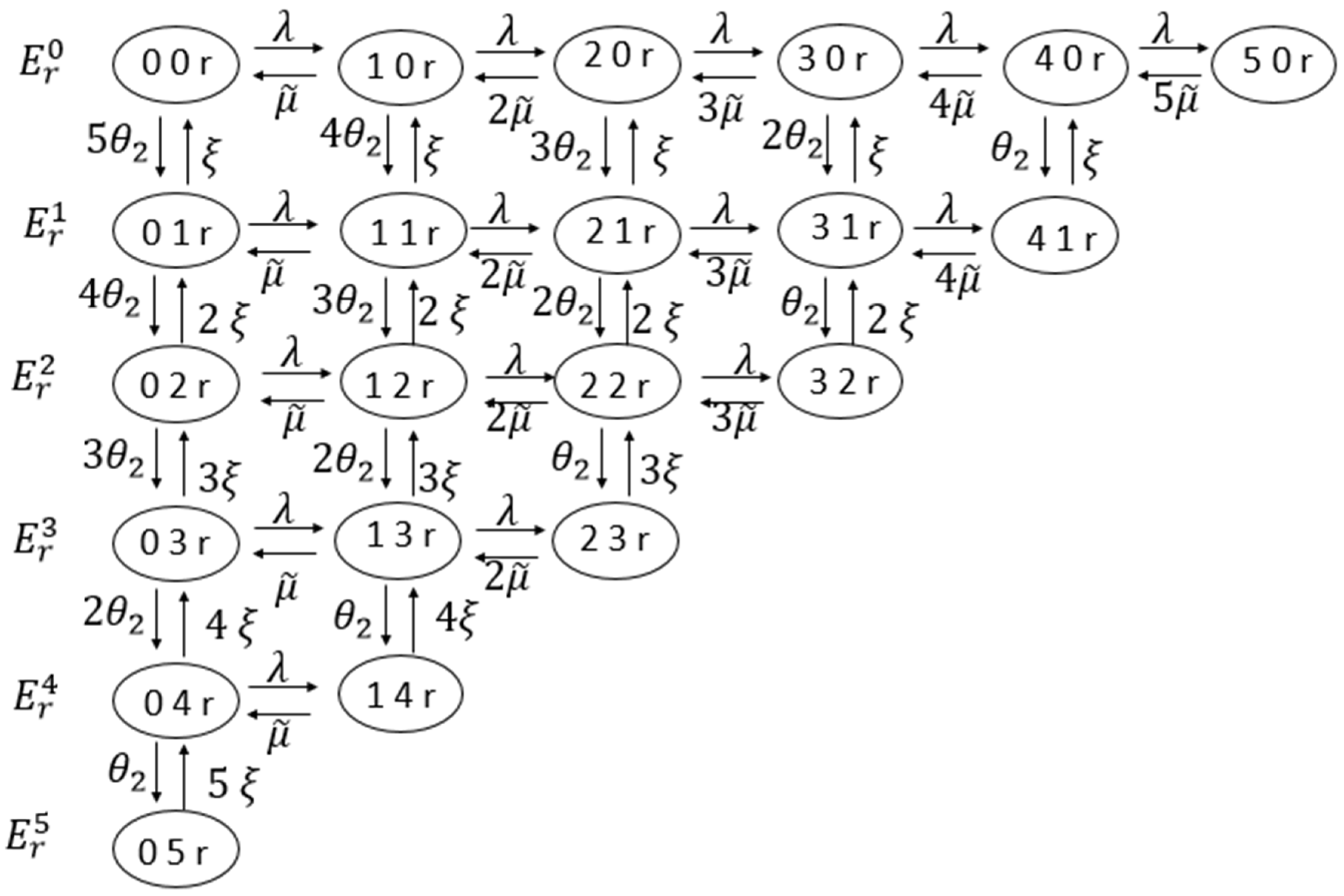
First, consider the calculation of the steady-state probabilities, ${\rho }_r\left(b,f\right)$, of the 2D MCs with the SS $E_r$. The transitions diagram for the splitting model with the SS $E_r$ is shown in Figure 2.

The transition intensity from state $(b, f, r)\in E_r$ to state $(b^{\prime }, f^{\prime }, r)\in E_r$ is denoted by $q_r((b,f,r),(b^{\prime },f^{\prime },r))$. From (2), we conclude that these quantities are determined as follows:

$$q_r((b,f,r),(b^{\prime },f^{\prime },r))=\{\begin{array}{ll}\lambda \hfill & \mathrm{if} b+f<K, \left(b^{\prime },f^{\prime },r\right)=\left(b+1,f,r\right)\hfill \\ b\tilde{\mu }\hfill & \mathrm{if} \left(b^{\prime },f^{\prime },r\right)=\left(b-1,f,r\right)\hfill \\ \left(K-b-f\right){\theta }_2\hfill & \mathrm{if} \left(b^{\prime },f^{\prime },r\right)=\left(b,f+1,r\right)\hfill \\ f\xi \hfill & \mathrm{if} \left(b^{\prime },f^{\prime },r\right)=\left(b,f-1,r\right) ,\hfill \end{array}$$

(13)

where $\tilde{\mu }=\mu \beta +{\theta }_1\gamma$.

From (13), we conclude that $q_r((b,f,r),(b^{\prime },f^{\prime },r))$ are identical for any value of $r$, i.e., the steady-state probabilities, ${\rho }_r\left(b,f\right)$, do not depend on $r$ because, below, we fix the value of $r$ and omit the subscript $r$ in the notation of these quantities.

The calculation of the steady-state probabilities, $\rho \left(b,f\right)$, for a moderately sized SS, $S_r$, might be performed via solving balance equations. However, it is possible to develop explicit formulas for their approximate calculations. For this purpose, the merging procedure (the second level of the hierarchy) is applied to these 2D MCs.

For the correct application of the SMM in the second level, it is assumed that ${\theta }_1>>{\theta }_2$. Note that this assumption is a realistic one since, in real situations, the failure intensity of servers in a busy mode is much higher than for those in an idle mode. Under this assumption, consider the following splitting of $S_r$:

$$E_r={\displaystyle \underset{f=0}{\overset{K}{\cup }}{E}_r^f} , E_r^f{\displaystyle \cap E_r^{f^{\prime }}=\varnothing ,f\ne f^{\prime }} ,$$

(14)

where $E_r^f=\left\{\left(b,f\right)\in E_r: b=0, 1, \dots , K;b+f\le K\right\}, f=0, 1, \dots ,K$.

Similar to (11), based on splitting (14) in the SS, $E_r$, the following merge function is defined:

$$U_2\left(\left(b,f\right)\right)=<<f>> ,\left(b,f\right)\in E_r^f,$$

where $<<f>>$ is a merge state which includes all micro-states from the subclass $E_r^f$. The set of merged states $<<f>>$ is denoted by ${\mathsf{\Omega }}_2=\left\{<<f>> : f=0, 1, \dots , K\right\}$.

In accordance with [7,27], we have:

$$\rho \left(b,f\right)\approx {\rho }_f\left(b\right){\pi }_2\left(<<f>>\right) ,$$

(15)

where ${\rho }_f\left(b\right)$ is the probability of the state $(b,f)$ within the splitting model with space $E_r^f$, and ${\pi }_2\left(<<f>>\right)$ is the probability of the merged state $<<f>>\in {\mathsf{\Omega }}_2$.

In a subclass, $E_r^f, f=0, 1, \dots ,K,$ the second component of the state vector is a constant and equals $f$. Therefore, in a splitting model with space $E_r^f$, each state, $(b,f)$, can be represented simply by the first component, i.e., by $b,b=0, 1, \dots , K-f$.

The transition intensity from state $(b, f)\in E_r^f$ to state $(b^{\prime }, f)\in E_r^f$ is denoted by $q(b,b^{\prime })$. So, from relations (2) we conclude that these quantities are independent of the parameter $r$, and are determined as follows:

$$q\left(b,b^{\prime }\right)=\{\begin{array}{ll}\lambda ,\hfill & \mathrm{if} b^{\prime }=b+1 ,\hfill \\ b\left(\mu \beta +{\theta }_1\gamma \right),\hfill & \mathrm{if} b^{\prime }=b-1 .\hfill \end{array}$$

(16)

From (16), we conclude that the state probabilities, ${\rho }_f\left(b\right)$, of the splitting models with the SS $E_r^f, f=0, 1, \dots ,K-1,$ coincides with the state probabilities of Erlang’s model, M/M/K-f/K-f, with load $\nu =\lambda /\left(\mu \beta +{\theta }_1\gamma \right)$, i.e., the desired probabilities are calculated by well-known Erlang’s formulas:

$${\rho }_f\left(b\right)=\frac{{\nu }^b}{b!}/{\displaystyle \sum _{i=0}^{K-f}\frac{{\nu }^i}{i!}} , b=0, 1 , \dots , K-f .$$

(17)

The splitting model with the SS $E_r^K$ contains only one state $\left(0,K,r\right)$, i.e., for this model, we set ${\rho }_K\left(0\right)=1$.

The transition intensity from merged state $<<f>>\in {\mathsf{\Omega }}_2$ to merged state $<<f^{\prime }>>\in {\mathsf{\Omega }}_2$ is denoted by $q\left(<<f>>,<<f^{\prime }>>\right)$. By using (2) and (17), after certain mathematical transformations, we conclude that the indicated quantities are determined as follows:

$$q\left(<<f>>,<<f^{\prime }>>\right)=\{\begin{array}{ll}{\Lambda }_f,\hfill & \mathrm{if} f^{\prime }=f+1 ,\hfill \\ f\xi ,\hfill & \mathrm{if} f^{\prime }=f-1 ,\hfill \end{array}$$

(18)

where ${\Lambda }_f={\theta }_2{\displaystyle \sum _{i=0}^{K-f-1}{\rho }_f\left(i\right)}\left(K-f-i\right)$.

Therefore, from relations (18), we conclude that the probabilities of merged states are calculated as follows:

$${\pi }_2\left(<<f>>\right)=\frac{1}{f!{\xi }^f}{\displaystyle \prod _{i=0}^{f-1}{\Lambda }_i}{\pi }_2\left(<<0>>\right) , f=1, \dots , K ,$$

(19)

where ${\pi }_2\left(<<0>>\right)$ is found from the normalizing condition, i.e., ${\displaystyle \sum _{f=0}^K{\pi }_2\left(<<f>>\right)}=1$.

Now consider the problem of finding the probabilities of merged states ${\pi }_1\left(<r>\right) , <r>\in {\mathsf{\Omega }}_1 .$ The transition intensity from state $<r>\in {\mathsf{\Omega }}_1$ to state $<r^{\prime }>\in {\mathsf{\Omega }}_1$ is denoted by $q(<r>, <r^{\prime }>)$. By using (2) (for this model), (17), and (19), we conclude that these quantities are calculated as follows:

$$q\left(<r>,<r^{\prime }>\right)=\{\begin{array}{ll}\varpi ,\hfill & \mathrm{if} r^{\prime }=r+1 ,\hfill \\ r\varphi ,\hfill & \mathrm{if} r^{\prime }=r-1 ,\hfill \end{array}$$

(20)

where

$$\begin{array}{l}\varpi =\left(\mu \left(1-\beta \right)+{\theta }_1\left(1-\gamma \right)\right){\displaystyle \sum _{j=0}^{K-1}\underset{B_{av}\left(K-j,\nu \right)}{\underbrace{{\displaystyle \sum _{i=1}^{K-j}i{\rho }_j\left(i\right)}}}{\pi }_2\left(<<j>>\right)+\lambda \left(1-\alpha \right){\displaystyle \sum _{i=0}^K\underset{E_B\left(K-i,\nu \right)}{\underbrace{{\rho }_i\left(K-i\right)}}{\pi }_2\left(<<i>>\right)}}=\\ =\left(\mu \left(1-\beta \right)+{\theta }_1\left(1-\gamma \right)\right){\displaystyle \sum _{j=0}^{K-1}{B}_{av}\left(K-j,\nu \right)}{\pi }_2\left(<<j>>\right)+\lambda \left(1-\alpha \right){\displaystyle \sum _{i=0}^K{E}_B\left(K-i,\nu \right){\pi }_2\left(<<i>>\right)} ;\end{array}$$

$$\begin{array}{l}\varphi =\eta \left(\underset{1-E_B\left(K,\nu \right)}{\underbrace{{\displaystyle \sum _{i=0}^{K-1}{\rho }_0\left(i\right)}}}{\pi }_2\left(<<0>>\right)+\underset{1-E_B\left(K-1,\nu \right)}{\underbrace{{\displaystyle \sum _{i=0}^{K-2}{\rho }_1\left(i\right)}}}{\pi }_2\left(<<1>>\right)+\dots +\underset{1-E_B\left(1,\nu \right)}{\underbrace{{\rho }_{K-1}\left(0\right)}}{\pi }_2\left(<<K-1>>\right)\right)+\\ +\eta \sigma \left(\underset{E_B\left(K,\nu \right)}{\underbrace{{\rho }_0\left(K\right)}}{\pi }_2\left(<<0>>\right)+\underset{E_B\left(K-1,\nu \right)}{\underbrace{{\rho }_1\left(K-1\right)}}{\pi }_2\left(<<1>>\right)+\dots +\underset{E_B\left(0,\nu \right)}{\underbrace{{\rho }_K\left(0\right)}}{\pi }_2\left(<<K>>\right)\right)=\\ =\eta \left({\displaystyle \sum _{i=1}^K\left(1-E_B\left(i,\nu \right)\right){\pi }_2\left(<<K-i>>\right)}+\sigma {\displaystyle \sum _{i=0}^K{E}_B\left(i,\nu \right){\pi }_2\left(<<K-i>>\right)}\right) .\end{array}$$

Hereinafter, $E_B\left(m, \nu \right)$ and $B_{av}\left(m, \nu \right)$ denote Erlang’s B-formula and the average number of busy servers for the M/M/m/m system with a load, $\nu$, respectively, i.e.,

$$E_B\left(m, \nu \right)=\frac{{\nu }^m}{m!}/{\displaystyle \sum _{i=0}^m\frac{{\nu }^i}{i!}} ; E_B\left(0,\nu \right)=1 ;B_{av}\left(m, \nu \right)=\nu \left(1-E_B\left(m, \nu \right)\right) .$$

From relations (20). we conclude that the probabilities of merged states coincide with the probabilities of the states of the model M/M/∞ with the load $\psi =\varpi /\varphi$, i.e.,

$${\pi }_1\left(<r>\right)=\frac{{\psi }^r}{r!}\exp \left(-\psi \right) , r=0, 1, 2, \dots$$

(21)

By using (12), (15), (17), and (21), the approximate values of the steady-state of the initial 3D MC are found. So, for any positive values of the loading parameters in this system, there exists stationary mode, and after some standard mathematical transformations, we obtain the following approximate formulas for calculating the performance measures:

$$P_p\approx \alpha {\displaystyle \sum _{i=0}^K{E}_B\left(i,\nu \right){\pi }_2\left(<<K-i>>\right)} ;$$

(22)

$$P_r\approx \sigma \left(1-e^{-\psi }\right){\displaystyle \sum _{i=0}^K{E}_B\left(i,\nu \right){\pi }_2\left(<<K-i>>\right)} ;$$

(23)

$$NB{S}_{av}\approx {\displaystyle \sum _{i=1}^{K}i{\displaystyle \sum _{j=0}^{K-i}{\rho }_j\left(i\right){\pi }_2\left(<<j>>\right)}} ;$$

(24)

$$NF{S}_{av}\approx {\displaystyle \sum _{i=1}^{K}i{\pi }_2\left(<<i>>\right)} ;$$

(25)

$$NC{O}_{av}\approx \psi$$

(26)

Note. The average number of busy $\left(NB{S}_{av}\right)$ and failed servers $\left(NF{S}_{av}\right)$ (see Formulas (24) and (25)) does not depend on the parameters $\eta$ and $\sigma$. These facts are explained by the accepted assumption that $\eta <<\lambda$, i.e., the impact of the indicated parameters on two performance measures is not essential. Other performance measures depend on all system parameters.

6. Numerical Results

In this section, the qualitative behavior of the performance measures is explored through a few numerical experiments. Due to the size limitations for the present paper, only the results for the model with an infinite orbit size have been considered here.

It can be noticed that the proposed algorithms allowed for a simple investigation of the behavior of the performance measures over any parameter of the model without any computational difficulties. For the sake of brevity, we have omitted the results of numerical experiments that demonstrate the high accuracy of the algorithm developed for the approximate calculation of steady-state probabilities of the system under study (appropriate results might be found in [9]). Moreover, for brevity, we only demonstrate experiments that present the behavior of performance measures with respect to the number of servers over various values of the probabilities $\alpha ,\beta ,\gamma$ and $\sigma$.

For the numerical calculations, the values of the model parameters are selected as follows: $\lambda =5,\mu =3,{\theta }_1=5,{\theta }_2=1,\xi =1,\eta =1 .$ Note that since the performance measures depend on many parameters, the analysis of the numerical experiments indicated below concerns only the selected values of the initial data. However, in some cases, the conclusions are general.

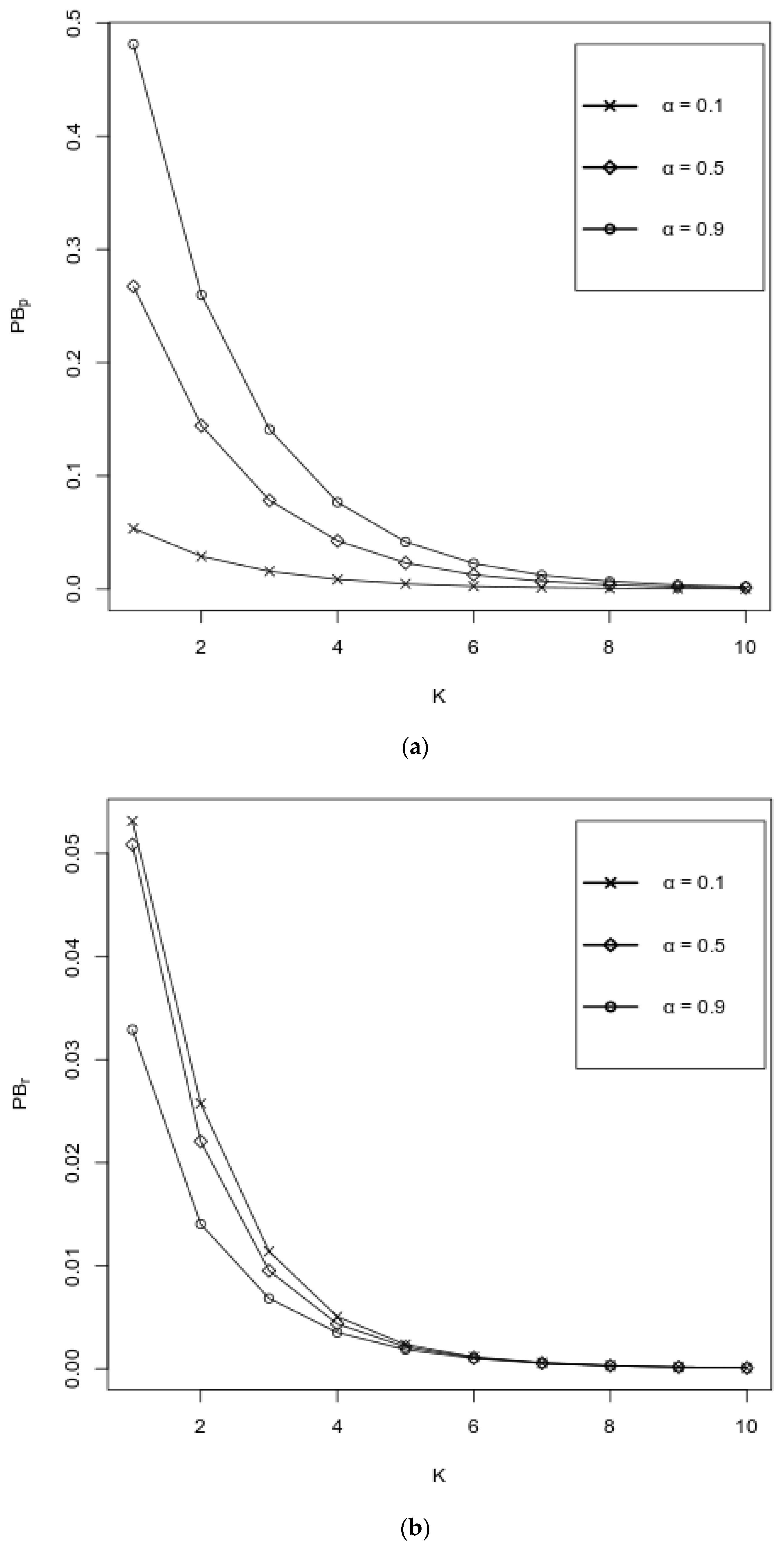
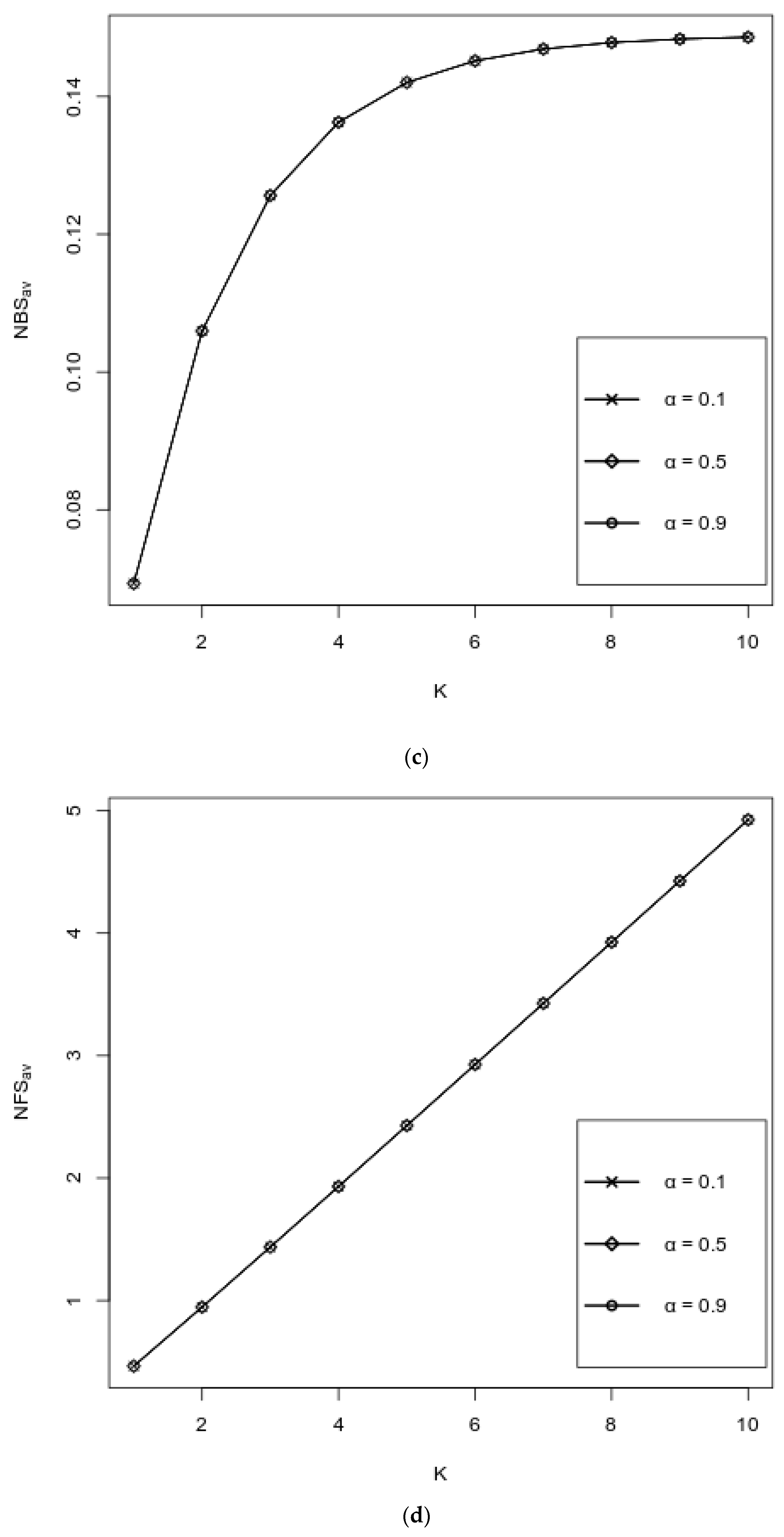
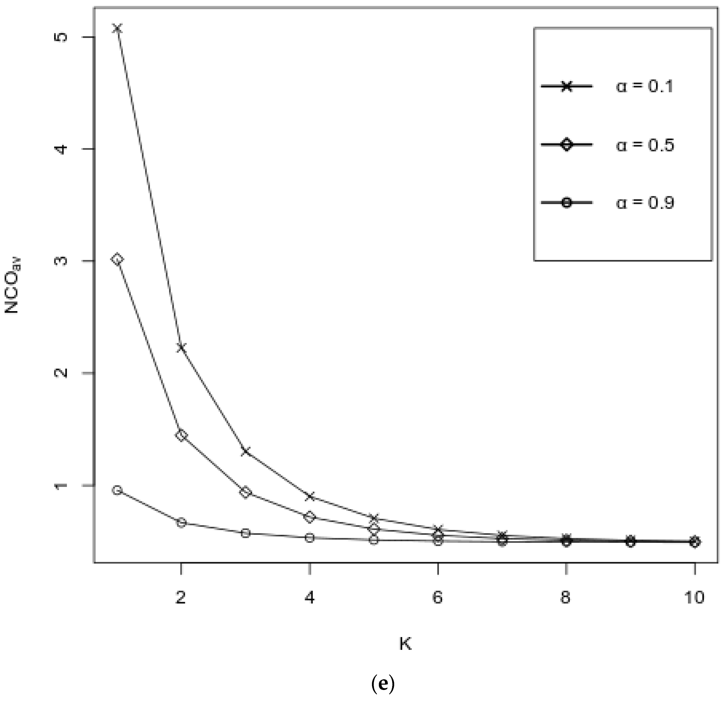
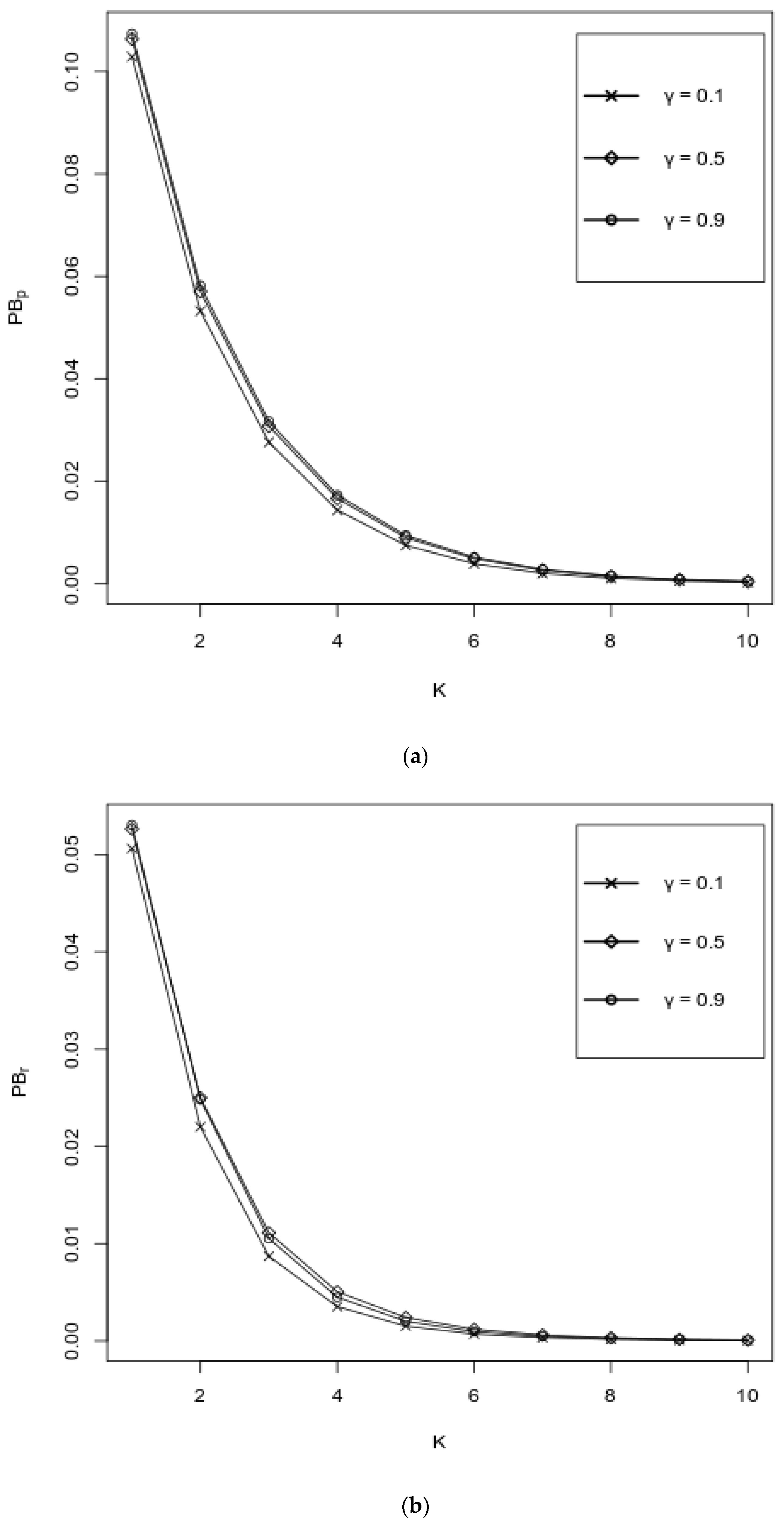
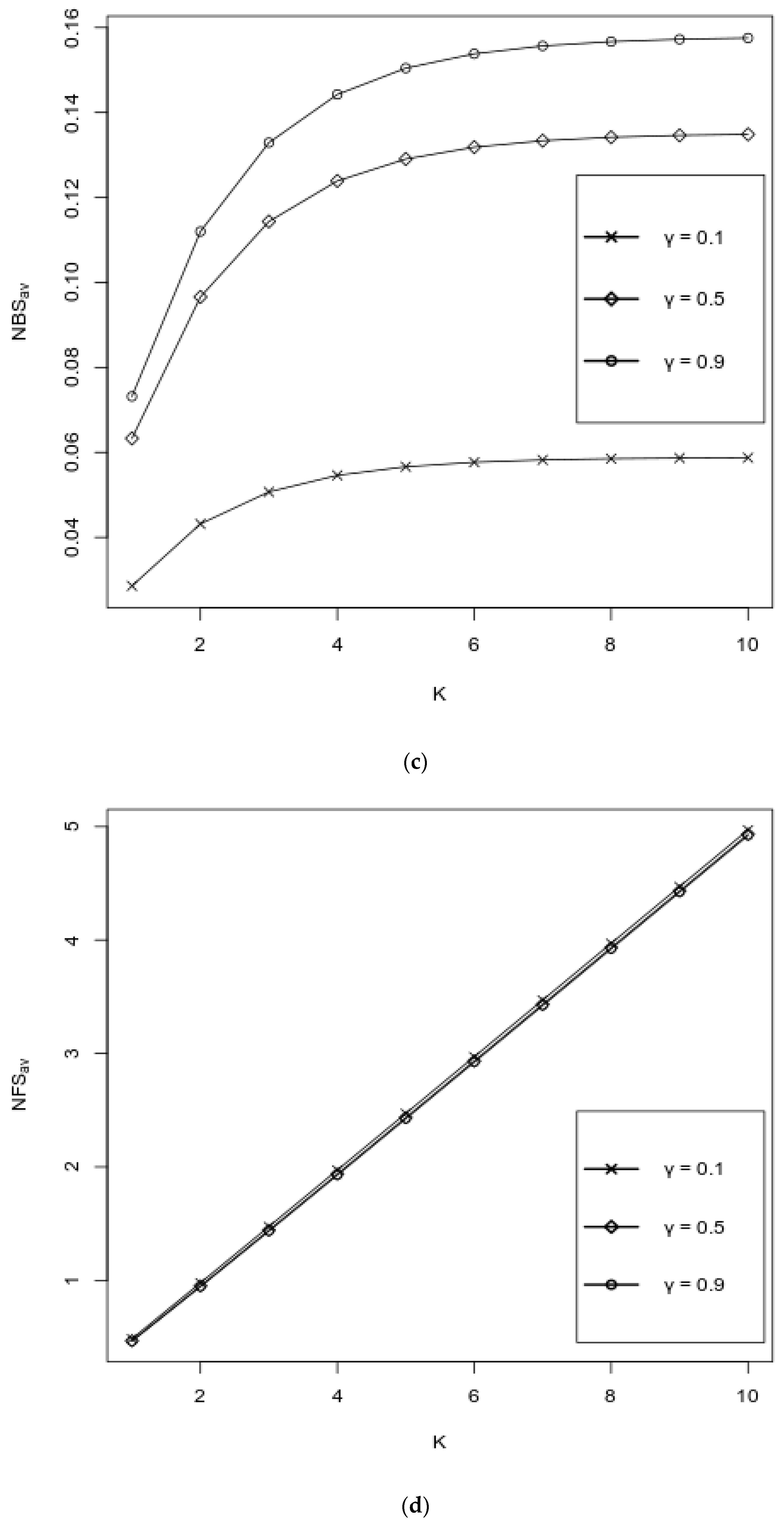
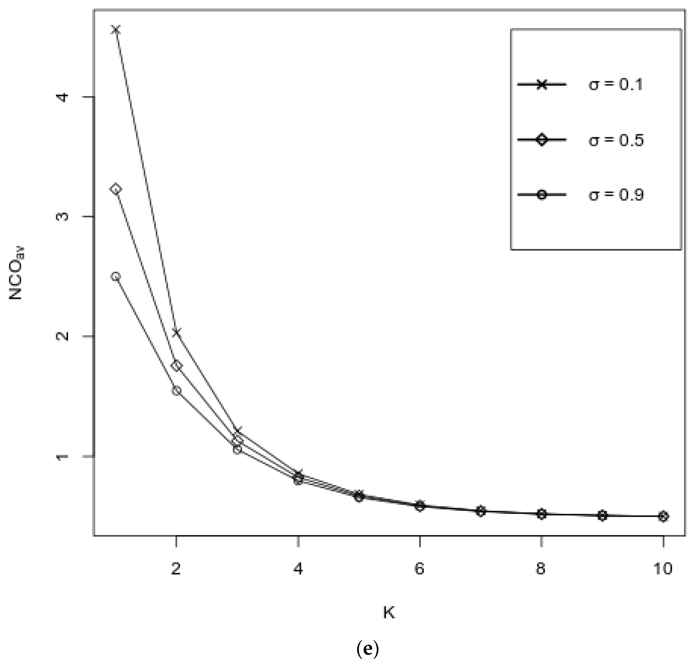
Figure 3a–e represent the behavior of performance measures as functions of K over various values of $\alpha$, where values of other probabilities are fixed as follows: $\beta =0.4,\gamma =0.7,\sigma =0.1$. It can be observed from Figure 3a,b that both $P{B}_p$ and $P{B}_r$ decrease with respect to K, where an increase of $\alpha$ is favorable for $P{B}_r$, whereas $P{B}_p$ increases with respect to $\alpha$; for large values of K, i.e., when K ≥ 7, the impact of the values of $\alpha$ is negligible. It is seen from Figure 3c,d that both the $NB{S}_{av}$ and the $NF{S}_{av}$ increase, and their values are almost independent of $\alpha$. Figure 3e exhibits the impact of K and $\alpha$ over the $NC{O}_{av}$. It is seen from the graph that the values of the decrease with respect to both K and $\alpha$. As in Figure 3a,b, here, when K ≥ 7, the impact of the values of $\alpha$ on the values of the $NC{O}_{av}$ is negligible.

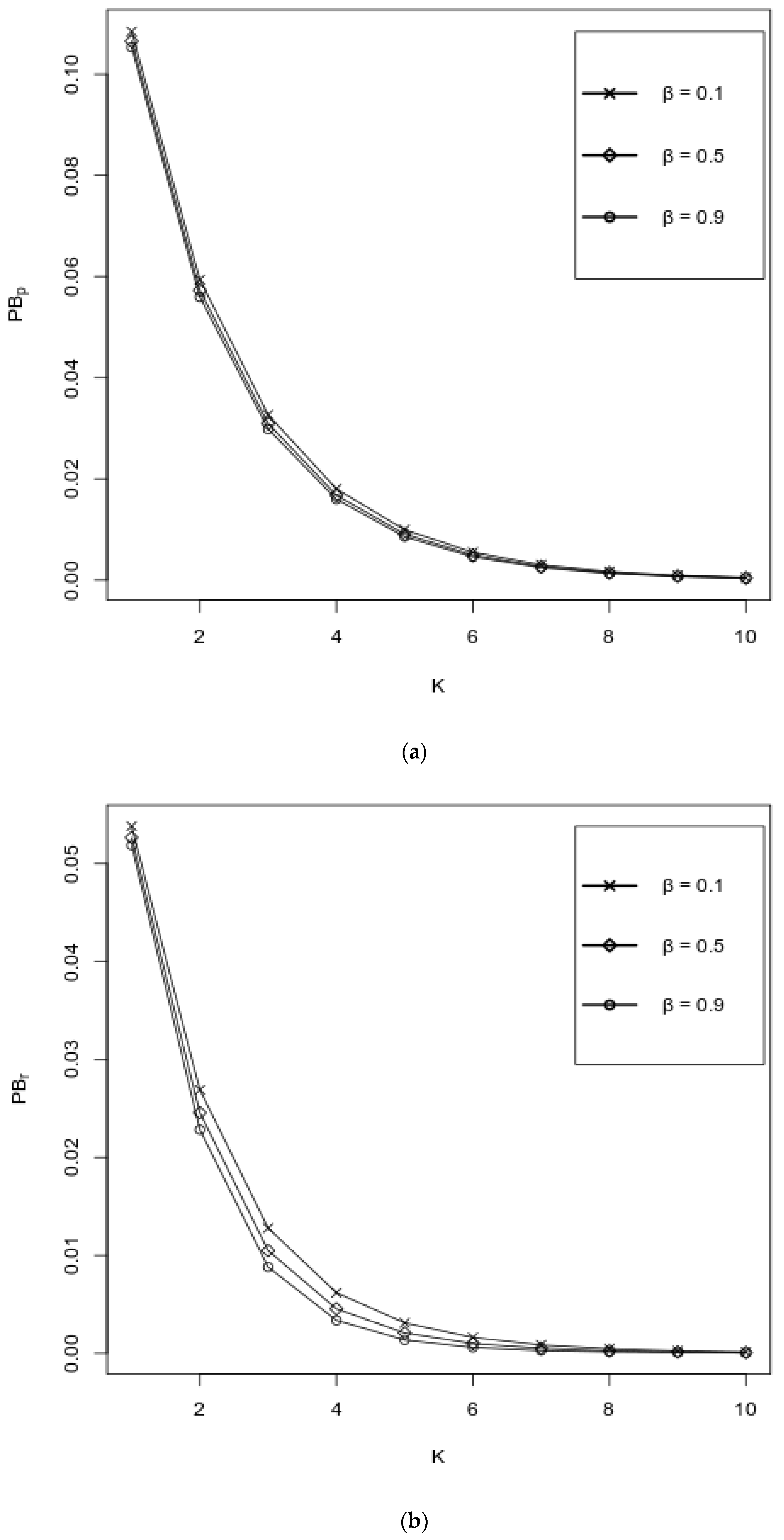
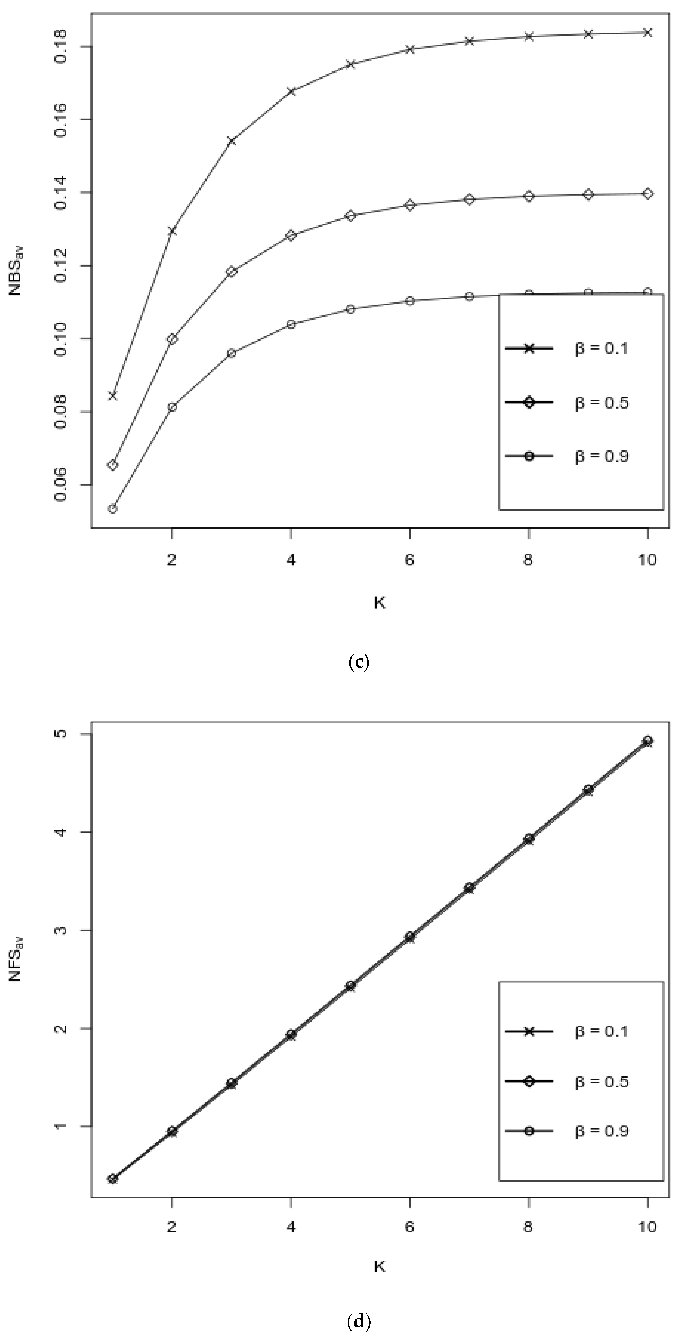
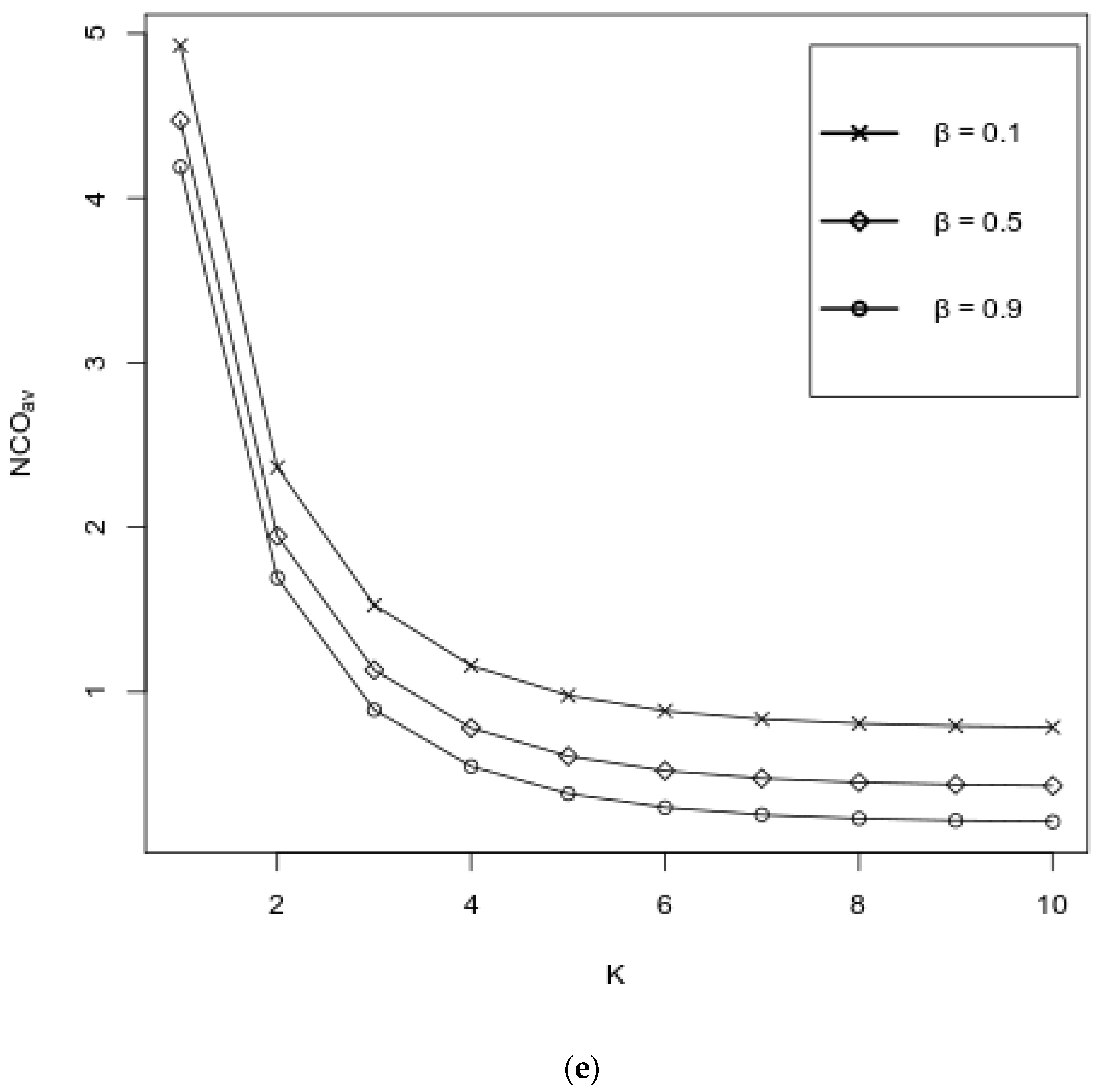
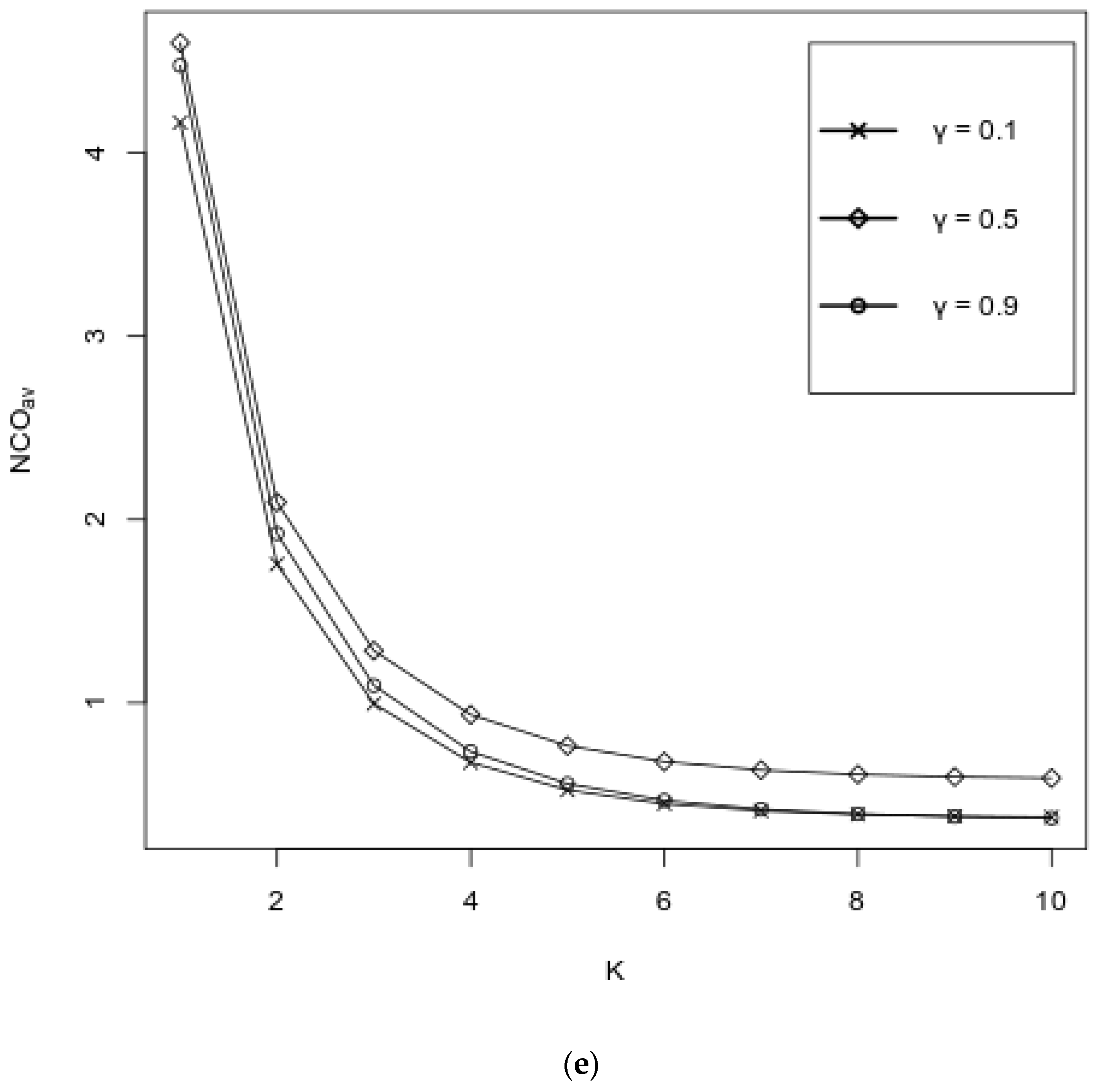
Figure 4a–e describe the behavior of performance measures as functions of K over various values of $\beta$, where values of other probabilities are fixed as follows: $\alpha =0.2,\gamma =0.7,\sigma =0.1$. It is seen from Figure 4a,b that both $P{B}_p$ and $P{B}_r$ decrease, and their values are almost independent on $\beta$; some dependence on $\beta$ is observed for $P{B}_r$ under small values of K, i.e., under small values of K, the performance measure $P{B}_r$ is decreasing by one with respect to $\beta$. As was expected, the $NB{S}_{av}$ increases with respect to K and decreases when $\beta$ increases (see Figure 4c). Figure 4d shows that the $NF{S}_{av}$ increases with respect to K, and its values are almost independent of $\beta$. However, it is seen from Figure 4e that the values of the $NC{O}_{av}$ increase with respect to K and decrease when $\beta$ increases, and that the impact of the values of $\beta$ on the values of the $NC{O}_{av}$ is essential for a large value of K.

Figure 5a–e show the behavior of performance measures as functions of K over various values of $\gamma$, where values of other probabilities are fixed as follows: $\alpha =0.2,\beta =0.4,\sigma =0.1$. From Figure 5a,b, we see that both $P{B}_p$ and $P{B}_r$ decrease with respect to K, and their values are almost independent on $\gamma$. Surprisingly, the $NB{S}_{av}$ increases when $\gamma$ increases (see Figure 5c). Such behavior of the $NB{S}_{av}$ can be explained as follows: for selected values of the load parameters of the system, an increase in the probability of a customer leaving the system from a broken server leads to an increase in the chance of p-customers being accepted, i.e., the average number of busy servers increases. Though, for other values of the load parameters, this performance measure might decrease when $\gamma$ increases. Figure 5d demonstrates that the $NF{S}_{av}$ increases with respect to K and its values are almost independent of $\gamma$. The impact of $\gamma$ on the values of the $NC{O}_{av}$ is negligible, and it decreases when K increases (see Figure 5e).

Figure 6a–e show the behavior of performance measures as functions of K over various values of $\sigma$, where the values of other probabilities are fixed as follows: $\alpha =0.2,\beta =0.4,\gamma =0.7$. Plot 6(a) exhibits that $P{B}_p$ is almost not affected by an increment in $\sigma$, and it decreases with the increasing number of servers. Conversely, plot 6(b) exhibits that, for a small value of K, $P{B}_r$ is affected by an increment in $\sigma$, but when K ≥ 7, the impact of the values of $\sigma$ is negligible and with increasing $\sigma$, $P{B}_r$ increases. Note that both the $NB{S}_{av}$ and the $NF{S}_{av}$ increase with respect to K, and the values are almost independent of $\sigma$ (see Figure 5c,d). It is seen from Figure 6e that for a small value of K, the $NC{O}_{av}$ is affected by an increment in $\sigma$, but when K ≥ 4, the impact of the values of $\sigma$ is negligible and with increasing $\sigma$, the $NC{O}_{av}$ decreases.

7. Conclusions

The present paper proposes mathematical models of unreliable multi-server RQwDFB. We studied both models with common finite and infinite orbit capacity for retrial and feedback customers. In a model with a finite orbit capacity, it is assumed that the probabilities of retrial, feedback, and balking from the orbit depend on the current number of customers in the orbit. For such a kind of model, we propose an exact method for calculating its steady-state probabilities as well as it performance measures. For a model with an infinite orbit size, an approximate space merging method is developed for calculating its steady-state probabilities as well as its performance measures.

As for directions for further research, it is proposed that models of RQwDFB with MAP flow and phase-type distributions of service time be studied. Practical interests are represented by the problems of optimizing RQwDFB regarding the selected criteria for the quality of their functioning. These problems are the subjects of future works.

References

- Phung-Duc, T. Retrial Queueing Models: A Survey on Theory and Applications. arXiv 2019, arXiv:1906.09560. [Google Scholar]
- Ayyappan, G.; Subramanian, A.M.G.; Sekar, G. M/M/1 retrial queuing system with loss and feedback under non-pre-emptive priority service by matrix-geometric method. Appl. Math. Sci. 2010, 4, 2379–2389. [Google Scholar]
- Ayyappan, G.; Subramanian, A.M.G.; Sekar, G. M/M/1 retrial queuing system with loss and feedback under pre-emptive priority service. Int. J. Comp. Appl. 2010, 2, 27–34. [Google Scholar] [CrossRef]
- Ayyappan, G.; Devipriya, G.; Subramanian, A.M.G. Analysis of single server queuing system with batch service under multiple vacations with loss and feedback. Math. Theory Model. 2014, 4, 79–90. [Google Scholar]
- Bouchentouf, A.A.; Belarbi, F. Performance evaluation of two Markovian retrial queuing model with balking and feedback. Acta Univ. Sapientiae Math. 2013, 5, 132–146. [Google Scholar]
- Choi, B.D.; Kim, Y.C.; Lee, Y.W. The M/M/c retrial queue with geometric loss and feedback. Comp. Math. Appl. 1998, 36, 41–52. [Google Scholar] [CrossRef] [Green Version]
- Korolyuk, V.S.; Melikov, A.Z.; Ponomarenko, L.A.; Rustamov, A.M. Methods for analysis of multi-channel queueing models with instantaneous and delayed feedbacks. Cybern. Syst. Anal. 2016, 52, 58–70. [Google Scholar] [CrossRef]
- Krishnamoorthy, A.; Manjunath, A.S. On Queues with Priority Determined by Feedback. Calcutta Stat. Assoc. Bull. 2018, 70, 33–56. [Google Scholar] [CrossRef]
- Melikov, A.Z.; Sztrik, J.; Aliyeva, S.H. Analysis of queuing system MMPP/M/K/K with delayed feedback. Mathematics 2019, 7, 1128. [Google Scholar] [CrossRef] [Green Version]
- Chang, C.J.; Ke, J.C.; Chang, F.M. Unreliable retrial queue with loss and feedback under threshold-based policy. Int. J. Ind. Syst. Eng. 2018, 30, 1–20. [Google Scholar] [CrossRef]
- Chang, F.M.; Liu, T.H.; Ke, J.C. On an unreliable-server retrial queue with customer feedback and impatience. Appl. Math. Model. 2018, 55, 171–182. [Google Scholar] [CrossRef]
- Jain, M.; Kaur, S. Bernoulli vacation model for M[X]/G/1 unreliable server retrial queue with Bernoulli feedback, balking and optional service. RAIRO-Oper. Res. 2020, 55, S2027–S2053. [Google Scholar] [CrossRef]
- Ke, J.C.; Liu, T.H.; Su, S.; Zhang, Z.G. On retrial queue with customer balking and feedback subject to server breakdowns. Commun. Stat. Theory Methods 2020, 1–17. [Google Scholar] [CrossRef]
- Mokaddis, G.S.; Metwally, S.A.; Zaki, B.M. A Feedback Retrial Queuing System with Starting Failures and Single Vacation. Tamkang J. Sci. Eng. 2007, 10, 183–192. [Google Scholar]
- Rajadurai, P.; Sundararaman, M.; Narasimhan, D. Performance analysis of an M/G/1 retrial G-queue with feedback under breakdown services. Songklanakarin J. Sci. Technol. 2020, 42, 236–247. [Google Scholar]
- Rajadurai, P.; Saravanarajan, M.C.; Chandrasekaran, V.M. A study on M/G/1 feedback retrial queue subject to server breakdown and repair under multiple working vacation policy. Alex. Eng. J. 2018, 57, 947–962. [Google Scholar] [CrossRef]
- Singh, C.J.; Kaur, S.; Jain, M. Waiting time of bulk arrival unreliable queue with balking and Bernoulli feedback using maximum entropy principle. J. Stat. Theory Pract. 2017, 11, 41–62. [Google Scholar] [CrossRef]
- Brian, P.C. Approximate Analysis of an Unreliable M/M/2 Retrial Queue. Master’s Thesis, Air Force Institute of Technology, Wright-Patterson Air Force Base, OH, USA, 2007; p. 84. [Google Scholar]
- Elhaddad, M.; Belarbi, F. Approximate analysis of an unreliable M/M/c retrial queue with phase merging algorithm. New Trends Math. Sci. 2016, 4, 9–21. [Google Scholar] [CrossRef]
- Raiah, L.; Oukid, N. An M/M/2 retrial queue with breakdowns and repairs. Rom. J. Math. Comp. Sci. 2017, 17, 11–20. [Google Scholar]
- Nazarov, A.A.; Sztrik, J.; Kvach, A.; Toth, A. Asymptotic sojourn time analysis of Markov finite-source M/M/1 retrial queueing system with collisions and server subject to breakdowns and repairs. Ann. Oper. Res. 2020, 288, 417–434. [Google Scholar] [CrossRef] [Green Version]
- Melikov, A.Z.; Fattakhova, M.I. Computational algorithms to optimization of buffer allocation strategies in a packet switching networks. Appl. Comp. Math. 2002, 1, 51–58. [Google Scholar]
- Liang, C.C.; Luh, H. Cost estimation queuing model for large-scale file delivery service. Int. J. Electr. Commer. Stud. 2011, 2, 19–34. [Google Scholar]
- Liang, C.C.; Luh, H. Optimal services for content delivery based on business priority. J. Chin. Inst. Eng. 2013, 36, 422–440. [Google Scholar] [CrossRef]
- Liang, C.C.; Luh, H. Solving two-dimensional Markov chain model for call center. Ind. Manag. Data Syst. 2015, 115, 901–922. [Google Scholar] [CrossRef] [Green Version]
- Neuts, M.F. Matrix-Geometric Solutions in Stochastic Models: An Algorithmic Approach; John Hopkins University Press: Baltimore, MD, USA, 1981; 332p. [Google Scholar]
- Korolyuk, V.S.; Korolyuk, V.V. Stochastic Models of Systems; Kluwer Academic Publishers: Boston, MA, USA, 1999; 185p. [Google Scholar]
Figure 1.
A graphical representation of the unreliable multi-server RQwDFB under investigation.
Figure 2.
State diagram for the split model with SS Er, K = 5.
Figure 3.
Loss probabilities of p-customers (a) and r-customers (b), the average number of busy (c) and failed servers (d) and the average number of r-customers in the orbit (e) versus the number of servers under various values of .
Figure 4.
Figure 5.
Figure 6.
Publisher’s Note: MDPI stays neutral with regard to jurisdictional claims in published maps and institutional affiliations. |
© 2021 by the authors. Licensee MDPI, Basel, Switzerland. This article is an open access article distributed under the terms and conditions of the Creative Commons Attribution (CC BY) license (https://creativecommons.org/licenses/by/4.0/).
Share and Cite
MDPI and ACS Style
Melikov, A.; Aliyeva, S.; Sztrik, J. Retrial Queues with Unreliable Servers and Delayed Feedback. Mathematics 2021, 9, 2415. https://0-doi-org.brum.beds.ac.uk/10.3390/math9192415
AMA Style
Melikov A, Aliyeva S, Sztrik J. Retrial Queues with Unreliable Servers and Delayed Feedback. Mathematics. 2021; 9(19):2415. https://0-doi-org.brum.beds.ac.uk/10.3390/math9192415
Chicago/Turabian StyleMelikov, Agassi, Sevinj Aliyeva, and Janos Sztrik. 2021. "Retrial Queues with Unreliable Servers and Delayed Feedback" Mathematics 9, no. 19: 2415. https://0-doi-org.brum.beds.ac.uk/10.3390/math9192415
Note that from the first issue of 2016, this journal uses article numbers instead of page numbers. See further details here.