
Periodic Solutions in Slowly Varying Discontinuous Differential Equations: The Generic Case


1
Department of Industrial Engineering and Mathematics, Marche Polytecnic University, 60121 Ancona, Italy
2
Department of Mathematical Analysis and Numerical Mathematics, Faculty of Mathematics, Physics and Informatics, Comenius University in Bratislava, Mlynská Dolina, 84248 Bratislava, Slovakia
3
Mathematical Institute, Slovak Academy of Sciences, Štefánikova 49, 81473 Bratislava, Slovakia
*
Author to whom correspondence should be addressed.
Mathematics 2021, 9(19), 2449; https://0-doi-org.brum.beds.ac.uk/10.3390/math9192449
Submission received: 8 September 2021
/
Revised: 23 September 2021
/
Accepted: 27 September 2021
/
Published: 2 October 2021
(This article belongs to the Special Issue Asymptotics for Differential Equations)
Abstract
:We study persistence of periodic solutions of perturbed slowly varying discontinuous differential equations assuming that the unperturbed (frozen) equation has a non singular periodic solution. The results of this paper are motivated by a result of Holmes and Wiggins where the authors considered a two dimensional Hamiltonian family of smooth systems depending on a scalar variable which is the solution of a singularly perturbed equation.
1. Introduction
In [1] a system like
has been considered, where , is Hamiltonian for any and has a one-parameter family of periodic solutions with period being in . As a matter of fact, in [1], is allowed to depend on and t being like and it is because of the t dependence of the perturbed equation that has been introduced. Indeed, introducing the variable mod T, the perturbed time dependent vector field is reduced to a time independent system on where is the unit circle. Then, they answered the following question: do any of these periodic solutions persist for ? They constructed a vector valued function that they called subharmonic Melnikov function which is a measure of the difference between the starting value and the value of the solution at the time in a direction transverse to the unperturbed vector field at the starting point. They proved that periodic solutions of the perturbed vector field arise near the simple zeros of .
Motivated by [1], in this paper we study Equation (1) in higher dimension and allowing to be more general than Hamiltonian and also discontinuous. As a matter of fact we assume that
where , , all functions here considered (i.e., , and ) are in their arguments, and is a small parameter. In this paper we study a non degenerate case where the unperturbed discontinuous system has a periodic solution for and certain non degenerateness conditions are satisfied. We construct a Jacobian matrix and show that, if it is invertible, the perturbed system has a unique periodic solution near the periodic solution of the unperturbed system. The Jacobian matrix being invertible does not allow the system to have a smooth family of periodic solution since in this case belongs to its kernel. We plan to consider this more degenerate case in a forthcoming paper.
We emphasize that the results of this paper easily extend to the case where is replaced by and , are smooth outside the singularity manifold . In this case in the unperturbed system
the term has to be replaced by . Finally, we observe that our results fit into a general theory of discontinuous differential equations presented in series of works [2,3,4,5,6,7,8,9].
2. Preliminary Results
We set
In the whole paper, given a vector v or a matrix A with , (resp. ) we denote the transpose of v (resp. A).
Let . We denote with the solution of (3) such that . We assume that exists such that the following conditions hold:
- there exists such that and for . Moreover,
- there exists such that for and . Moreover,
- )
- there exists such that for and .
Remark 1.(i) We may as well consider . As a matter of fact, changing with the roles of and are interchanged.
(ii) The first part of condition is equivalent to for and . Similarly, the first part of condition is equivalent to for and . Hence, being , in general we have
Similarly,
Hence (4) and (5) are stronger than the condition of existence of a continuous, piecewise , solution of the discontinuous equation such that for or , for and . Moreover, they are generic conditions having the important consequence that we do not need to define the vector field on the discontinuity manifold . Indeed, and imply transverse intersection of the solution with the discontinuity manifold . Heuristically, (4) implies that when a solution in , hits , it immediately leaves and enters . Similarly, condition (5) implies that when a solution in hits , it immediately leaves and enters . This case is referred to as thetransversecase. More generally, we have atopologically transversecase at , when
Of course there are other important cases arising in the applications. For example, it may happen that has a strong minimum at and
In this case the solution of the discontinuous systems is tangent to at and belongs to for . This case is referred to asgrazing. Another important case arising in the applications is theslidingcase. This happens when the inequalities
hold. These conditions force the solution to remain in the discontinuity manifold until one of the two conditions
or
arises first (it is assumed that these two conditions do not happen simultaneously). Here is the solution of a continuous differential equation on defined by means of the Filippov’s method [6] that takes into account the average of and at the points of . Then, if it is condition (8) that happens first, the solution re-enters into , while if it is (9) that happen first, the solution enter into .
In this paper we focus on the transverse case and , leaving the other cases to forthcoming papers. As we have already observed in the transverse case, there is no need to know the Filippov equation on .
For simplicity we set , , and
Then using it is easy to check that
Hence for , is a T-periodic solution of Equation (1) with , such that for all with and the following hold:
Now, let be an open ball of radius r centered at and L be a local hyperplane in passing through and transverse to . So
where . We have the following
Lemma 1.
Assume –. Then there exist open balls , such that for any there exist smooth functions , , and a continuous, piecewise function such that and the following hold:
- (i)
- as ;
- (ii)
- , for , and
- (iii)
- , for , and
- (iv)
- , for ,
- (v)
- for , , satisfies the differential equation , where the signs ± are taken accordingly to or .
Moreover, is a smooth map in the space of piecewise continuous functions and
as .
Proof.
Let and be two, sufficiently small, positive numbers such that . For we consider the equation
whose left-hand side vanish at , , . Moreover, the derivative with respect to t of the left hand side at , is
According to , possibly changing and , from the Implicit Function Theorem, it follows the existence of a smooth function such that
and
Next, since as it follows by continuity that
for some , uniformly with respect to . Hence (ii) holds with , for .
Then we see that exists such that, for , we have . Using the continuous dependence on the data we also see that
as and then
for . Hence (i) holds. Now, consider the solution of the equation
Note that, using the previous notation, we have
Note also that
for any .
It follows from the continuous dependence on the data that tends to , as together with its t-derivative, uniformly with respect to t in compact intervals such as , with sufficiently small. Next we consider the equation
in a neighborhood of . From (11)–(14) we get and
Then, the Implicit Function Theorem and an argument similar to the above imply that and a smooth function , with exist such that and (iii) holds with , . Moreover, by continuity,
Another argument of similar nature shows that iv) holds. Since all pieces of in the intervals , and consist of solutions of equation , it is easy to see that v) holds. The last conclusion follows from
as . □
Note that for it results if , if or and otherwise.
We set
Now, does this periodic, piecewise continuous solution persist when ? We have the following
Theorem 1.
Suppose – hold. Then there exist open balls , and such that for and there exist smooth functions , , and continuous, piecewise functions , such that , and the following hold:
- (i)
- as uniformly in ;
- (ii)
- , , for and
- (iii)
- , , for and
- (iv)
- , for and ;
- (v)
- for any ;
- (vi)
- for , , satisfies the differential Equation (1), where the signs ± are taken accordingly to or .
Moreover, is a smooth map in the space of piecewise continuous functions and
as , uniformly with respect to .
Proof.
Let be sufficiently small so that . For and , let be the solution of
From the continuous dependence of the data we see that
as . So, taking sufficiently small we get for . As a consequence there exists a unique such that
By the Implicit Function Theorem is a smooth function of . Moreover, from the last inequality in (18) we see that ii) holds and then intersects transversally at the point .
Repeating the above argument we see that, for , the equation
has a solution such that
from which we also get, using (17)
Moreover, by the Implicit function Theorem, there exists such that
and
Hence (iii) holds, i.e., at the point , points inward . Finally, by a similar argument we show that equation
has a solution such that
from which we also get, using (17)
Moreover, there exists such that
We set
and similarly
So, for any sufficiently small, say , we have . □
3. Periodic Solutions
In this section we prove a theorem concerning the existence of a periodic solution of system (1) such that
For let , , be the functions whose existence is stated in Theorem 1. We set
Note that the derivatives in the previous formulae are the derivatives of the restrictions of the various functions to . For example, denotes the derivative of and similarly for the other derivatives with respect to .
We prove the following
Theorem 2.
Suppose that – hold and that
Suppose, further, that the linear map :
has maximum rank (). Then there exists such that for system (1) has a unique periodic solution of period such that
and such that
Moreover, the map into the space of bounded functions is .
Remark 2.
(i) defines a matrix. However, it will be seen during the proof of Theorem 2 that
although this does not result immediately. This is why we made the assumption on the rank. By the way, because of (27) the assumption is equivalent to the fact that is an isomorphism. Note, also, that .
(ii) Condition (24) is a 0-average condition for at and implies that is a T-periodic solution of
Note that (24) corresponds to with in ([1], Theorem 3.1) where the authors search for subharmonic periodic solutions. Here, we do not have to take into account the extra parameter θ because of the autonomous character of Equation (1). Note, also, that, differentiating with respect to t, we get
and then
Proof.
Let , be as in Theorem 1. To obtain a periodic solution of Equation (1) we solve the system
for where is a small neighborhood of . When the second equation in (28) reads and is satisfied for any . So we replace (28) with
Since , the function
is in . Then, when (29) reads:
where and , because . From (10) it follows that equation has the solution . Next, since
we get
We now compute the Jacobian matrix of the left-hand side of Equation (30) at . We know that satisfies the integral equation
and that . More explicitly, taking into account the definition of :
Differentiating, we get
where
So, using , :
Similarly we have:
and hence
Since we see that
for any . Hence the assumption of the rank of is equivalent to the fact that is an isomorphism. From the Implicit Function Theorem it follows then the existence of such that for and , there exist , such that
Remark 3.(i) Note that, since , we have
Hence differentiating with respect to ξ and η:
and then
(ii) Suppose the following condition holds.
- (A)
- The linear maps and are both invertible.
For , , consider the function . From (10) we get ; moreover,
Hence there exists and a unique function such that and
For any the function is then a -periodic solution of the discontinuous equation . Next, suppose also that (24) holds, that is the equation
has the solution . We have
We prove that is invertible. Indeed, suppose that exists such that . Then
contradicting the fact that J is invertible. Note that, since , we get . So, if holds, besides –, we conclude that Equation (30) has the unique solution and the Jacobian matrix at this point is invertible. Thus the conclusion of Theorem 2 holds. In this case the invertibility of implies the existence of a family of periodic solution to the unperturbed equation ; however, the invertibility of J implies that only one of these solutions persists for the perturbed equation.
An Example
In this subsection we give an example of application of Theorem 2. The system we consider is
or, in matrix form:
where and
Note that
that is . Let . We prove the following result
Proposition 1.
For any , there exists a unique -periodic solution of
given by
where
Moreover, suppose that exists such that the function
has a simple zero at . Then there exists such that for there exist such that and Equation (38) has a unique, piecewise smooth, -periodic solution , intersecting transversally the discontinuity line and such that
Proof.
Note that the assumption on means that
and
For any , , we consider the point and set , where . Note that, for any , L is a transverse hyperplane in to
We prove that, for sufficiently small, assumptions – are satisfied at the point .
To this end we first describe the solutions of the unperturbed Equation (39) when , , , and such that is sufficiently small. We have
for all as long as , that is for all . As we get:
So
Being both conditions are satisfied if . Since we see that
Since , (44) is satisfied provided is sufficiently small. Indeed let . Then . So if . Note
for . Next, for , solves the equation:
until . Hence:
Note that and then, since , (45) holds for . Moreover,
Arguing as before, we see that holds if and only if and when , this last condition is equivalent to
i.e.,
It is easily seen that
Hence, if we get
for . Thus
provided is sufficiently small. Note that condition (46) implies and hence (ii) and (iii) of Lemma 1 hold. So for , and , (46) holds and then , , intersect transversally the negative axis at the point
Next, for , solves the equation:
for all such that . Hence
So:
for , since . Collecting all together, we see that, for and sufficiently small
Note that
hence for any with sufficiently small and . We obtain a -periodic solution of Equation (39) if and only if that is if and only if
and this holds if and only if or
Note that
and
Hence, for , Equation (38) has the unique (up to time translation) unstable -periodic solution:
For any , we have then a unique (unstable) -periodic solution of Equation (37), (or (38)) and we have seen that – are satisfied. Note that
hence
where , because of (41). Hence (24) in Theorem 2 is satisfied.
Next we compute the matrix . Recall that where . With reference to Lemma 1 we also have
so
and
Now differentiating (47) with respect to we get
Similarly:
So we get, after some algebra:
and similarly
Moreover, it is easy to check that
from which it easily follows that:
So
Note that, according to Remark 2, both and belong to . Next
As a concrete example we consider , where . We have
Now
and
Hence, when , the conclusion of Proposition 1 holds if the function has a simple zero at that is
4. Discussion
In this paper we study a persistence of periodic solutions of perturbed slowly varying discontinuous differential equations for a non degenerate case where the unperturbed discontinuous system (3) has a periodic solution for and certain non degenerateness conditions are satisfied. We construct a Jacobian matrix and show that, if it is invertible then the perturbed system has a unique periodic solution near the periodic solution of the unperturbed system. We plan to consider a more degenerate case in a forthcoming paper when (3) has a smooth family of periodic solutions.
Author Contributions
M.F. performed the investigation; F.B. designed the methodology. The contributions of all authors are equal. All authors have read and agreed to the published version of the manuscript.
Funding
This research was funded by the Slovak Research and Development Agency under the contract No. APVV-18-0308 and by the Slovak Grant Agency VEGA No. 1/0358/20 and No. 2/0127/20.
Institutional Review Board Statement
Not applicable.
Informed Consent Statement
Not applicable.
Conflicts of Interest
The authors declare no conflict of interest.
References
- Wiggins, S.; Holmes, P. Periodic orbits in slowly varying oscillators. SIAM J. Math. Anal. 1987, 18, 592–611. [Google Scholar] [CrossRef]
- Awrejcewicz, J.; Holicke, M.M. Smooth and Nonsmooth High Dimensional Chaos and the Melnikov-Type Methods; World Scientific Publishing Company: Singapore, 2007. [Google Scholar]
- Battelli, F.; Fečkan, M. On the Poincaré-Adronov-Melnikov method for the existence of grazing impact periodic solutions of differential equations. J. Diff. Equ. 2020, 268, 3725–3740. [Google Scholar] [CrossRef]
- di Bernardo, M.; Budd, C.J.; Champneys, R.A.; Kowalczyk, P. Piecewise-smooth Dynamical Systems: Theory and Applications. In Applied Mathematical Sciences; Springer: London, UK, 2008; Volume 163. [Google Scholar]
- Fečkan, M.; Pospíšil, M. Poincaré-Andronov-Melnikov Analysis for Non-Smooth Systems; Academic Press: Amsterdam, The Netherlands, 2016. [Google Scholar]
- Filippov, A.F. Differential Equations with Discontinuous Right-Hand Sides. In Mathematics and Its Applications; Kluwer Academic: Dordrecht, The Netherlands, 1988; Volume 18. [Google Scholar]
- Giannakopoulos, F.; Pliete, K. Planar systems of piecewise linear differential equations with a line of discontinuity. Nonlinearity 2001, 14, 1611–1632. [Google Scholar] [CrossRef]
- Kunze, M. Non-Smooth Dynamical Systems; Lecture Notes in Mathematics; Springer: Berlin, Germany; New York, NY, USA, 2000; Volume 1744. [Google Scholar]
- Leine, R.I.; Nijmeijer, H. Dynamics and Bifurcations of Non-Smooth Mechanical Systems; Lecture Notes in Applied and Computational Mechanics; Springer: Berlin, Germany, 2004; Volume 18. [Google Scholar]
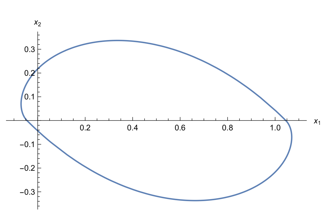
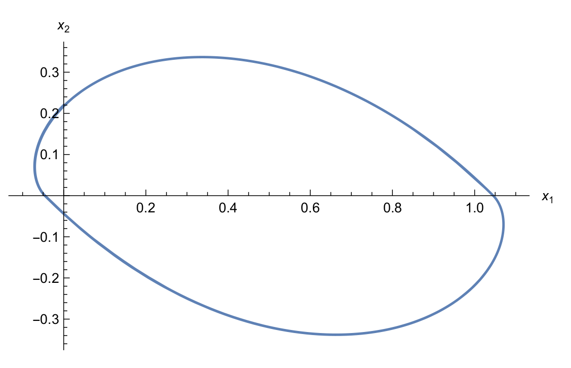
Figure 1.
Periodic solution of (56).
Figure 1.
Periodic solution of (56).

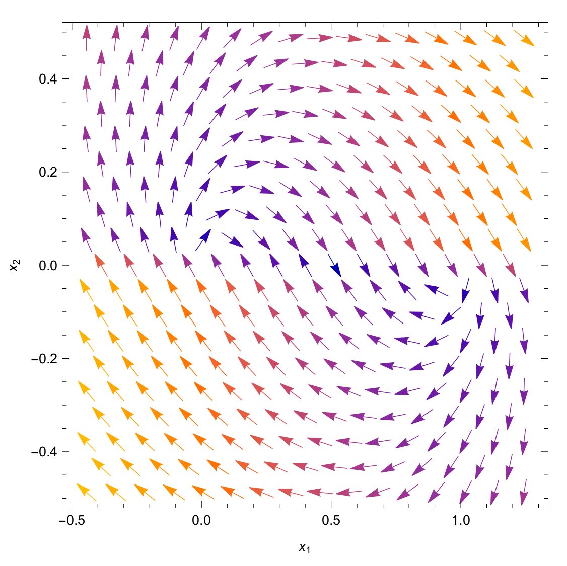
Figure 2.
Vector plot of (56).
Figure 2.
Vector plot of (56).

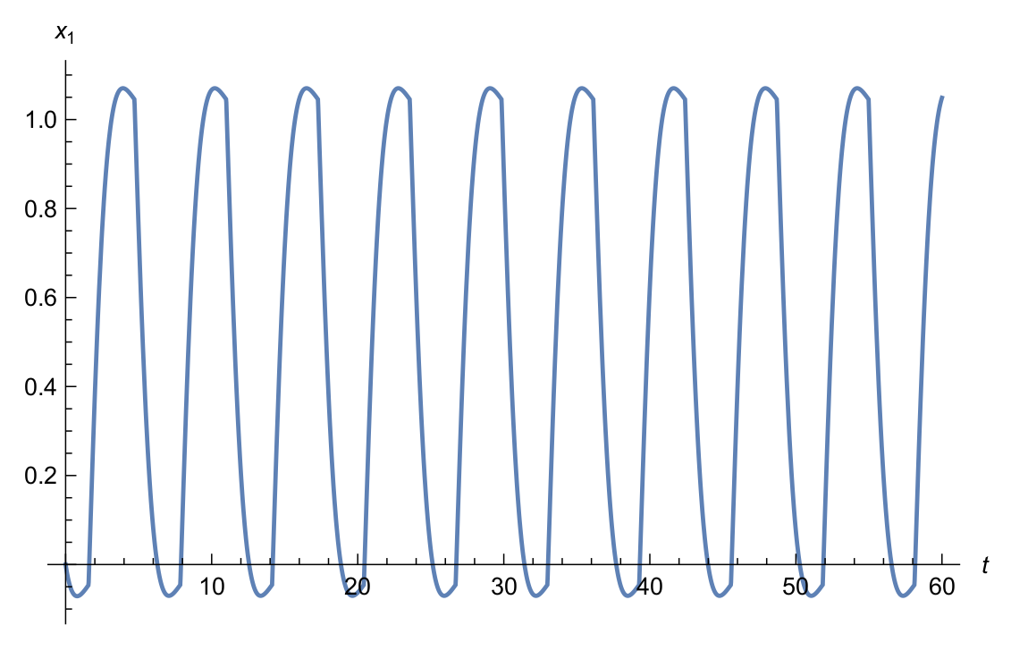
Figure 3.
component of periodic solution of (55) with .
Figure 3.
component of periodic solution of (55) with .

Figure 4.
component of periodic solution of (55) with .
Figure 4.
component of periodic solution of (55) with .

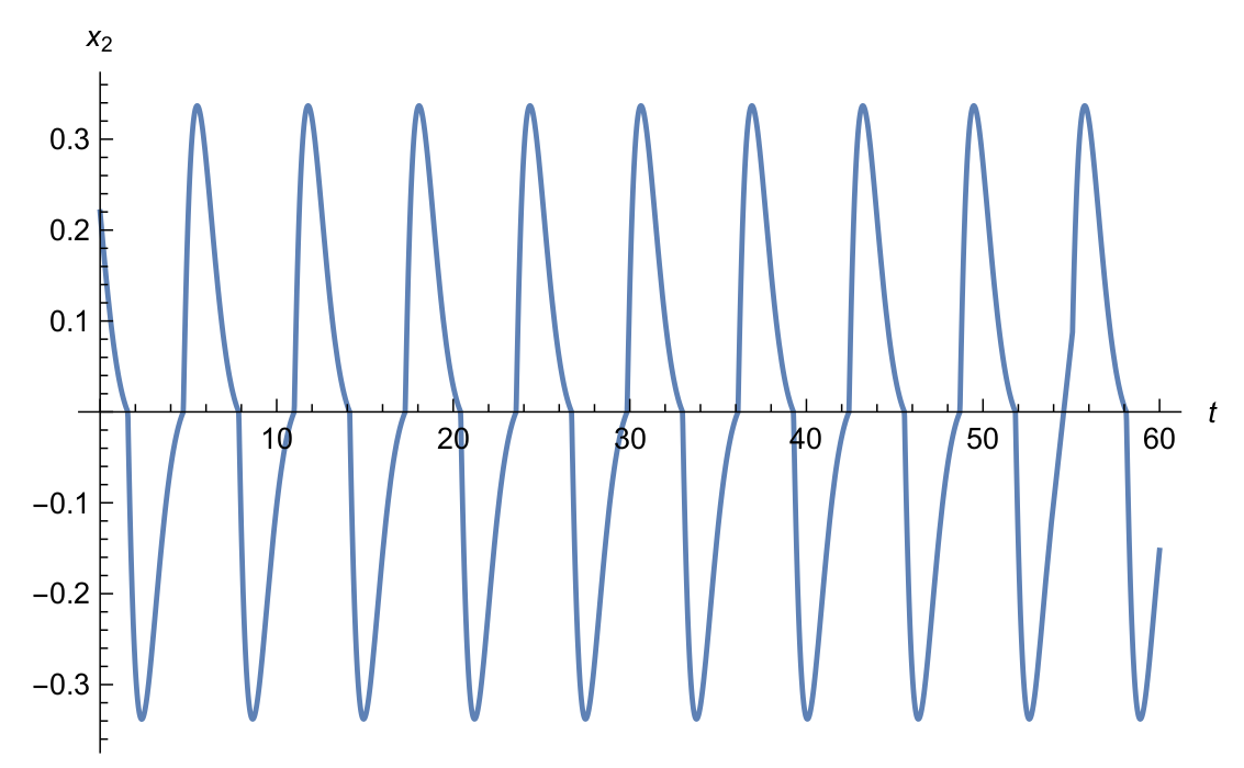
Figure 5.
component of periodic solution of (55) with .
Figure 5.
component of periodic solution of (55) with .

Figure 6.
component of periodic solution of (55) with .
Figure 6.
component of periodic solution of (55) with .

Publisher’s Note: MDPI stays neutral with regard to jurisdictional claims in published maps and institutional affiliations. |
© 2021 by the authors. Licensee MDPI, Basel, Switzerland. This article is an open access article distributed under the terms and conditions of the Creative Commons Attribution (CC BY) license (https://creativecommons.org/licenses/by/4.0/).
Share and Cite
MDPI and ACS Style
Battelli, F.; Fečkan, M. Periodic Solutions in Slowly Varying Discontinuous Differential Equations: The Generic Case. Mathematics 2021, 9, 2449. https://0-doi-org.brum.beds.ac.uk/10.3390/math9192449
AMA Style
Battelli F, Fečkan M. Periodic Solutions in Slowly Varying Discontinuous Differential Equations: The Generic Case. Mathematics. 2021; 9(19):2449. https://0-doi-org.brum.beds.ac.uk/10.3390/math9192449
Chicago/Turabian StyleBattelli, Flaviano, and Michal Fečkan. 2021. "Periodic Solutions in Slowly Varying Discontinuous Differential Equations: The Generic Case" Mathematics 9, no. 19: 2449. https://0-doi-org.brum.beds.ac.uk/10.3390/math9192449
Note that from the first issue of 2016, this journal uses article numbers instead of page numbers. See further details here.