
A Method to Automate the Prediction of Student Academic Performance from Early Stages of the Course


1
Department of Mathematics, Statistics and Computer Science, University of Cantabria, 39005 Santander, Spain
2
Department of Mathematics, University of Trento, 38122 Trento, Italy
*
Author to whom correspondence should be addressed.
Mathematics 2021, 9(21), 2677; https://0-doi-org.brum.beds.ac.uk/10.3390/math9212677
Submission received: 16 September 2021
/
Revised: 13 October 2021
/
Accepted: 15 October 2021
/
Published: 22 October 2021
(This article belongs to the Special Issue Advances in Artificial Intelligence and Statistical Techniques with Applications to Health and Education)
Abstract
:The objective of this work is to present a methodology that automates the prediction of students’ academic performance at the end of the course using data recorded in the first tasks of the academic year. Analyzing early student records is helpful in predicting their later results; which is useful, for instance, for an early intervention. With this aim, we propose a methodology based on the random Tukey depth and a non-parametric kernel. This methodology allows teachers and evaluators to define the variables that they consider most appropriate to measure those aspects related to the academic performance of students. The methodology is applied to a real case study obtaining a success rate in the predictions of over the 80%. The case study was carried out in the field of Human-computer Interaction.The results indicate that the methodology could be of special interest to develop software systems that process the data generated by computer-supported learning systems and to warn the teacher of the need to adopt intervention mechanisms when low academic performance is predicted.
1. Introduction
Recent technological innovations are currently reflected in the proliferation of groupware systems aimed at facilitating communication and coordination between users, as well as providing shared workspaces where users build artifacts that solve tasks. Collaboration supported by groupware is characterized by a large number of interactions that each user performs to cooperate with other members of a common group. An analysis of these interactions can be used to improve these collective processes. Duque et al. [1] propose a methodology for carrying out this analysis based on the following three phases:
- (i)
- to capture descriptive information of the interactions,
- (ii)
- to categorize and characterize the information collected and
- (iii)
- to intervene in the improvement of the collaborative activity.
Among these improvements, it is worth highlighting those that refer to providing better mechanisms to be aware of the interactions performed by other users [2], optimizing business processes to achieve strategic goals of organizations [3], and adapting academic processes supported by collaborative learning environments [4].
Computer-Supported Collaborative Learning (CSCL) is the research field that studies how groupware can be exploited in academic environments. Thus, groupware systems support processes that enable students to build new knowledge. These processes are usually oriented towards solving academic problems using social interaction with classmates. Students discuss and interchange ideas about solutions that solve a problem proposed by the teacher. Therefore, students acquire new knowledge due to the arguments and reasonings that arise in these discussions. One of the main research challenges in the CSCL field is building groupware that generate interventions in the collective process to optimize the student academic performance. Bravo et al. [5] define intervention mechanisms in CSCL systems with three components:
- (i)
- information to be processed by the students (analysis indicators to be displayed, advice to be shown, new exercise to be solved, etc.),
- (ii)
- a trigger moment or situation that puts the intervention in action,
- (iii)
- learners who receive each intervention.
1.1. Related Work
Intervention mechanisms have been deeply studied in the CSCL field to improve students learning. Thus, Anderson et al. [6] establish a set of theoretical principles to integrate software agents that simulate the role of a teacher who helps the student by issuing advice. Selker [7] follows this theoretical proposal with a generic architecture that allows modeling the behavior of the student and offering advice based on how users interact with the system. Meanwhile, Paolucci et al. [8] focus interventions in guiding students to solve academic problems. According to the criteria used by [9], it is possible to intervene in the work of students not only to optimize solutions but also to ensure optimal collaboration between classmates.
Some alternatives have already been explored to include artificial intelligence (in some of its variants) to the field of teaching, such as incorporating virtual assistants adapted to specific classes and different levels of students [10] or in online courses to mitigate the impact of the volume of students [11]. The aim of these intelligent systems is to provide continuous support to students, overcoming some of the disadvantages of online teaching, such as long response times by teachers or the correction of common errors. This support can be particularly interesting in courses based on significant problems in which the student learns by doing [12]. These methodologies can be applied in such a way that students are structured into groups that must carry out small tasks throughout the course. These tasks are related to each other in such a way that the solutions produced in one task are essential for the completion of the next tasks since they are taken as inputs [13]. Thus, students are increasingly producing larger solutions to more complex problems, generating at the end of the course a product close to the quality standards required in professional environments. Artificial Intelligence [14] can be used to analyze academic performance, being able to train different machine learning models [15,16] so that the different types of students are detected and classified. After extracting the characteristics of the students and classifying them, it can be given a series of warnings or personalized hints and feedback [17]. Therefore, Artificial Intelligence techniques are a useful tool to characterize learning activities and provide interventions. Intervention mechanisms have been generally focused on guiding specific activities. However, these research proposals do not provide information that enables teachers to guide a course or subject.
1.2. Our Research Contribution
This work is dedicated to propose a methodology that enables teachers to identify the factors with most impact in the academic performance of the students in a course, using an interaction and collaboration analysis of the earliest activities of the subject. The idea is to obtain a flexible methodology that can be adapted to any subject and software system that supports the learning process, individually or collaboratively. Thus, the intention is that the methodology does not adhere to predefined indicators or competencies, but rather that the teacher establishes, in a flexible manner, how to measure those aspects of the learning process that he/she considers of interest. Additionally, the methodology is based on a statistical technique that can be carried out in an automated manner by software tools. Therefore, the amount of information generated by CSCL systems is not an obstacle for the execution of the prediction process, as is automated by software support. Thus, a generic and flexible solution is obtained, providing a state of the art proposal that automates the process of predicting academic performance while providing the teacher with the freedom of configuration, not sticking to specific competencies or indicators. This methodology is useful to intervene, not only in specific problem-solving activities but also in adapting the course development to the students. It is based on statistical data depth [18] and non-parametric kernel classification [19] and is here applied to the Human-computer Interaction subject of the Computer Science degree at the University of Cantabria.
This paper has four additional sections. Section 2 describes the methodology for predicting the academic performance of the students from the interactions collected in early stages. Section 3 shows the results of a case study in which the methodology is applied to predict academic performance in a university course. Section 4 discusses the results of this work. The computations have been carried out using the R software.
2. Materials and Methods
Our main research problem is about knowing whether it is possible to predict successfully the performance of students in an academic course from the earliest activities supported by groupware, by making use of the performance of the students who took the course in previous years. Denoting by the amount of tasks performed by the students, the research problem is divided into the following research subproblems:
- 1.
- Is it possible to predict successfully the average grade over the N tasks based on the two first tasks performed by the students?
- 2.
- Is it possible to predict successfully the average grade over the N tasks based on the three first tasks performed by the students?
- 3.
- Is it possible to predict successfully the average grade over the N tasks based on the four first tasks performed by the students?
- 4.
- Is it possible to predict successfully the average grade over the N tasks based on the five first tasks performed by the students?
To design a methodology that allows for this, the following three types of data, commonly used to characterize groupware [20], are taken as input:
- Communication between classmates: These data measure the fluency in exchanging ideas on how to solve the activities (e.g.: contributions from each student, perception of the quality of the proposals of others, etc.).
- Coordination to distribute tasks: These data allow us to quantify how the efforts are distributed between the members of the group (e.g.: hours of work of each member of the group, perception of the effort of the classmates, etc.).
- Collaboration for building quality solutions: These data quantify whether the collective process allowed the student to improve solutions (e.g.: grades in collaborative activities, perception of how solutions are improved by the classmates, etc.).
The measurement of the students’ academic performance was carried out through the analysis indicators proposed by [5]. This proposal includes a set of indicators that measure three dimensions of the students’ academic work:
- 1.
- The individual work of the students. Examples of these indicators are the number of proposal of each learner and the amount of individual interaction with the solution.
- 2.
- The degree of collaboration. Examples of these indicators are the number of proposals commented by other learners and the degree in which the task distribution was equitable.
- 3.
- The solutions generated. Examples are the degree to which the solution is well-formed according to the syntax rules of the programming language and the assessment of whether the solution solves the task goals.
Finally, the technological framework proposed by [21] was used to automate the calculation of a single variable that measures student performance as an average of the value of these indicators. Each indicator has the same weight in the calculation of the final variable. These data are multivariate and are processed by means of data depth to reduce their dimensionality, resulting in univariate data, which allows to easily predict the students performance. This prediction is done in terms of non-parametric supervised classification. We employ the random Tukey depth [22] as statistical data depth. As this is a more novel technique, we explore it in what follows. After that, we propose the methodology employed in practice and introduce the studied dataset.
2.1. Statistical Data Depth
According to the recent paper [23], statistical depth is a current hot research topic in statistical analysis [24,25,26,27,28] in some papers on the topic. Given a probability distribution P on a statistical depth function orders the points in from the “center of P” to the “outer of P”. Obviously, this problem includes data sets if we take P to be the empirical distribution associated to the dataset at hand. Note that in the one-dimensional case this order is trivial; being reasonable to order the points using the order induced by the function
This implies that the data is ordered using the decreasing order of the difference between 50 and their percentiles, in absolute values, and the deepest points are the medians of P. Ordering multivariate data is, however, neither trivial nor pursued in a unique manner. Therefore, several multidimensional depths have been proposed [29,30,31,32]. Here we are mainly interested in the random Tukey depth function, which is a random approximation of the Tukey (or halfspace) depth [33]. The problematic of the Tukey depth is the required high computational time [34]. This issue is addressed by its random approximation. According to Zuo and Serfling [18], the Tukey depth behaves very well in comparison with the existing competitors. The random Tukey depth inherits the good theoretical properties of the Tukey depth and, in particular, that it characterizes discrete distributions [35], which comes in handy. for the study performed in this paper.
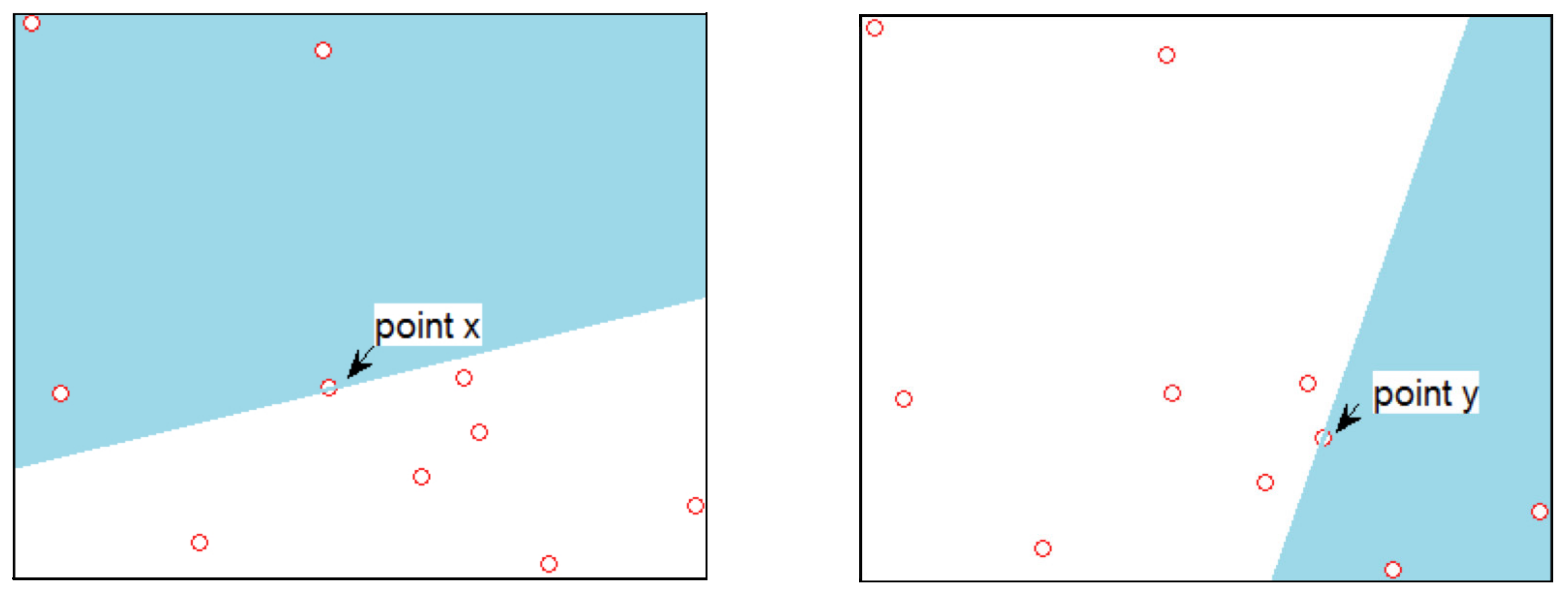
For , the random Tukey depth of x with respect to , is the minimal probability which can be attained over a set of randomly closed halfspaces containing i.e., is the minimum of the one-dimensional depths (see (1)) of a finite number of randomly chosen one-dimensional projections of x, where those depths are calculated with respect to the corresponding marginal of P. In this paper we make use of 50 random projections. Let us, then, concentrate further on explaining what the idea of deepness inside the definition of random Tukey depth is. Given n points, let us denote one of them by Then, we want to compute the random Tukey depth of x with respect to the set of n points. For that, we compute the number of points in the set that are contained in each of the randomly chosen closed halfspaces that has x in its border. Then, we record any of those halfspaces that contain the fewest points from the set and the depth of x is this number of points divided by In the left-hand side plot of Figure 1, in n is equal to ten and the random Tukey depth of x is given, among others, by the randomly obtained closed halfspace painted in pastel blue. As there are four points inside this halfspace, the random Tukey depth of x is Note that x is the deepest point in the set. From the right-hand side plot of Figure 1 we can observe that, taking sufficient randomly chosen halfspaces, the random Tukey depth of point y is because among all the closed halfspaces that have y on their border, the ones that contain fewer points from the set do contain three points. Alternatively, taking into account that (1) coincides with the definition of random Tukey depth in to compute the random Tukey depth of a point with respect to a set of size n we can do the following. For each randomly selected vector v in the unit sphere of we compute the one-dimensional depth, (1), of the projection of x on v with respect to the projection of A on Then, the minimum of the one-dimensional depths over the drawn is the random Tukey depth of Note that when A is finite it suffices to take an amount of vectors, equal to the number of combinations of elements taking at a time without repetition.
2.2. Methodology in Practice
To evaluate the performance of the students, we make use of their grades. There are a variety of grade systems. For instance:
- A letter in the set with the highest possible grade and U the lowest. This is a common grading system in the United Kingdom.
- A number in the set with 1 the highest possible grade and 5 the lowest. This is the system used in Germany.
- A number in the interval [0, 10] with 0 the lowest possible grade and 10 the highest. This system is the one established in Spain.
The methodology we present here is valid for any grading system. The reason is that any system can be translated into a success percentage. That is, any grade can be transformed into a number with the percentage of right answers, for instance. Thus, to particularize it, we focus on the Spanish grading system.
Let be the dataset under study where for any with both larger than two. represents the grades of student Thus, if we have theoretically recorded 6 grades for each student. Missing grades will be assigned the lowest possible grade. The dataset is split into training sample, and test sample Thus, and for any and Then, each and, analogously, each Let The objective in this manuscript is to predict the average grade for each making use of:
As a large range of grades are possible in the Spanish system, we summarize it by substituting by that provides the membership of to one of the intervals in the following set:
These intervals have been set by taking into account that a student passes with a grade larger or equal than 5. Thus, we use the interval [0,4) for those grades where the student clearly fails. The largest possible grade posses also an interval, {10}, since it is a distinction.
Then, noting that G in (5) denotes the set of all labels, it is easy to see that we are given a series of data with label:
- the training sample consists of the pairs for ,
- the test sample is given by the pairs forwhere, for each , provides the membership to the intervals inof Note that these intervals are of larger length, to emulate confidence bands.
The idea is to first construct a model making use of the training sample. To construct it, we simply employ a supervised classification procedure where first the random Tukey depth is used to reduce the dimensionality, and then a normal kernel classifier is applied to perform the classification. In what follows we explain in what consists this classifier; for which we refer to Ferraty and Vieu [36] and Ferraty and Vieu [37], Chapter 8 for more technical details, consistency, and rate of convergence of posterior probabilities. For that, we suppose that and and , are independent and identically distributed (i.i.d.) as where X takes values in and Y takes values in G. The classifier is based on a general Bayes classification rule. For a general pair , where and , it is defined the posterior probability
Note that P denotes the underlying probability. Then, is classified to the class yielding maximum posterior probability. In particular, for classifying points in the training sample we take for some , while for classifying points in the test sample for some For this purpose, we need to estimate . As the training sample , consists of i.i.d. copies of , we use it to estimate the underlying probability distribution. Specifically, we replace by its Nadaraya–Watson estimator [38,39], which is given by
where , is the Euclidean norm on , and K is a probability kernel satisfying , for , and it is non-increasing in for u is positive. Notice that the sum at the numerator is only over those i such that yielding
Additionally, the closer the point x is to , the closer the quantity is to 0, the maximal point of the kernel thus, yielding a higher probability. Specifically, we choose K to be 2 times the standard normal density if u is non-negative and 0 otherwise. The parameter h is chosen so that the classification error in the training sample is minimized. Then, we introduce into the model the for and obtain the predictions of the
2.3. The Dataset
The proposed method was applied in the Human-computer Interaction (HCI) subject taken by students in the third year of the Computer Science degree at the University of Cantabria, in Spain. The HCI discipline deals with studying how people interact with computers. Some of the main objectives pursued by this discipline are the definitions of methodologies to develop more efficient and intuitive user interfaces, the creation of methods that allow evaluating and comparing the characteristics of user interfaces and the design of models that allow the interaction between people and computers to be represented. HCI studies the relationship of people with computers and this makes it necessary to apply knowledge from fields as varied as Psychology, Computer Science, Telecommunications and Sociology. Therefore, HCI has a multidisciplinary nature that bases it on many classical fields of knowledge.
This subject follows a Project-Based Learning (PBL) approach through tasks in which students work collaboratively to design and build different types of user interfaces (for mobile phones, web applications, or desktop tools). The methodology is applied to predict academic performance using data from a few early activities. The main goal of this experimentation is to identify elements of the learning process (tasks, group composition, etc.) that should be intervened to have a real impact in the academic performance of the students in a course.
Data collected quantify the activity of 205 students:
- 43 of them took the subject during the academic period 2017/18,
- 41 during 2018/19,
- 63 during 2019/20 and
- 61 during 2020/21.
As part of their academic course, these students performed 6 tasks that required designing user interfaces. These tasks are the following:
- 1.
- Prototype a mockup of a user interface for smartphones.
- 2.
- Build user interfaces using the Android platform.
- 3.
- Design and build user interfaces for desktop computers using a WIMP (windows icons menus and pointers) style.
- 4.
- Design and build user interfaces for desktop computers using a WYSIWYG (What You See Is What You Get) style.
- 5.
- Design and build the user interfaces of a website.
- 6.
- Perform a usability test process.
Software support used by the students was a videoconferencing tool with a shared whiteboard and chat, a shared folder and Axure, a UX tool to prototype interfaces. These user interfaces were later built using Android technologies and Java and HTML languages. Students collaborated in groups, resulting in a total of 79 groups:
- 14 of them for the academic period 2017/18,
- 15 for 2018/19,
- 21 for 2019/20 and
- 29 for 2020/21.
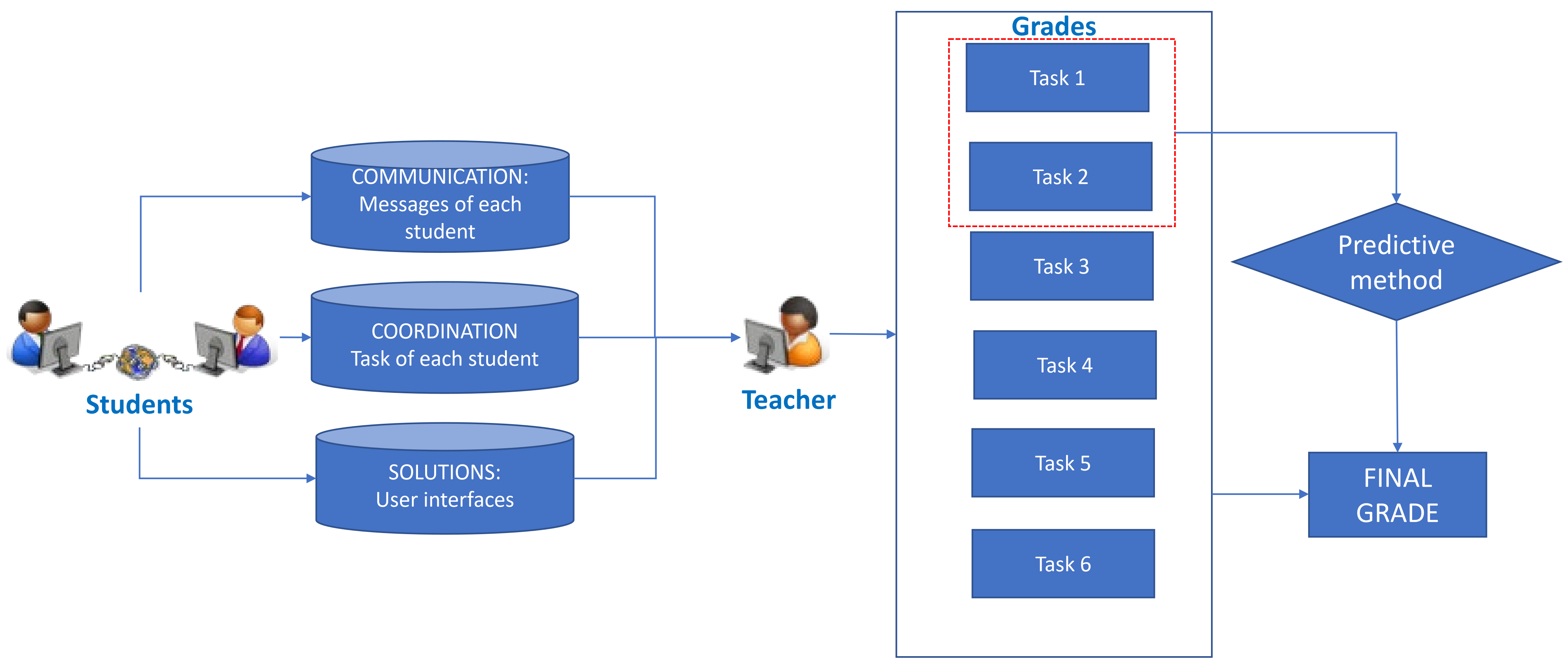
The dataset was used to experiment with the proposed methodology as shown in Figure 2. The students collaborated in groups to solve the proposed tasks. This collaboration was made with the support of software tools that recorded their communications, how the workload was distributed, and the solutions to the tasks. The teacher used all this information to grade each assignment. Finally, the methodology was applied to verify if a small number of tasks allowed to predict the final grade of the student.
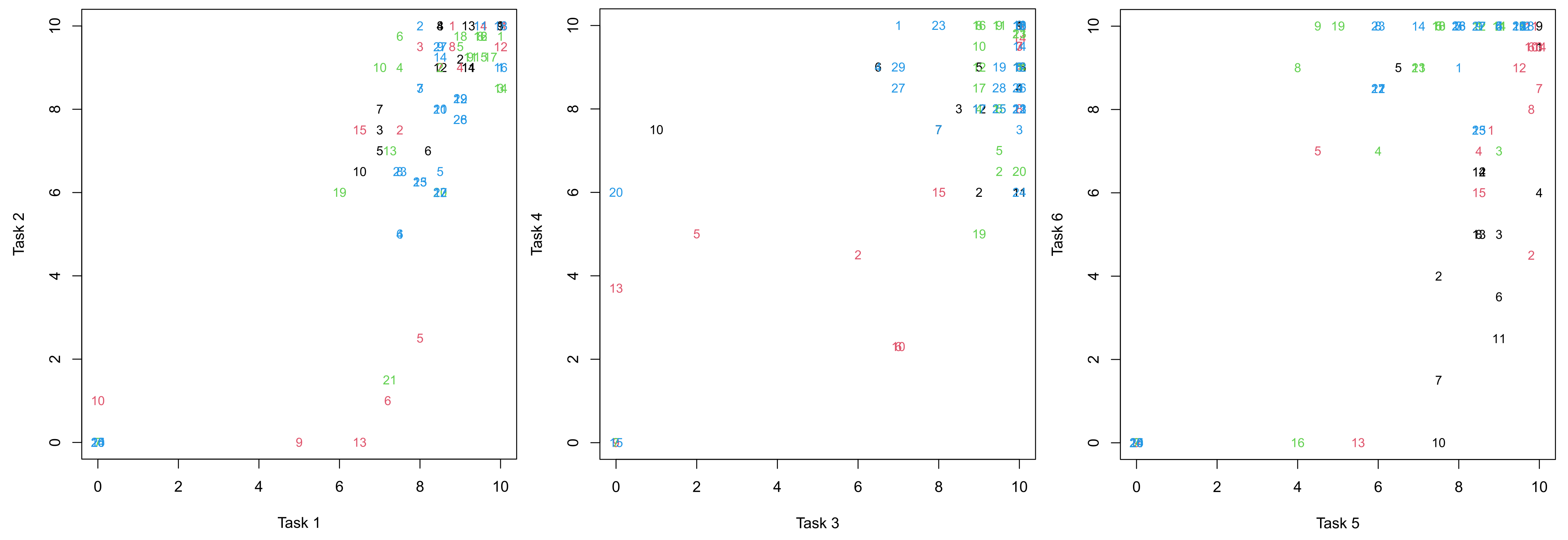
To illustrate the dataset, we have plotted in Figure 3 the grades of the groups over the six tasks of the different academic periods. These grades are in the range 0–10, 0 being the lower possible grade and 10 the highest one. These grades are the result of quantifying the following three aspects:
- (i)
- the quality of the user interfaces,
- (ii)
- the extent to which group members distribute the workload equitably, and
- (iii)
- the contributions and proposals that arise to establish a real collaboration.
The left plot corresponds to the grades in Task 1 against those in Task 2, the central plot to those in Task 3 against those in Task 4 and the right plot to those in Task 5 against those in Task 6. The grades of the academic period 2017/18 are represented in black, those of 2018/19 in red, those of 2019/20 in green, and those of 2020/21 in blue. In each of these academic periods we have labeled each group by a number. Thus, we can observe, for instance, that:
- Group 3 of the academic period 2017/18 had grades in the interval [6,8) in Tasks 1 and 2 that improved to the range [8,10) for Tasks 3, 4 and 5 and decreased to the range [4,6) for Task 6.
- Group 5 of the academic period 2018/19 had grades in the range [8,10) in Task 1 that worsened to the range [2,4) for Tasks 2 and 3 and slighted improved to the interval [4,6) for Tasks 4 an 5 and again improved to the interval [6,8) for Task 6.
- Group 19 of the academic period 2019/20 had grades in the range [6,8) in Tasks 1 and 2 that improved to the range [8,10) for Tasks 3, decreased to the range [4,6) for Tasks 4 and 5 and then highly increased to a 10 for Task 6.
This leads us to realize that the patterns among the different groups is different, which makes the analysis more difficult.
3. Results
The objective of this section is to provide the results for the research problem proposed in Section 2, which consist in predicting the average grade of the students taking an academic course based on their early performance in the course and the performance of the students who took the course in previous academic years. In particular, we use the grades of the courses 2017/18, 2018/19, 2019/20 as training sample; obtaining a training sample of size We use as test sample the early grades recorded during the course 2020/21 to predict the average grade over the six tasks (in groups); having a test sample of size The research problem has four subproblems where the first one regards as early grades the first two, the second research problem the first three grades, the third the first four grades, and the fourth problem the first five grades. Making use of the methodology expressed in Section 2, we perform here a supervised classification to predict the average grade over the six tasks of the groups in the test sample. To do this, we take the amount of tasks done by the student, in the range from 2 to 5.
At the top of Table 1 we observe the results of applying the model to the test data with (research problem 1). That is, we have constructed the model making use of the training data which are the grades for the first two Tasks, and the label which is the average grade of the six Tasks, for Then, we have reported in the top panel of Table 1 the summary of the range values that is, the estimated values of We report the values by providing a wider ranger, of a ± grade, than the one used to summarize the given values. Thus, we obtain that the three test groups of students whose average grade is in the interval [0,4) are correctly classified in the interval [0,4]. Analogously, the four groups of students with average grade in the interval [7,8) are appropriately classified in the interval [6,8].
There are 13 groups of students in the average grade range [8,9), 3 of them are classified in the [6,8] interval and the other 10 in the [7,9]. Although both classifications should be considered correct, to be on the safe side, we have only considered successful for a later analysis (Figure 4) those classified in [7,9]. Similarly, there are seven groups of students with average grade in [9,10) which are correctly classified in [8,10] and another one which is not so clear as it is classified in [7,9]. Thus, for the later analysis we only consider as correct the seven classified in [8,10]. Furthermore, there is one case in the analysis that is clearly wrongly classified. That is the one of the group of students with average grade in [9,10) whose estimation is in [6,8].
When making use of the grades of Tasks 1, 2, and 3 (research problem 2) to predict the average grade over the six tasks, the obtained results when classifying test sample are, as expected, slightly better than those obtained by just using Tasks 1 and 2 (research problem 1) and worse than when also using Task 4 (research problem 3). They are reported in the second block of Table 1. In particular, we can observe only one clear misclassification, which is that of a group with an average grade in the interval [0,4) whose estimated average grade belongs to the interval [6,8]. The results obtained when making use of just Tasks 1, 2, 3, and 4 (research problem 3) are the same than those obtained when also adding Task 5 (research problem 4). In particular, the absolute number of misclassifications increases to two in both cases. As reported in Table 1, they correspond to groups with average grade in the interval [0,4) that is estimated as in the interval [6,8].
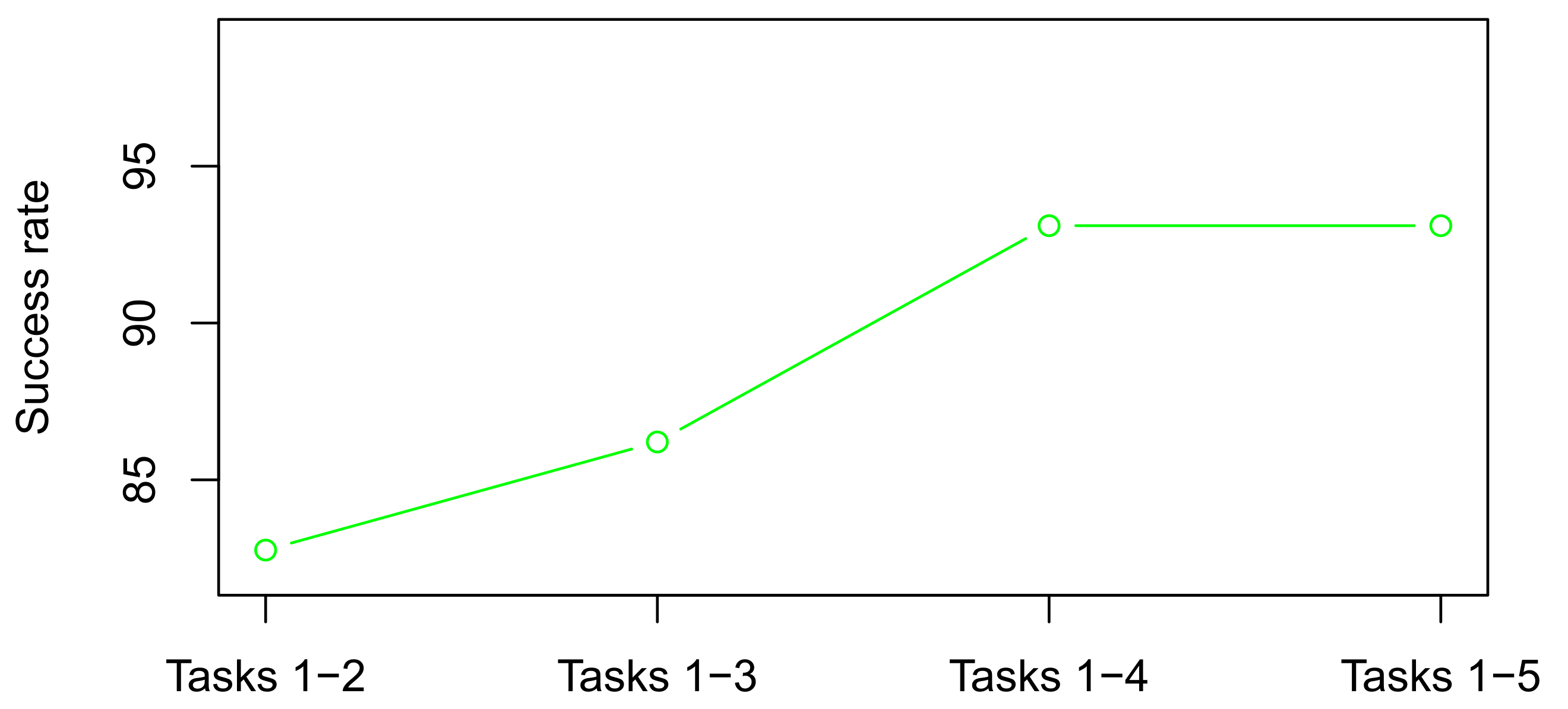
We have reported above the absolute misclassifications when predicting the test data making use of a model that is based on just Tasks 1 and 2 (research problem 1) to a model based on Tasks 1, 2, 3, 4, and 5 (research problem 4). All these misclassifications are summarized in Table 2 where we report the relative success rate of the procedure under the different studied scenarios. There, we can observe that, when applying to the test data the model that only makes use of Tasks 1 and 2 (research problem 1), we are able to predict the interval to which the average grade over the six Tasks belongs with a success rate of the 82.76%. This rate increases to the 86.21% when also making use of Task 3 (research problem 2) and stabilizes to the 93.10% success rate when making use of Tasks 1, 2, 3, and 4 (research problem 3). A display of these success rates is in Figure 4 where a rapid increase and stabilization of the success rates is observed. It is worth saying that we have been conservative in computing these success rates, considering as successful the entries in blue in Table 1 although, as explained above, there are other entries that could also be considered successful.
The obtained results are extremely good as after the student has completed just the two first tasks, we can predict their average final grade over the six tasks with a success rate of over the 80%; when completing the first three tasks with a success rate over the 85% and when completing the first four tasks with a success rate of over the 90%.
4. Discussion
The algorithm used is powerful in that it makes use of the random Tukey depth. This is due to two main reasons:
- 1.
- The random Tukey depth is computationally effective in reducing the dimension to one even if the original data dimension is high, as it happens with high dimensional or functional data [40].
- 2.
- The random Tukey depth behaves adequately [35] as it generally inherits the good properties of the Tukey depth, which is the most well-known in the literature but for it expensive computational time.
Furthermore, the kernel classifier performed on the resulting one-dimensional data is a well-known one but could be substituted by any other one-dimensional classifier. The only requirement being that the process can be automated as it occurs in this case.
Other works have carried out data-driven analysis of student academic activity with different objectives. Thus, ref [41] stores information on how students solve collaborative activities using CSCL systems and analyzed them to propose 17 strategies to optimize student performance. In other cases, the studies have focused on predicting the optimal number of students who should collaborate on the tasks [42]. Our study has a broader temporal scope. It is not about analyzing specific activities but rather predicting performance in an academic year.
The obtained results show a high success rate in predicting the average grade by just using the first two tasks performed by the students.
Thus, something that can be considered is the possibility of reducing the amount of tasks required of the students. Additionally, this would also allow an early intervention to improve the performance of the groups whose predicted grade is lower.
We can deduce that academic collaborative tasks imply greater richness and complexity due to the social interactions that take place, this work opens the door to consider the first tasks that students solve as predictive of academic performance in the rest of the course. The case study of this work illustrates how the method proposed can achieve this goal. This approach complements other works in the CSCL field that analyzes collaboration and interaction without predicting future academic performance [1,13,14]. However, our work has not delved into mechanisms that detail the causes (lack of communication, problems with the groupware system, etc.) that lead to an academic performance problem or in proposing automatic intervention strategies (adapting the groupware system, changing the composition of working groups, etc.).
5. Conclusions
This work has presented a proposal to automatically predict the academic performance of students using only the data recorded in the first tasks of the academic year. The interactions that students carry out with software tools to solve academic activities allow us to have datasets with which to try to carry out this prediction. In many active learning methodologies these activities are carried out collaboratively. For this reason, the work focused on experimenting with a real case in which the students collaborate in solving the tasks.
The proposal is based on a statistical depth based supervised classification technique, which first performs the random Tukey depth to lower to one the data dimension and then applies a kernel classifier. This means that the prediction can be carried out in an automated way, using support software that processes a significant amount of data. The experimentation carried out during four academic years in a university subject shows promising results, as just making use of the first two tasks that the students perform we obtain over an 80% success rate in predicting their final grade. This success rate increases to over the 90% success rate if the first four tasks, out of six, are known in predicting the final grade.
We propose that the results of the predictive mechanisms serve not only to inform what the academic performance of students would be at the end of the academic year but also to intervene in the automated development of activities. Our future work will address the analysis of the causes of task failures and to design intervention mechanisms in CSCL systems.
Author Contributions
Conceptualization, R.D.; methodology, A.N.-R.; validation, A.N.-R.; resources, R.D.; writing, A.N.-R., R.D. and G.F. All authors have read and agreed to the published version of the manuscript.
Funding
For A.N.-R., this research was funded by grant number MTM2017-86061-C2-2-P of the Spanish Ministry of Economy, Industry and Competitiveness. For R.D. this work was funded by the University of Cantabria through the teaching innovation project “Implantación de la técnica focus group para diseñar interfaces de usuario en la asignatura Interacción Persona-Computador” and “Utilización de las TIC para monitorizar y gestionar actividades colaborativas orientadas a resolver tareas de programación de algoritmos en el Grado en Ingeniería Informática.”
Institutional Review Board Statement
Not applicable.
Informed Consent Statement
This study does not involve personal information. Grades have been treated confidentially according to the regulations of the University of Cantabria.
Conflicts of Interest
The authors declare no conflict of interest.
Abbreviations
The following abbreviations are used in this manuscript:
| CSCL | Computer-Supported Cooperative Learning |
| HCI | Human-computer interaction |
| HTML | HyperText Markup Language |
| i.i.d. | independent and identically distributed |
| PBL | Project-Based Learning |
| WIMP | Windows Icon Menu Pointer |
References
- Duque, R.; Bollen, L.; Anjewierden, A.; Bravo, C. Automating the Analysis of Problem-solving Activities in Learning Environments: The Co-Lab Case Study. J. Univ. Comput. Sci. 2012, 18, 1279–1307. [Google Scholar]
- Kutlu, B.; Aggul, Y.G.; Atasu, I.; Kaymaz, Z. A Meta-Analysis of Studies on Groupware for Collaborative Work Environments. Proceedings 2021, 74, 9. [Google Scholar] [CrossRef]
- Dennis, A.R.; Carte, T.A.; Kelly, G.G. Breaking the rules: Success and failure in groupware-supported business process reengineering. Decis. Support Syst. 2003, 36, 31–47. [Google Scholar] [CrossRef] [Green Version]
- Duque, R.; Gómez-Pérez, D.; Nieto-Reyes, A.; Bravo, C. Analyzing collaboration and interaction in learning environments to form learner groups. Comput. Hum. Behav. 2015, 47, 42–49. [Google Scholar] [CrossRef] [Green Version]
- Bravo, C.; Redondo, M.A.; Verdejo, M.F.; Ortega, M. A framework for process–solution analysis in collaborative learning environments. Int. J. Hum. Comput. Stud. 2008, 66, 812–832. [Google Scholar] [CrossRef] [Green Version]
- Anderson, J.R.; Boyle, C.; Corbett, A.T.; Lewis, M.W. Cognitive modeling and intelligent tutoring. Artif. Intell. 1990, 42, 7–49. [Google Scholar] [CrossRef]
- Selker, T. COACH: A Teaching Agent That Learns. Commun. ACM 1994, 37, 92–99. [Google Scholar] [CrossRef]
- Paolucci, M.; Suthers, D.; Weiner, A. Automated advice-giving strategies for scientific inquiry. In Intelligent Tutoring Systems; Frasson, C., Gauthier, G., Lesgold, A., Eds.; Springer: Berlin/Heidelberg, Germany, 1996; pp. 372–381. [Google Scholar]
- Mørch, A.; Jondahl, S.; Dolonen, J. Supporting Conceptual Awareness with Pedagogical Agents. Inf. Syst. Front. 2005, 7, 39–53. [Google Scholar] [CrossRef] [Green Version]
- Du Boulay, B. Artificial Intelligence as an Effective Classroom Assistant. IEEE Intell. Syst. 2016, 31, 76–81. [Google Scholar] [CrossRef]
- Goel, A.K.; Polepeddi, L. Jill Watson: A Virtual Teaching Assistant for Online Education. In Learning Engineering for Online Education: Theoretical Contexts and Design-Based Examples; Routledge: New York, NY, USA, 2018. [Google Scholar]
- Uskola Ibarluzea, A.; Madariaga Orbea, J.M.; Arribillaga Iriarte, A.; Maguregi González, G.; Fernández Alonso, L. Categorisation of the Interventions of Faciliting Tutors on PBL and Their Relationship with Students’ Response. Profr.: Rev. Curric. Form. Profr. 2018, 22, 153–170. [Google Scholar] [CrossRef]
- Splichal, J.M.; Oshima, J.; Oshima, R. Regulation of collaboration in project-based learning mediated by CSCL scripting reflection. Comput. Educ. 2018, 125, 132–145. [Google Scholar] [CrossRef]
- Chen, L.; Chen, P.; Lin, Z. Artificial Intelligence in Education: A Review. IEEE Access 2020, 8, 75264–75278. [Google Scholar] [CrossRef]
- Li, Z.; Hoiem, D. Learning without Forgetting. IEEE Trans. Pattern Anal. Mach. Intell. 2018, 40, 2935–2947. [Google Scholar] [CrossRef] [Green Version]
- Aljundi, R.; Chakravarty, P.; Tuytelaars, T. Expert Gate: Lifelong Learning with a Network of Experts. In Proceedings of the 2017 IEEE Conference on Computer Vision and Pattern Recognition (CVPR), Honolulu, HI, USA, 21–26 July 2017; pp. 7120–7129. [Google Scholar] [CrossRef] [Green Version]
- Phielix, C.; Prins, F.J.; Kirschner, P.A. The Design of Peer Feedback and Reflection Tools in a CSCL Environment. In Proceedings of the 9th International Conference on Computer Supported Collaborative Learning, Rhodes, Greece, 8–13 June 2009; Volume 1, pp. 626–635. [Google Scholar]
- Zuo, Y.; Serfling, R. General notions of statistical depth function. Ann. Statist. 2000, 28, 461–482. [Google Scholar] [CrossRef]
- Härdle, W. Applied Nonparametric Regression; Econometric Society Monographs, Cambridge University Press: Cambridge, UK, 1990. [Google Scholar] [CrossRef]
- Gerosa, M.A.; Pimentel, M.; Fuks, H.; de Lucena, C.J.P. Development of Groupware Based on the 3C Collaboration Model and Component Technology. In Groupware: Design, Implementation, and Use; Dimitriadis, Y.A., Zigurs, I., Gómez-Sánchez, E., Eds.; Springer: Berlin/Heidelberg, Germany, 2006; pp. 302–309. [Google Scholar]
- Duque, R.; Bravo, C.; Ortega, M. A model-based framework to automate the analysis of users’ activity in collaborative systems. J. Netw. Comput. Appl. 2011, 34, 1200–1209. [Google Scholar] [CrossRef]
- Cuesta-Albertos, J.A.; Nieto-Reyes, A. The random Tukey depth. Comput. Statist. Data Anal. 2008, 52, 4979–4988. [Google Scholar] [CrossRef]
- Zuo, Y. On General Notions of Depth for Regression. Stat. Sci. 2021, 36, 142–157. [Google Scholar] [CrossRef]
- Nieto-Reyes, A.; Battey, H. A Topologically Valid Definition of Depth for Functional Data. Stat. Sci. 2016, 31, 61–79. [Google Scholar] [CrossRef]
- Nieto-Reyes, A.; Battey, H. A topologically valid construction of depth for functional data. J. Multivar. Anal. 2021, 184, 104738. [Google Scholar] [CrossRef]
- Nieto-Reyes, A.; Battey, H.; Francisci, G. Functional Symmetry and Statistical Depth for the Analysis of Movement Patterns in Alzheimer’s Patients. Mathematics 2021, 9, 820. [Google Scholar] [CrossRef]
- Saraceno, G.; Agostinelli, C. Robust multivariate estimation based on statistical depth filters. TEST 2021, 1–25. [Google Scholar] [CrossRef]
- Pandolfo, G.; Iorio, C.; Staiano, M.; Aria, M.; Siciliano, R. Multivariate process control charts based on the Lp depth. Appl. Stoch. Model. Bus. Ind. 2007, 37, 229–250. [Google Scholar] [CrossRef]
- Liu, R.Y. On a notion of data depth based on random simplices. Ann. Statist. 1990, 18, 405–414. [Google Scholar] [CrossRef]
- Serfling, R. A depth function and a scale curve based on spatial quantiles. In Statistical Data Analysis Based on the L1-norm and Related Methods (Neuchâtel, 2002); Stat. Ind. Technol.: Basel, Switzerland, 2002; pp. 25–38. [Google Scholar]
- Liu, R.Y.; Serfling, R.; Souvaine, D.L. (Eds.) Data Depth: Robust Multivariate Analysis, Computational Geometry and Applications; DIMACS Series in Discrete Mathematics and Theoretical Computer Science, 72; American Mathematical Society: Providence, RI, USA, 2006; p. xiv+246. [Google Scholar]
- Liu, Z.; Modarres, R. Lens data depth and median. J. Nonparametric Stat. 2011, 23, 1063–1074. [Google Scholar] [CrossRef]
- Tukey, J.W. Mathematics and the picturing of data. In Proceedings of the International Congress of Mathematicians (Vancouver, B. C., 1974), Vancouver, Canada, 21–29 August 1974; Canadian Mathematical Congress. 1975; Volume 2, pp. 523–531. Available online: https://www.mathunion.org/fileadmin/ICM/Proceedings/ICM1974.2/ICM1974.2.ocr.pdf (accessed on 20 October 2021).
- Dyckerhoff, R.; Mozharovskyi, P. Exact computation of the halfspace depth. Comput. Stat. Data Anal. 2016, 98, 19–30. [Google Scholar] [CrossRef] [Green Version]
- Cuesta-Albertos, J.; Nieto-Reyes, A. The Tukey and the random Tukey depths characterize discrete distributions. J. Multivar. Anal. 2008, 99, 2304–2311. [Google Scholar] [CrossRef] [Green Version]
- Ferraty, F.; Vieu, P. Nonparametric Functional Data Analysis: Theory and Practice (Springer Series in Statistics); Springer: Berlin/Heidelberg, Germany, 2006. [Google Scholar]
- Ferraty, F.; Vieu, P. Curves discrimination: A nonparametric functional approach. Comput. Stat. Data Anal. 2003, 44, 161–173. [Google Scholar] [CrossRef]
- Nadaraya, E.A. On estimating regression. Theory Probab. Appl. 1964, 9, 141–142. [Google Scholar] [CrossRef]
- Watson, G.S. Smooth regression analysis. Sankhyā Ser. 1964, 26, 359–372. [Google Scholar]
- Cuesta-Albertos, J.A.; Nieto-Reyes, A. Functional Classification and the Random Tukey Depth. Practical Issues. In Combining Soft Computing and Statistical Methods in Data Analysis; Borgelt, C., González-Rodríguez, G., Trutschnig, W., Lubiano, M.A., Gil, M.Á., Grzegorzewski, P., Hryniewicz, O., Eds.; Springer: Berlin/Heidelberg, Germany, 2010; pp. 123–130. [Google Scholar]
- Zheng, L. Optimize CSCL Activities Based on a Data-Driven Approach. In Data-Driven Design for Computer-Supported Collaborative Learning: Design Matters; Springer: Singapore, 2021; pp. 147–162. [Google Scholar] [CrossRef]
- Omae, Y.; Furuya, T.; Mizukoshi, K.; Oshima, T.; Sakakibara, N.; Mizuochi, Y.; Yatsushiro, K.; Takahashi, H. Machine learning-based collaborative learning optimizer toward intelligent CSCL system. In Proceedings of the 2017 IEEE/SICE International Symposium on System Integration (SII), Taipei, Taiwan, 11–14 December 2017; pp. 577–582. [Google Scholar] [CrossRef]
Figure 1.
n is equal to ten and the random Tukey depth of x (left-hand side) and y (right-hand side) are, respectively, given, among others, by the randomly obtained closed halfspaces painted in pastel blue.Computing Tukey depth.
Figure 1.
n is equal to ten and the random Tukey depth of x (left-hand side) and y (right-hand side) are, respectively, given, among others, by the randomly obtained closed halfspaces painted in pastel blue.Computing Tukey depth.

Figure 2.
Outline of the process followed to experiment with the methodology.

Figure 3.
Illustration of the grades of the different groups in the academic periods 2017/18 (black), 2018/19 (red), 2019/20 (green) and 2020/21 (blue). Grades of Tasks 1 and 2 in the left plot, of Tasks 3 and 4 in the central plot and of Tasks 5 and 6 in the right plot. Each group in an academic period is labeled by a corresponding number.

Figure 4.
Display of the success rates in Table 2. The OX-axis shows the tasks used in the model to predict the interval of the average grade; it goes from Tasks 1 and 2 (research problem 1) in the left corner of the axis to Tasks 1, 2, 3, 4, and 5 (research problem 4) in the right corner.
Figure 4.
Display of the success rates in Table 2. The OX-axis shows the tasks used in the model to predict the interval of the average grade; it goes from Tasks 1 and 2 (research problem 1) in the left corner of the axis to Tasks 1, 2, 3, 4, and 5 (research problem 4) in the right corner.


Table 1.
Four confusion matrices between the real average grade intervals (columns) and the estimated average grade intervals (rows) for the test data (academic course 2020/21) on the model constructed using the training data (academic courses 2017/18, 2018/19, 2019/20). 3 test data belong to the interval [0,4), 4 to [7,8), 13 to [8,9), and 9 to [9,10) (intervals reported in (6)). The analysis is based on: Tasks 1 and 2 (top matrix), Tasks 1, 2 and 3 (second matrix from the top), Tasks 1, 2, 3, and 4 (third matrix from the top) and Tasks 1, 2, 3, 4, and 5 (bottom matrix). The average grades make use of the six Tasks. The groups of students whose average grade is clearly correctly classified are in blue. The omitted values correspond to zeros.
| TEST SAMPLE | ||||||
|---|---|---|---|---|---|---|
| Tasks 1–2 (research problem 1) | ||||||
| estimated | ||||||
| [0,4] | [5,7] | [6,8] | [7,9] | [8,10] | ||
| [0,4) | 3 | |||||
| real | [7,8) | 4 | ||||
| [8,9) | 3 | 10 | ||||
| [9,10) | 1 | 1 | 7 | |||
| Tasks 1–3 (research problem 2) | ||||||
| estimated | ||||||
| [0,4] | [5,7] | [6,8] | [7,9] | [8,10] | ||
| [0,4) | 2 | 1 | ||||
| real | [7,8) | 1 | 3 | |||
| [8,9) | 13 | |||||
| [9,10) | 2 | 7 | ||||
| Tasks 1–4 (research problem 3) | ||||||
| estimated | ||||||
| [0,4] | [5,7] | [6,8] | [7,9] | [8,10] | ||
| [0,4) | 1 | 2 | ||||
| real | [7,8) | 4 | ||||
| [8,9) | 13 | |||||
| [9,10) | 9 | |||||
| Tasks 1–5 (research problem 4) | ||||||
| estimated | ||||||
| [0,4] | [5,7] | [6,8] | [7,9] | [8,10] | ||
| [0,4) | 1 | 2 | ||||
| real | [7,8) | 4 | ||||
| [8,9) | 13 | |||||
| [9,10) | 9 | |||||
Table 2.
Success rates for the supervised classification of average grade intervals over 6 tasks for the test data on the model constructed using the training data. Test data refer to the groups in the academic course 2020/21 and training data to the groups along the academic courses 2017/18, 2018/19, and 2019/20. The analysis is based on: Tasks 1 and 2 (left column), Tasks 1, 2, and 3 (second left column), Tasks 1, 2, 3, and 4 (third left column) and Tasks 1, 2, 3, 4, and 5 (right column). For the success rate, it is used as correctly classified only the groups of students whose average grade is displayed in blue in Table 1.
| Tasks 1–2 (Research Problem 1) | Tasks 1–3 (Research Problem 2) | Tasks 1–4 (Research Problem 3) | Tasks 1–5 (Research Problem 4) | |
|---|---|---|---|---|
| Test | 82.76% | 86.21% | 93.10% | 93.10% |
Publisher’s Note: MDPI stays neutral with regard to jurisdictional claims in published maps and institutional affiliations. |
© 2021 by the authors. Licensee MDPI, Basel, Switzerland. This article is an open access article distributed under the terms and conditions of the Creative Commons Attribution (CC BY) license (https://creativecommons.org/licenses/by/4.0/).
Share and Cite
MDPI and ACS Style
Nieto-Reyes, A.; Duque, R.; Francisci, G. A Method to Automate the Prediction of Student Academic Performance from Early Stages of the Course. Mathematics 2021, 9, 2677. https://0-doi-org.brum.beds.ac.uk/10.3390/math9212677
AMA Style
Nieto-Reyes A, Duque R, Francisci G. A Method to Automate the Prediction of Student Academic Performance from Early Stages of the Course. Mathematics. 2021; 9(21):2677. https://0-doi-org.brum.beds.ac.uk/10.3390/math9212677
Chicago/Turabian StyleNieto-Reyes, Alicia, Rafael Duque, and Giacomo Francisci. 2021. "A Method to Automate the Prediction of Student Academic Performance from Early Stages of the Course" Mathematics 9, no. 21: 2677. https://0-doi-org.brum.beds.ac.uk/10.3390/math9212677
Note that from the first issue of 2016, this journal uses article numbers instead of page numbers. See further details here.