Synchronizability of Multi-Layer Variable Coupling Windmill-Type Networks

Abstract

The system model on synchronizability problem of complex networks with multi-layer structure is closer to the real network than the usual single-layer case. Based on the master stability equation (MSF), this paper studies the eigenvalue spectrum of two k-layer variable coupling windmill-type networks. In the case of bounded and unbounded synchronization domain, the relationships between the synchronizability of the layered windmill-type networks and network parameters, such as the numbers of nodes and layers, inter-layers coupling strength, are studied. The simulation of the synchronizability of the layered windmill-type networks are given, and they verify the theoretical results well. Finally, the optimization schemes of the synchronizability are given from the perspective of single-layer and multi-layer networks, and it was found that the synchronizability of the layered windmill-type networks can be improved by changing the parameters appropriately.

1. Introduction

Complex network is a significant interdisciplinary research field that has raised the wide attention of both scientists and engineers. The most common complex networks in nature include neural networks, financial networks, group flight networks of birds, social networks, etc. In the past decades, much progress has been made in many aspects related with complex networks, such as the synchronization of multi-layer networks [1,2,3,4,5,6,7,8,9,10], consensus problems [11,12], diffusion dynamics [13,14,15,16], robustness and spectral properties of complex networks [17,18,19,20].

The synchronization problem is a significant research topic of complex networks that are often related with phenomena in the real world, such as applause synchronization during performance, simultaneous flicker of fireflies and UAV formation synchronization, and the synchronization-related problems are also an interdisciplinary research topic which may include physics, biology, engineering technology and social science, etc. There exist lots of good research works on the synchronization of the usual single-layer networks, and the results of multi-layer networks that are closer to the actual situation [21,22,23] are relatively few. Li et al. [21] compared the size relationships of the synchronizability of two kinds of double-layer dumbbell networks under different coupling modes between layers when the synchronization domain is bounded and unbounded, and verified that the coupling between key nodes between layers has a significant impact on the synchronizability of double-layer dumbbell networks. Zhang et al. [22] gave the analytical expression of the supra-Laplacian matrix of multi-layer K-neighbor networks and analyzed the influence of various parameters on the synchronizability of multi-layer K-neighbor networks in the case of unbounded and bounded synchronization domain. Wang et al. [23] studied the synchronization of multi-layer fully coupled networks and analyzed the key factors affecting the synchronizability. It was proven that multi-layer fully coupled networks have the same synchronizability as the corresponding simplest equivalent networks. The main contributions of this paper are as follows:

• Two sorts of novel multi-layered windmill-type networks with different connection relations among the leader nodes are proposed.
• According to the real situation, the networks of various coupling strengths are considered, and the relationships between the network synchronizability and various parameters of the two windmill-type networks are studied in the case of bounded and unbounded synchronization domain.
• Under the same initial conditions, the network synchronizability of the two sorts of layered windmill-type networks are compared, which provides a practical optimization scheme to improve the synchronizability.

The paper is organized as follows: The preliminaries for the study of windmill-type networks are given in Section 2. The weighted Laplacian spectrum and synchronizability index of variable coupling windmill-type $G_1^K(m,n,k)$ are studied in Section 3. The spectrum and synchronizability index of variable coupling windmill-type $G_2^K(m,n,k)$ are obtained in Section 4. The synchronizabilities of the windmill-type networks are simulated and analyzed in Section 5. The conclusion is given in Section 6.

2. Preliminaries

2.1. Dynamics Model of the Networks

The dynamics of the ith node of the $Mth$ layer in a K layer network is:

$${\dot{x}}_i^M=f\left(x_i^M\right)-a_M\sum _{\genfrac{}{}{0pt}{}{j=1}{}}^N{l}_{ij}^{M}H\left(x_j^M\right)-d_{ML}\sum _{\genfrac{}{}{0pt}{}{L=1}{}}^K{d}_i^{ML}\Gamma \left(x_i^L\right),$$

(1)

$$i=1,2,\cdots ,N;M=1,2,\cdots ,K.$$

where $x_i^M\in {\mathbb{R}}^{\mathbb{N}}$ represents the state of the ith node of the $Mth$ layer, $f(*)$ represents the dynamic function, H is the intra-layer coupling function and $\Gamma$ is the inter-layer coupling function. $a_M$ represents the intra-layer coupling strength of the $Mth$ layer, and $d_{ML}$ represents the inter-layer coupling strength between the $Mth$ layer and the $Lth$ layer. $L^M=\left(l_{ij}^M\right)\in R^{N\times N}$ is the Laplacian matrix of the $Mth$ layer. $L^M=S^M-W^M$, here, $S^M=\left(s_{ij}^M\right)$ is the degree matrix of the $Mth$ layer, $s_{ij}^M=0(i\ne j),s_{ii}^M=d\left(v_i\right)$, $d\left(v_i\right)$ is the degree of node $v_i$, $W^M=\left(w_{ij}^M\right)$ is the adjacency matrix of the $Mth$ layer, if the nodes $v_i$ and $v_j$ are adjacent in the $Mth$ layer, $w_{ij}^M=1$, otherwise $w_{ij}^M=0$. $D=\left(d_i^{ML}\right)\in {\mathbb{R}}^{\mathbb{K}\times \mathbb{K}}$ is the inter-layer coupling matrix, if there is an edge between the $ith$ node of the $Mth$ layer and the $ith$ node of the $Lth$ layer, $d_i^{ML}=-1$, otherwise, $d_i^{ML}=0,d_i^{MM}=-{\sum }_{\genfrac{}{}{0pt}{}{L=1}{L\ne M}}^K{d}_i^{ML},L,M=1,2,\cdots ,K.$

(1) can be written as a vector in the form

$$\dot{x}=F\left(x\right)-({\Lambda }^L\otimes H)x-({\Lambda }^I\otimes \Gamma )x,$$

(2)

where ⊗ is the Kronecker product, $x=(x^1,x^2,\cdots ,x^N)$, $F\left(x\right)=(f\left(x^1\right),f\left(x^2\right),\cdots ,f\left(x^N\right))$.

Let ${\Lambda }^L$ be the supra-Laplacian matrix of the intra-layer and ${\Lambda }^I$ be the supra-Laplacian matrix of the inter-layer. The supra-Laplacian matrix of model (1) can be written as $\Lambda ={\Lambda }^L+{\Lambda }^I$. Here,

$${\Lambda }^L=\left(\begin{array}{cccc}{a}_1{L}^{\left(1\right)}& 0& \cdots & 0\\ 0& a_2{L}^{\left(2\right)}& \cdots & 0\\ ⋮& ⋮& \ddots & ⋮\\ 0& 0& \cdots & a_K{L}^{\left(K\right)}\end{array}\right),$$

(3)

${\Lambda }^I=dD\otimes I_N$, where $I_N$ is the identity matrix of $N\times N$.

2.2. Measurement Method of the Multi-Layer Network Synchronizability

The synchronizability of multi-layer networks are determined by the eigenvalue spectrum of the supra-Laplacian matrix $\Lambda$. The supra-Laplacian matrix $\Lambda$ has a zero eigenvalue with multiplicity 1, and the other eigenvalues are positive real numbers. It can be assumed that $0={\lambda }_1<{\lambda }_2\le {\lambda }_3\le \cdots \le {\lambda }_{max}$.

The synchronizability of multi-layer networks are closely related to the synchronization domain $SR$. According to the master stability function theory, the synchronization domain is divided into the following four cases:

• The synchronous region is bounded. $SR=({\alpha }_1,{\alpha }_2)$, c is the coupling strength of the network, then ${\alpha }_1<c{\lambda }_k<{\alpha }_2$, $r={\lambda }_{max}/{\lambda }_2<{\alpha }_2/{\alpha }_1$; the smaller the ratio r of the maximum eigenvalue to the minimum non-zero eigenvalue of the Laplacian matrix, the stronger the synchronizability of the network.
• The synchronous region is unbounded. $SR=({\alpha }_1,+\infty )$, then ${\alpha }_1<c{\lambda }_2\le c{\lambda }_3\le \cdots c{\lambda }_{max}$, ${\alpha }_1<c{\lambda }_2$; the larger the minimum non-zero eigenvalue ${\lambda }_2$ of the Laplacian matrix, the stronger the synchronizability of the network.
• The synchronous region is the union of several unconnected regions. Duan [24] found it is difficult to realize the synchronizability.
• When the synchronous region is an empty set, it can not achieve the complete synchronizability no matter how the topology and coupling strength change.

Through the above analysis, two important indicators describing the synchronizability of complex networks are obtained: (I) if the synchronization region is unbounded, then the larger the minimum non-zero eigenvalue ${\lambda }_2$ of the Laplacian matrix, the stronger the synchronizability of the network; (II) if the synchronization region is bounded, then the smaller the ratio r is, the stronger the synchronizability of the network.

2.3. Two Multi-Layer Windmill-Type Networks

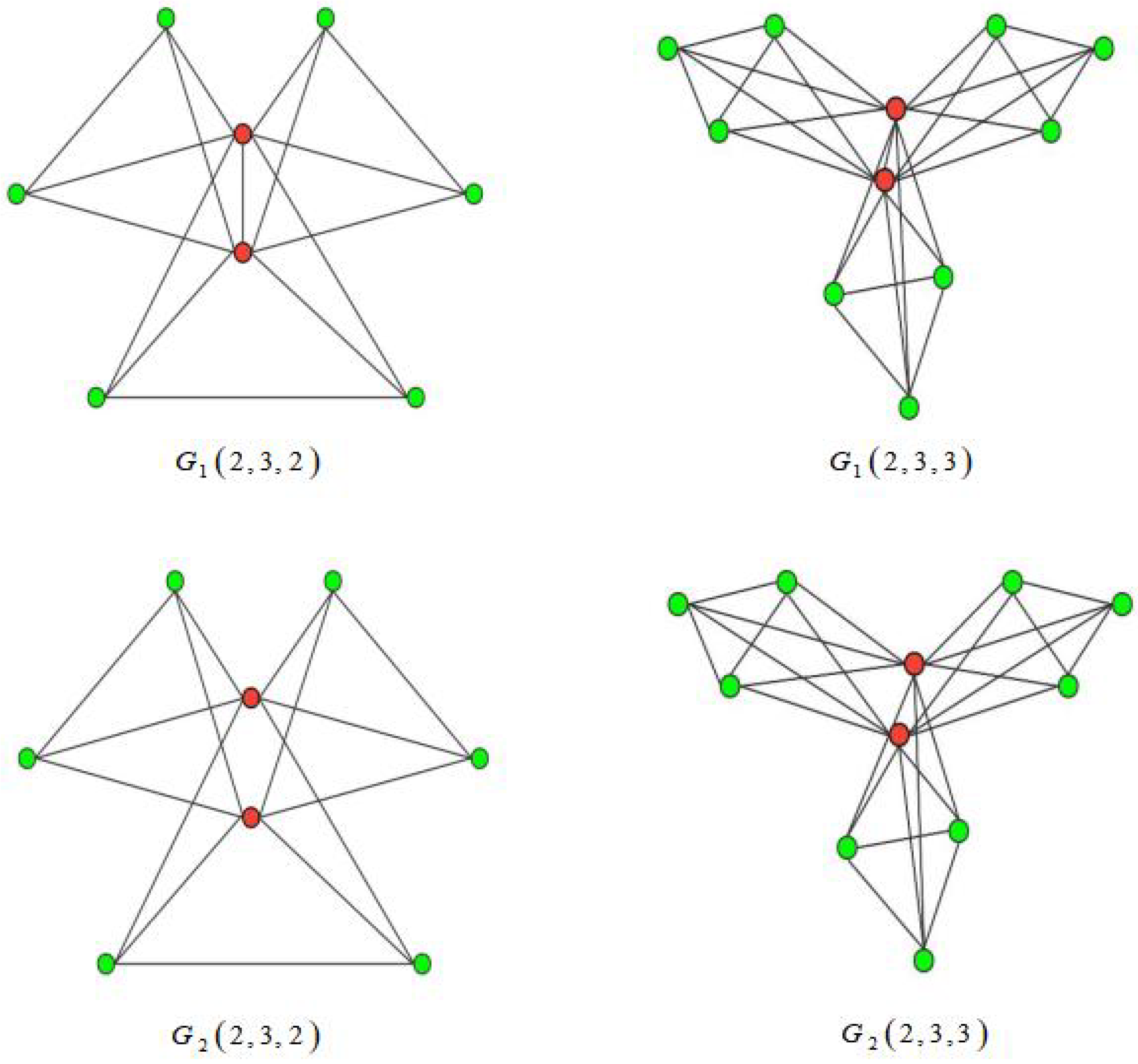
Kooij, W. Sun [25,26] proposed generalized windmill-type graphs $G_1(m,n,k)$ and $G_2(m,n,k)$. $G_1(m,n,k)$ is made up of m center nodes and n groups of complete graphs $K_k$. Each node of $K_k$ is connected to m center nodes, and the center nodes constitute a complete graph $K_m$. The difference between $G_2(m,n,k)$ and $G_1(m,n,k)$ is that the center nodes of $G_2(m,n,k)$ are disconnected with each other. The graph structures are shown in Figure 1.

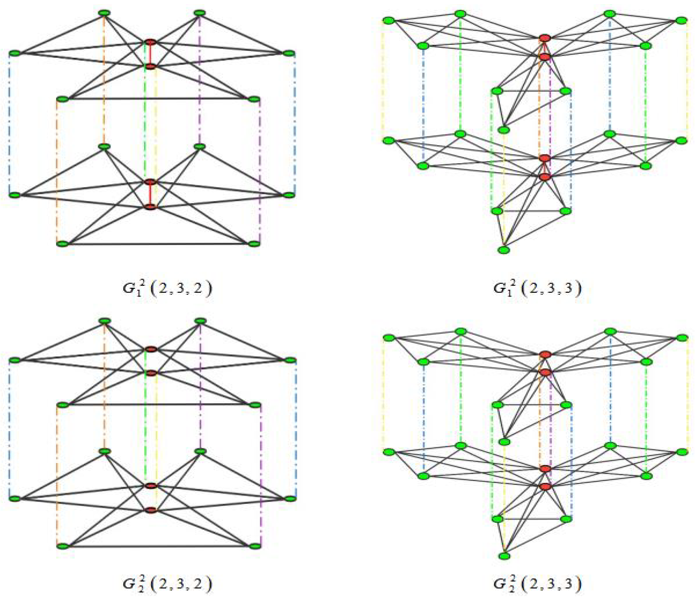
In recent years, scholars have found that the practical significance of multi-layer networks is closer to real applications than the normal single-layer one [27,28]. The single-layer windmill-type networks are extended to multi-layer structures in our research. $G_1^K(m,n,k),G_2^K(m,n,k)$ is formed by $G_1(m,n,k),G_2(m,n,k)$ combination superposition K times; K denotes the number of network layers; the total number of nodes are $K(m+nk)$; and their connection relationships are shown in Figure 2. The red nodes represent the leader nodes, the green nodes represent the follower nodes, and the black solid lines represent the inter-layer connection relationships between nodes. The colored dotted lines represent the connection relationships between node layers, in which the networks structure of each layer are the same.

Lemma 1

([7]). Let A and B be two $L\times L$ square matrices, Z be an integer. Then

$${\left|\begin{array}{cccc}A& B& \cdots & B\\ B& A& \cdots & B\\ ⋮& ⋮& \ddots & ⋮\\ B& B& \cdots & A\end{array}\right|}_{Z\times Z}={|A+(Z-1)B|·|A-B|}^{(Z-1)}$$

3. The Eigenvalue Spectrum and Synchronizability Index of ${\mathit{G}}_{\mathit{1}}^{\mathit{K}}(\mathit{m},\mathit{n},\mathit{k})$

Note that d is the inter-layer coupling strength, ${\omega }_0$ is the coupling strength among the leader nodes in the layers, ${\omega }_1$ is the coupling strength between the leader nodes and the follower nodes in the same layer, ${\omega }_2$ is the coupling strength between the follower nodes in the layers. According to the practical application in life, it may be assumed that ${\omega }_0\ge {\omega }_1\ge {\omega }_2,nk\ge m$. Next, we discuss the spectrum of $G_1^K(m,n,k)$.

$$L_1={\left(\begin{array}{ccccc}{\Omega }_1& -{\omega }_0& -{\omega }_0& \cdots & -{\omega }_0\\ -{\omega }_0& {\Omega }_1& -{\omega }_0& \cdots & -{\omega }_0\\ -{\omega }_0& -{\omega }_0& {\Omega }_1& \cdots & -{\omega }_0\\ ⋮& ⋮& ⋮& \ddots & ⋮\\ -{\omega }_0& -{\omega }_0& -{\omega }_0& \cdots & {\Omega }_1\end{array}\right)}_{m\times m},$$

$$L_2={\left(\begin{array}{ccccc}-{\omega }_1& -{\omega }_1& -{\omega }_1& \cdots & -{\omega }_1\\ -{\omega }_1& -{\omega }_1& -{\omega }_1& \cdots & -{\omega }_1\\ -{\omega }_1& -{\omega }_1& -{\omega }_1& \cdots & -{\omega }_1\\ ⋮& ⋮& ⋮& \ddots & ⋮\\ -{\omega }_1& -{\omega }_1& -{\omega }_1& \cdots & -{\omega }_1\end{array}\right)}_{m\times k},$$

$$L_3={\left(\begin{array}{ccccc}{\Omega }_2& -{\omega }_2& -{\omega }_2& \cdots & -{\omega }_0\\ -{\omega }_2& {\Omega }_2& -{\omega }_2& \cdots & -{\omega }_2\\ -{\omega }_2& -{\omega }_2& {\Omega }_2& \cdots & -{\omega }_2\\ ⋮& ⋮& ⋮& \ddots & ⋮\\ -{\omega }_2& -{\omega }_2& -{\omega }_2& \cdots & {\Omega }_2\end{array}\right)}_{k\times k},$$

where ${\Omega }_1=(m-1){\omega }_0+nk{\omega }_1$ and ${\Omega }_2=m{\omega }_1+(k-1){\omega }_2$.

The supra-Laplacian matrix in each layer is

$$a{L}^I={\left(\begin{array}{ccccc}{L}_1& L_2& L_2& \cdots & L_2\\ L_2^T& L_3& 0& \cdots & 0\\ L_2^T& 0& L_3& \cdots & 0\\ ⋮& ⋮& ⋮& \ddots & ⋮\\ L_2^T& 0& 0& \cdots & L_3\end{array}\right)}_{(m+nk)\times (m+nk)},$$

combined with the inter-layer supra-Laplacian matrix, we have

$${\Lambda }_1=\left(\begin{array}{ccccc}{\Omega }_3& -dI& \cdots & -dI& -dI\\ -dI& {\Omega }_3& \cdots & -dI& -dI\\ ⋮& ⋮& ⋮& ⋮& ⋮\\ -dI& -dI& \cdots & {\Omega }_3& -dI\\ -dI& -dI& \cdots & -dI& {\Omega }_3\end{array}\right).$$

$${\Phi }_I\left(\lambda \right)=det(\lambda I-{\Lambda }_1)=\left|\begin{array}{ccccc}{\Omega }_4& dI& \cdots & dI& dI\\ dI& {\Omega }_4& \cdots & dI& dI\\ ⋮& ⋮& ⋮& ⋮& ⋮\\ dI& dI& \cdots & {\Omega }_4\\ dI& dI& \cdots & dI& {\Omega }_4\end{array}\right|,$$

(4)

where ${\Omega }_3=a{L}^I+(K-1)dI$ and ${\Omega }_4=\lambda I-a{L}^I-(K-1)dI$.

According to Lemma 1,

$${\Phi }_I\left(\lambda \right)=|\lambda I-a{L}^I\left|\right|\lambda I-a{L}^I{-KdI|}^{K-1},$$

$$L_4={\left(\begin{array}{ccccc}{\Omega }_5& {\omega }_2-{\omega }_1& {\omega }_2-{\omega }_1& \cdots & {\omega }_2-{\omega }_1\\ {\omega }_2-{\omega }_1& {\Omega }_5& {\omega }_2-{\omega }_1& \cdots & {\omega }_2-{\omega }_1\\ {\omega }_2-{\omega }_1& {\omega }_2-{\omega }_1& {\Omega }_5& \cdots & {\omega }_2-{\omega }_1\\ ⋮& ⋮& ⋮& \ddots & ⋮\\ {\omega }_2-{\omega }_1& {\omega }_2-{\omega }_1& {\omega }_2-{\omega }_1& \cdots & {\Omega }_5\end{array}\right)}_{k\times k},$$

where ${\Omega }_5=\lambda -(m+1){\omega }_1-(k-1){\omega }_2$.

$$L_5={\left(\begin{array}{ccccc}-{\omega }_1& -{\omega }_1& -{\omega }_1& \cdots & -{\omega }_1\\ -{\omega }_1& -{\omega }_1& -{\omega }_1& \cdots & -{\omega }_1\\ -{\omega }_1& -{\omega }_1& -{\omega }_1& \cdots & -{\omega }_1\\ ⋮& ⋮& ⋮& \ddots & ⋮\\ -{\omega }_1& -{\omega }_1& -{\omega }_1& \cdots & -{\omega }_1\end{array}\right)}_{k\times k}.$$

$$\begin{array}{cc}& |\lambda I-a{L}^I|\hfill \\ \hfill =& \lambda {(\lambda -m{\omega }_0-nk{\omega }_1)}^{m-1}\left|\begin{array}{cccc}{L}_4& L_5& \cdots & L_5\\ L_5& L_4& \cdots & L_5\\ ⋮& ⋮& \ddots & ⋮\\ L_5& L_5& \cdots & L_4\end{array}\right|\hfill \\ \hfill =& \lambda {(\lambda -m{\omega }_0-nk{\omega }_1)}^{m-1}(\lambda -m{\omega }_1-nk{\omega }_1){(\lambda -m{\omega }_1)}^{n-1}{(\lambda -m{\omega }_1-k{\omega }_2)}^{n(k-1)}.\hfill \end{array}$$

(5)

The eigenvalue spectrum of ${\Lambda }_1$ are

$$\begin{array}{c}0,\underset{m-1}{\underbrace{m{\omega }_0+nk{\omega }_1}},(m+nk){\omega }_1,\underset{n-1}{\underbrace{m{\omega }_1}},\underset{n(k-1)}{\underbrace{m{\omega }_1+k{\omega }_2}}\\ \underset{K-1}{\underbrace{Kd,\underset{m-1}{\underbrace{m{\omega }_0+nk{\omega }_1+Kd}},(m+nk){\omega }_1+Kd}}\\ \underset{K-1}{\underbrace{\underset{n-1}{\underbrace{m{\omega }_1+Kd}},\underset{n(k-1)}{\underbrace{m{\omega }_1+k{\omega }_2+Kd}}}}.\end{array}$$

(6)

In the case of ${\omega }_0\ge {\omega }_1\ge {\omega }_2,nk\ge m$, the minimum nonzero eigenvalue is ${\lambda }_2=min\{m{\omega }_1,Kd\}$. The maximum eigenvalue is ${\lambda }_{max}=m{\omega }_0+nk{\omega }_1+Kd$.

4. The Eigenvalue Spectrum and Synchronizability Index of ${\mathit{G}}_2^{\mathit{K}}(\mathit{m},\mathit{n},\mathit{k})$

Similar to the method of the eigenvalue spectrum calculated by $G_1^K(m,n,k)$, the eigenvalue spectrum of $G_2^K(m,n,k)$ can be derived as follows:

$$L_6={\left(\begin{array}{ccccc}nk{\omega }_1& 0& 0& \cdots & 0\\ 0& nk{\omega }_1& 0& \cdots & 0\\ 0& 0& nk{\omega }_1& \cdots & 0\\ ⋮& ⋮& ⋮& \ddots & ⋮\\ 0& 0& 0& \cdots & nk{\omega }_1\end{array}\right)}_{m\times m},$$

The supra-Laplacian matrix in each layer is

$$a{L}^{II}={\left(\begin{array}{ccccc}{L}_6& L_2& L_2& \cdots & L_2\\ L_2^T& L_3& 0& \cdots & 0\\ L_2^T& 0& L_3& \cdots & 0\\ ⋮& ⋮& ⋮& \ddots & ⋮\\ L_2^T& 0& 0& \cdots & L_3\end{array}\right)}_{(m+nk)\times (m+nk)},$$

combined with the inter-layer supra-Laplacian matrix, we have

$${\Lambda }_2=\left(\begin{array}{ccccc}{\Omega }_7& -dI& \cdots & -dI& -dI\\ -dI& {\Omega }_7& \cdots & -dI& -dI\\ ⋮& ⋮& ⋮& ⋮& ⋮\\ -dI& -dI& \cdots & {\Omega }_7& -dI\\ -dI& -dI& \cdots & -dI& {\Omega }_7\end{array}\right),$$

where ${\Omega }_7=a{L}^{II}+(K-1)dI$.

According to Lemma 1,

$${\Phi }_{II}\left(\lambda \right)=|\lambda I-a{L}^{II}\left|\right|\lambda I-a{L}^{II}{-KdI|}^{K-1}$$

(7)

Similar to the calculation in (5),

$$\begin{array}{c}|\lambda I-a{L}^{II}|=\lambda {(\lambda -nk{\omega }_1)}^{m-1}\left|\begin{array}{cccc}{L}_4& L_5& \cdots & L_5\\ L_5& L_4& \cdots & L_5\\ ⋮& ⋮& \ddots & ⋮\\ L_5& L_5& \cdots & L_4\end{array}\right|\hfill \\ =\lambda {(\lambda -nk{\omega }_1)}^{m-1}(\lambda -m{\omega }_1-nk{\omega }_1){(\lambda -m{\omega }_1)}^{n-1}{(\lambda -m{\omega }_1-k{\omega }_2)}^{n(k-1)}.\hfill \end{array}$$

(8)

The eigenvalue spectrum of ${\Lambda }_2$ are

$$0,\underset{m-1}{\underbrace{nk{\omega }_1}},(m+nk){\omega }_1,\underset{n-1}{\underbrace{m{\omega }_1}},\underset{n(k-1)}{\underbrace{m{\omega }_1+k{\omega }_2}}$$

$$\underset{K-1}{\underbrace{Kd,\underset{m-1}{\underbrace{nk{\omega }_1+Kd}},(m+nk){\omega }_1+Kd}}.$$

$$\underset{K-1}{\underbrace{\underset{n-1}{\underbrace{m{\omega }_1+Kd}},\underset{n(k-1)}{\underbrace{m{\omega }_1+k{\omega }_2+Kd}}}}.$$

The minimum nonzero eigenvalue is

$${\lambda }_2=min\{m{\omega }_1,Kd\}.$$

The maximum eigenvalue is

$${\lambda }_{max}=(m+nk){\omega }_1+Kd.$$

5. Numerical Simulation Experiment and Analysis

Numerical simulation experiment and analysis are provided for investigating the synchronizability of windmill-type networks in this section. The numerical simulation experiment is carried out by MATLAB. The relationships between parameters and synchronizability are discussed as follows: Firstly, the state trajectory of windmill-type networks are given to illustrate that its synchronization can be realized. Secondly, in the context of practical problems, we give all parameters valid values; this can ensure the stability of the algorithm. Thirdly, the changes in windmill-type networks synchronizability are explored when a single parameter changes. We focus on comparing the strength of the two windmill-type networks synchronizability and understanding which parameters play a major role in the change of networks synchronizability through data image analysis. Finally, we provide an optimization scheme to improve the networks synchronizability.

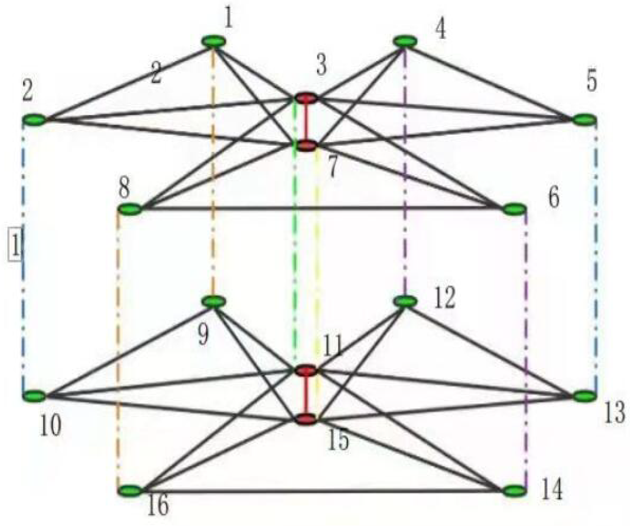
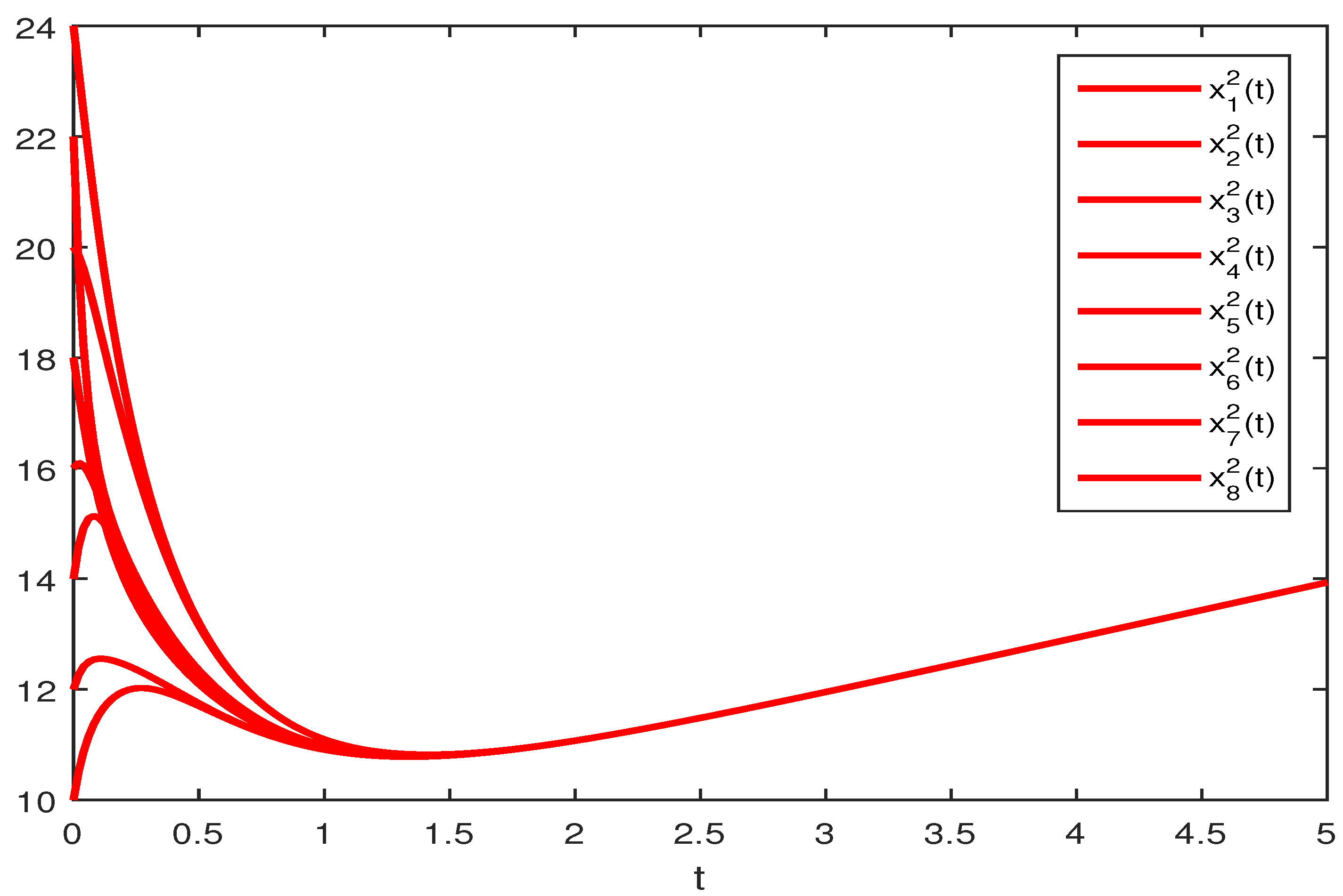
We consider an example of the networked system composed by two-layers (see Figure 3). $M=2$ is the number of layers, the number of nodes within each layer is described as $N=8$, and the dynamics of each node are described as follows:

$$\frac{d{x}_i^k}{dt}=tanh\left(x_i^k\right)+\sum _{j\in N_i}{a}_{ij}(x_j^k-x_i^k)+\sum _{j\in N_i}{b}_{ij}(x_j^{3-k}-x_i^k)$$

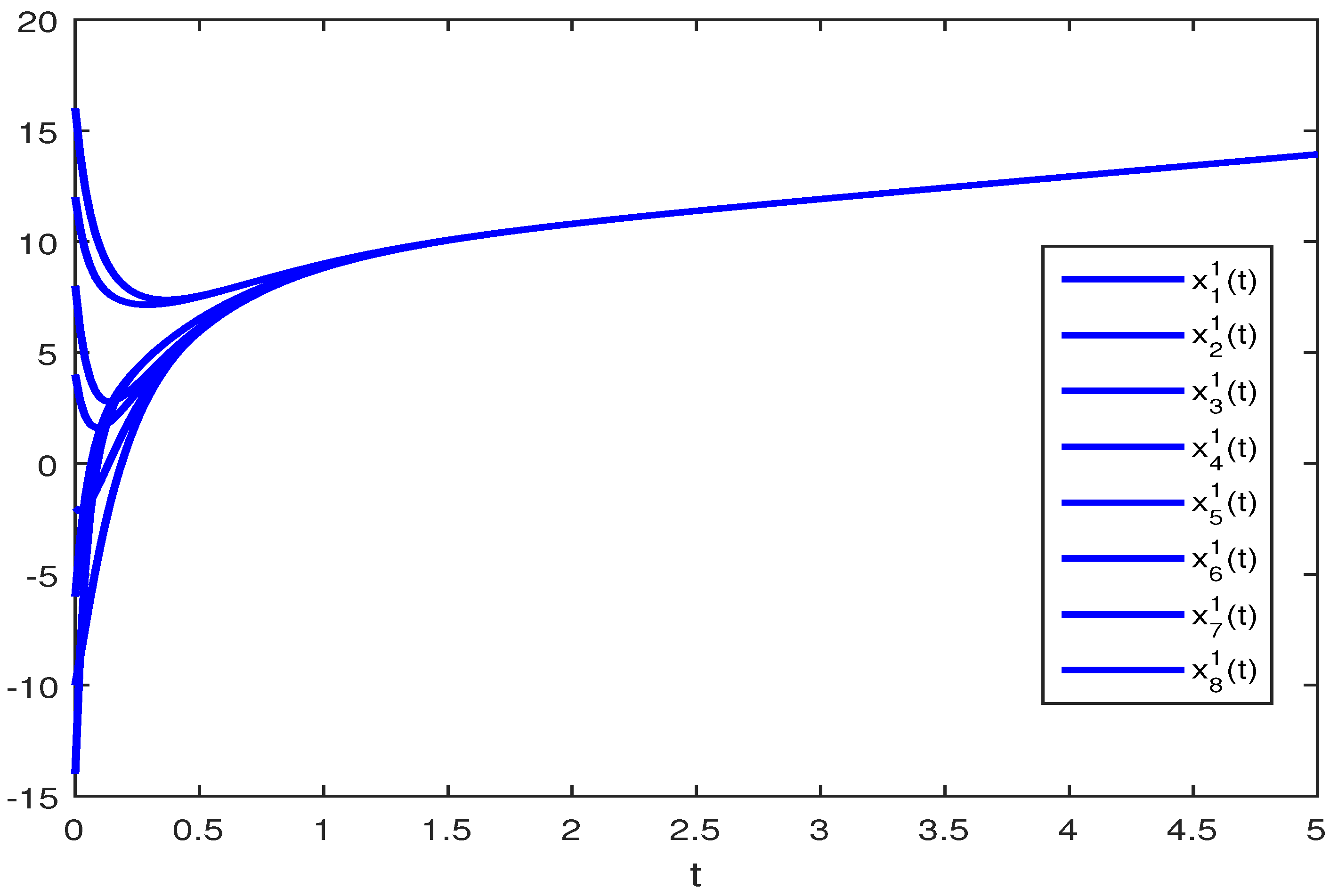
where $x_i^k$ is the state of a node, $tanh\left(x_i^k\right)$ denotes the inherent nonlinear dynamics of the node, $i=1,2,\cdots ,8$, $k=1,2$; $a_{ij}$ represents intra-layer connection, and the connection weight is 2; $b_{ij}$ denotes inter-layer connection, and the connection weight is 1. The initial value of the system is randomly selected, $X_0=[-2,4,-6,8,-10,12,-14,16,10,12,14,16,18,20,22,24]$. Through the simulation, the state trajectory of the system is shown in Figure 4 and Figure 5. It can be seen that the state trajectory of nodes achieves synchronization under the coupling effect. Other situations in this article can also be synchronized in a similar way.

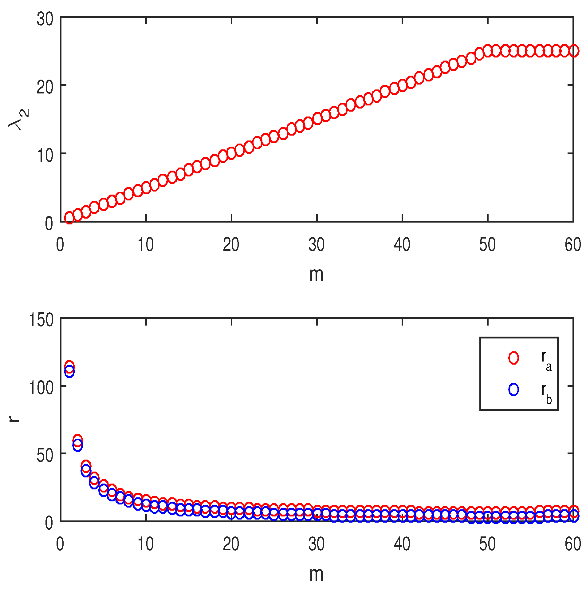
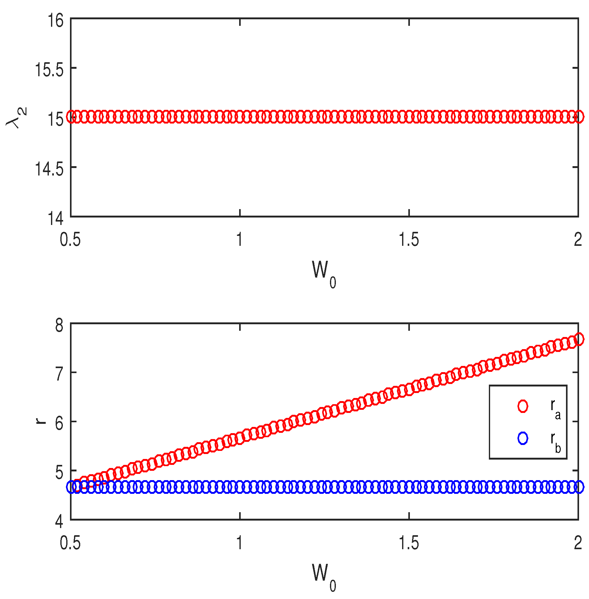
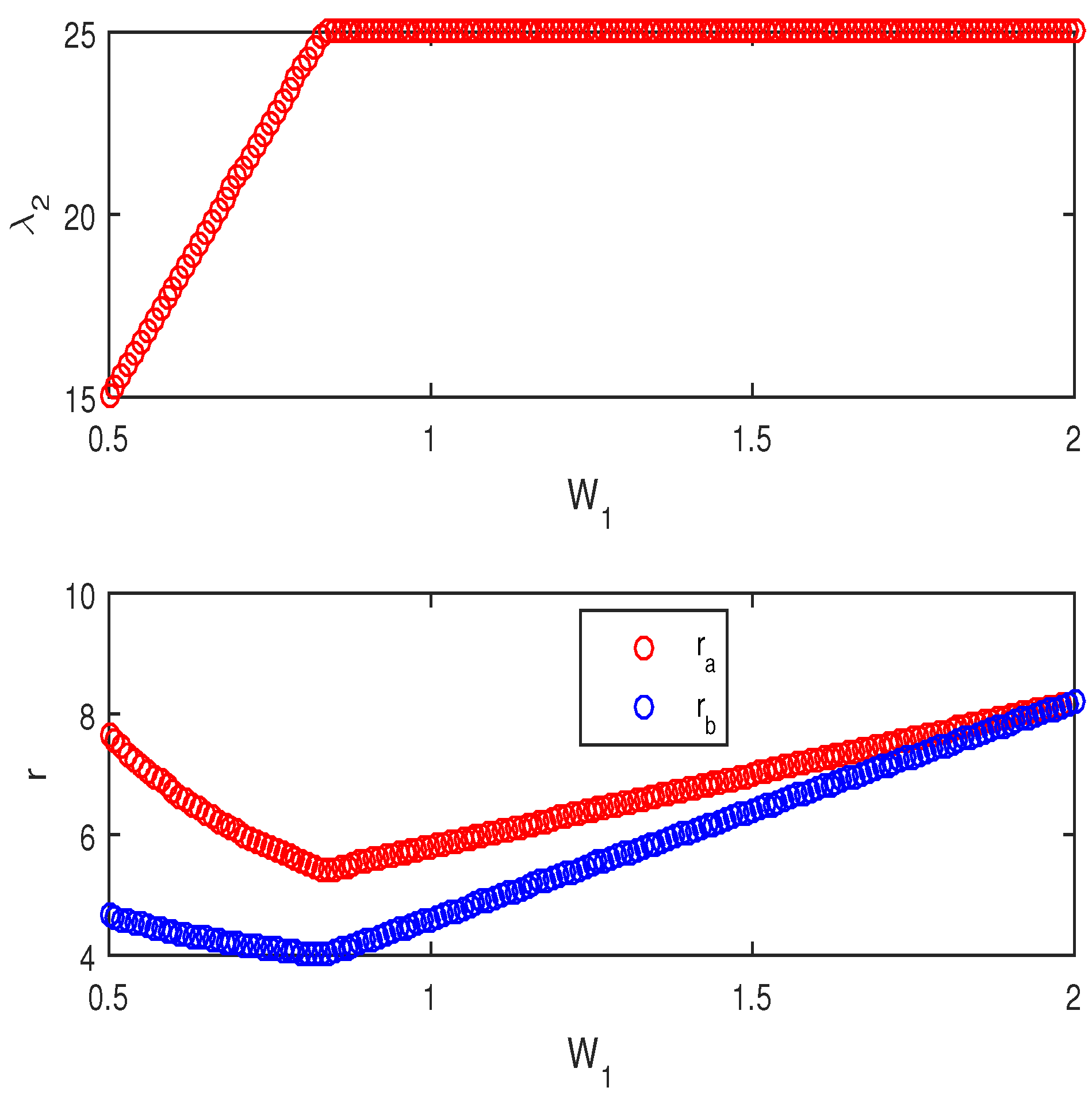
In the following analysis, ${\lambda }_{2a}$ denotes the minimum non-zero eigenvalue of $G_1^K(m,n,k)$ networks, $r_a$ represents the synchronizability of $G_1^K(m,n,k)$ networks when the synchronization domain is bounded; ${\lambda }_{2b}$ represents the minimum non-zero eigenvalue of $G_2^K(m,n,k)$ networks, and $r_b$ represents the synchronizability of $G_2^K(m,n,k)$ networks when the synchronization domain is bounded. From the former section, we have ${\lambda }_{2a}={\lambda }_{2b}$, set ${\lambda }_{2a}={\lambda }_{2b}={\lambda }_2$.

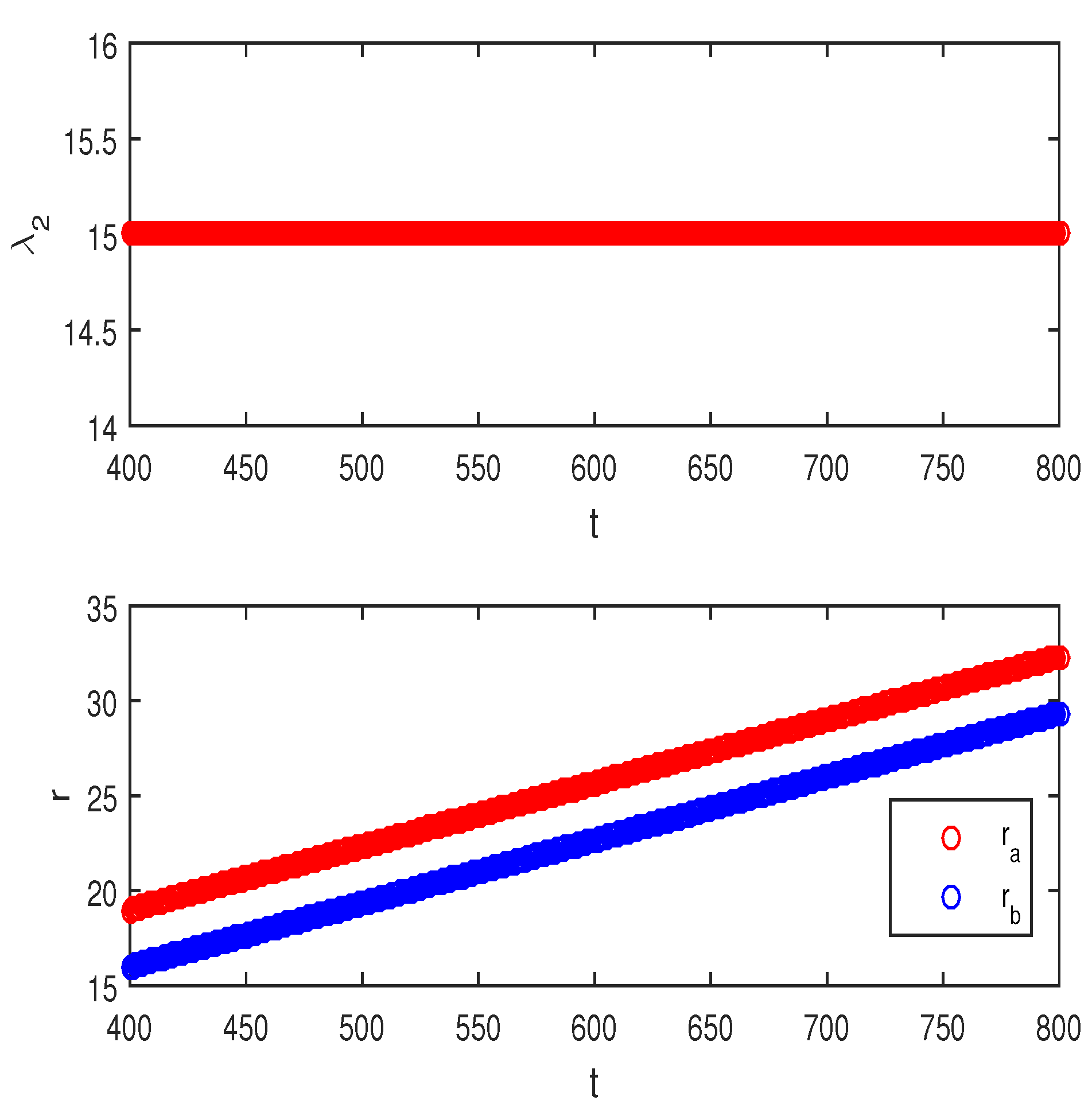
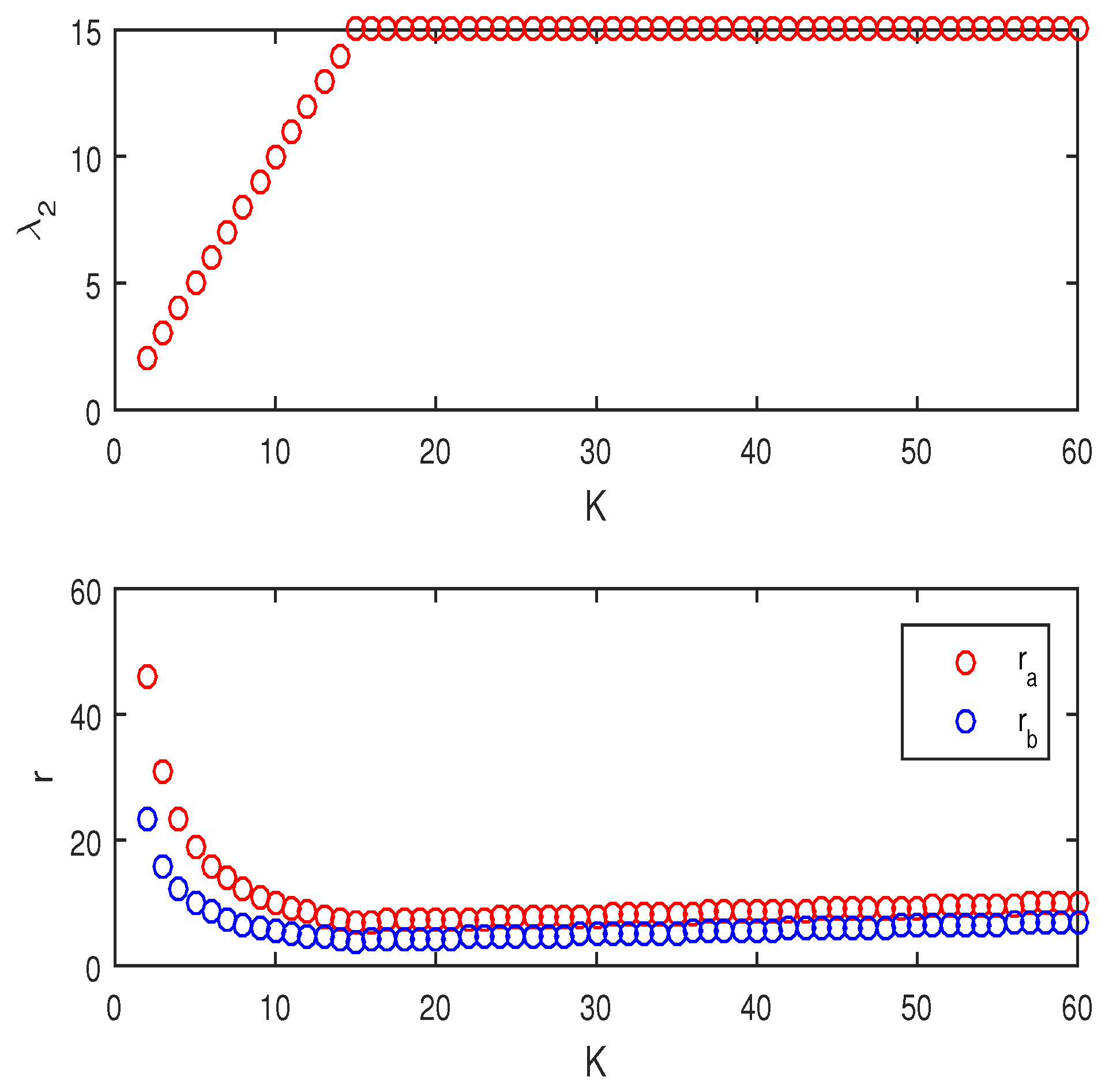
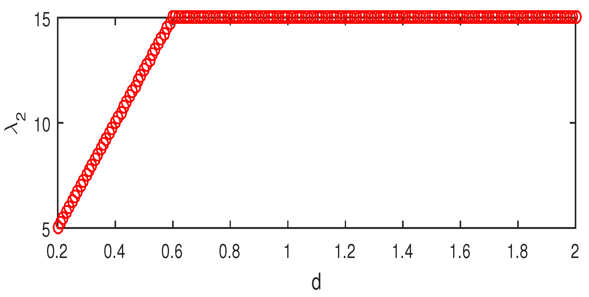
• When the synchronization domain is unbounded, with the increase of $m(m>1)$ in Figure 6, ${\lambda }_2$ monotonically increases from 0 to 25, and then remains unchanged at 25; with the increase of ${\omega }_0$ in Figure 7, ${\lambda }_2$ remains unchanged at 15; with the increase of ${\omega }_1$ in Figure 8, ${\lambda }_2$ monotonically increases from 15 to 25, and then remains unchanged at 25; with the increase of $nk$ in Figure 9, ${\lambda }_2$ remains unchanged at 15; with the increase of K in Figure 10, ${\lambda }_2$ monotonically increases from 2 to 15 and then remains unchanged at 15; with the increase of d in Figure 11, ${\lambda }_2$ monotonically increases from 5 to 15 and then remains unchanged at 15.
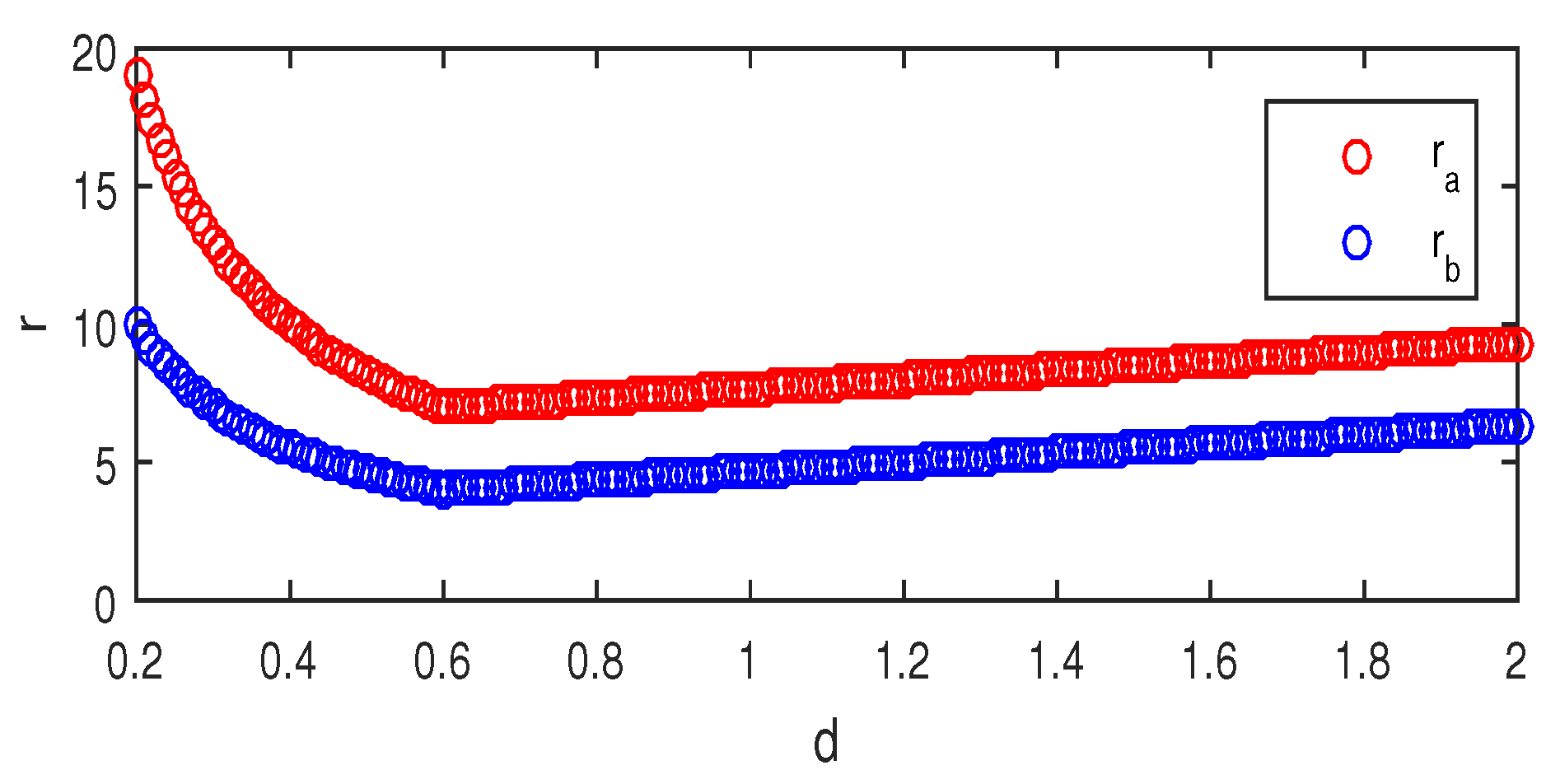
• When the synchronization domain is bounded, with the increase of $m(m>1)$ in Figure 6, $r_a$ decreased rapidly from 114 to 6.2, and then increased slowly to 7, and $r_b$ decreased rapidly from 111 to 3.2, and then increased slowly to 3.4; with the increase of ${\omega }_0$ in Figure 7, $r_a$ increased slowly from 4.6667 to 7.6667, and $r_b$ remains unchanged at 4.6667; with the increase of ${\omega }_1$ in Figure 8, $r_a$ decreased slowly from 7.6667 to 5.4137, and then increased slowly to 8.2, and $r_b$ decreased slowly from 4.6667 to 4.004, and then increased slowly to 8.2; with the increase of $nk$ in Figure 9, $r_a$ increased rapidly from 19 to 32.3333, and $r_b$ increased rapidly from 16 to 29.3333; with the increase of K in Figure 10, $r_a$ decreased rapidly from 46 to 7 and then increased slowly to 10, and $r_b$ decreased rapidly from 23.5 to 4 and then increased slowly to 7; with the increase of d in Figure 11, $r_a$ decreased rapidly from 19 to 7 and then increased slowly to 9.3333, and $r_b$ decreased rapidly from 10 to 4 and then increased slowly to 6.3333.

6. Main Results

6.1. Synchronizability Comparison of the Layered Windmill-Type Networks

When the synchronization domain is unbounded, we found the synchronizability of the $G_1^K(m,n,k)$ and $G_2^K(m,n,k)$ are the same. They are only related to the number of leaders, the coupling strength between the leader nodes and the follower nodes, the number of layers, and the inter-layer coupling strength. The detailed variation relationships are given in

Table 1. Relationships between the parameters affecting $G_1^k(m,n,k)$ networks synchronizability.

		$\mathit{m}\uparrow$	${\mathit{\omega }}_0\uparrow$	${\mathit{\omega }}_1\uparrow$	$\mathit{nk}\uparrow$	$\mathit{K}\uparrow$	$\mathit{d}\uparrow$
${\lambda }_2=min\{Kd,m{\omega }_1\}$	$m{\omega }_1<Kd$	↑	−	↑	−	−	−
	$m{\omega }_1>Kd$	−	−	−	−	↑	↑
$r=(m{\omega }_0+nk{\omega }_1+Kd)/{\lambda }_2$	$m{\omega }_1<Kd$	↓	↑	↓	↑	↑	↑
	$m{\omega }_1>Kd$	↑	↑	↑	↑	↓	↓

↑ strengthen, ↓ weaken, − unchange.

and

Table 2. Relationships between the parameters affecting $G_2^k(m,n,k)$ networks synchronizability.

		$\mathit{m}\uparrow$	${\mathit{\omega }}_0\uparrow$	${\mathit{\omega }}_1\uparrow$	$\mathit{nk}\uparrow$	$\mathit{K}\uparrow$	$\mathit{d}\uparrow$
${\lambda }_2=min\{Kd,m{\omega }_1\}$	$m{\omega }_1<Kd$	↑	−	↑	−	−	−
	$m{\omega }_1>Kd$	−	−	−	−	↑	↑
$r=\left((m+nk){\omega }_1+Kd\right)/{\lambda }_2$	$m{\omega }_1<Kd$	↓	−	↓	↑	↑	↑
	$m{\omega }_1>Kd$	↑	−	↑	↑	↓	↓

↑ strengthen, ↓ weaken, − unchange.

. When the synchronization domain is bounded, the synchronizability of $G_1^K(m,n,k)$ and $G_2^K(m,n,k)$ are related to the inter-layer coupling strength, the number of follower nodes, the coupling strength between the leader nodes and the follower nodes, the number of layers, leader nodes and departments. However, the network $G_1^K(m,n,k)$ is also affected by ${\omega }_0$, the detailed variation relationships are given in Table 1 and Table 2. Whether the synchronization domain is bounded or unbounded, we found the synchronizability of $G_1^K(m,n,k)$ is not stronger than that of the network $G_2^K(m,n,k)$. With the change of the number of leader nodes m, the synchronizability changes rapidly, which shows that the number of leader nodes m plays a major role in the network synchronizability; when there are connections among the leader nodes, the synchronizability of the network may be weakened; the coupling strength among the follower nodes does not affect the synchronizability of the network. These findings can provide a theoretical basis for engineers to design optimization schemes.

6.2. Synchronizability Optimization of the Single-Layer Windmill-Type Network

When the synchronization domain is unbounded, the synchronizability of the network is determined by ${\lambda }_2$; when the synchronization domain is bounded, the synchronizability of the networks model is determined by r. A natural question arises: when do the networks become optimal in the case of bounded and unbounded synchronization domain? The following gives the optimal conditions of variable coupling windmill-type networks, when the synchronization domain is unbounded and bounded.

Theorem 1.

Under the assumption that $nk\ge m$ for the graph structures $G_1(m,n,k)$ and $G_2(m,n,k)$, ${\lambda }_2$ and r are optimal at the same condition, which means $nk=m$, ${\omega }_0={\omega }_1$, $n{\omega }_1={\omega }_2$.

Proof. 

Under the assumption of $nk\ge m$, the minimum nonzero eigenvalue and the maximum eigenvalue of $G_1(m,n,k)$ graphs are discussed, ${\lambda }_2=m{\omega }_1$, ${\lambda }_{max}=max\{m{\omega }_0+nk{\omega }_1,m{\omega }_1+nk{\omega }_1,m{\omega }_1+k{\omega }_2\}$, $r={\lambda }_{max}/{\lambda }_2=max\{{\omega }_0/{\omega }_1+nk/m,1+nk/m,1+k{\omega }_2/m{\omega }_1\}$. □

We discuss the optimization problem in two cases:

• $nk{\omega }_1\ge k{\omega }_2$, thus, $r=max\{{\omega }_0/{\omega }_1+nk/m,1+nk/m\}$, if ${\omega }_0\ge {\omega }_1$, then $r={\omega }_0/{\omega }_1+nk/m\ge 1+nk/m\ge 1+1=2$; if ${\omega }_0\le {\omega }_1$, then $r=1+nk/m\ge 1+1=2$. $r=2$ is the optimal solution in the case of $nk=m$, ${\omega }_0\le {\omega }_1$, $n{\omega }_1\ge {\omega }_2$.
• $nk{\omega }_1\le k{\omega }_2$, thus, $r=max\{{\omega }_0/{\omega }_1+nk/m,1+k{\omega }_2/m{\omega }_1\}$, if ${\omega }_0/{\omega }_1-1\le (k/m)$$({\omega }_2/{\omega }_1-n)$, then $r=1+k{\omega }_2/m{\omega }_1\ge 1+nk{\omega }_1/m{\omega }_1\ge 1+nk/m\ge 1+1=2$, $r=2$ is the optimal solution in the case of $nk=m$, ${\omega }_0\le {\omega }_1$,$n{\omega }_1={\omega }_2$. If ${\omega }_0/{\omega }_1-1\ge (k/m)({\omega }_2/{\omega }_1-n)$, then $r={\omega }_0/{\omega }_1+nk/m\ge {\omega }_0/{\omega }_1+1$, thus $r\ge {\omega }_0/{\omega }_1+1\ge 2$, $r=2$ is the optimal solution in the case of $nk=m$, ${\omega }_0={\omega }_1$, $n{\omega }_1={\omega }_2$.

In contrast for ${\lambda }_2=m{\omega }_1$, the optimal solution can only be obtained in the case of $n{\omega }_1\le {\omega }_2$ and ${\omega }_0\ge {\omega }_1$ and increasing the number of central nodes to $nk$ from m. Then, ${\lambda }_2$ and r are optimal at the same time in the case of $nk=m$, ${\omega }_0={\omega }_1$, $n{\omega }_1={\omega }_2$.

Under the assumption of $nk\ge m$, the minimum nonzero eigenvalue and the maximum eigenvalue of $G_2(m,n,k)$ graphs are discussed, ${\lambda }_2=m{\omega }_1$, ${\lambda }_{max}=max\{m{\omega }_1+nk{\omega }_1,m{\omega }_1+k{\omega }_2\}$, $r={\lambda }_{max}/{\lambda }_2=max\{1+nk/m,1+k{\omega }_2/m{\omega }_1\}$. If $nk{\omega }_1\ge k{\omega }_2$, then $r=1+nk/m\ge 1+1=2$; if $nk{\omega }_1\le k{\omega }_2$, then $r=1+k{\omega }_2/m{\omega }_1\ge 1+nk{\omega }_1/m{\omega }_1\ge 1+nk/m\ge 1+1=2$, $r=2$ is the optimal solution in the case of $nk=m$, $n{\omega }_1\ge {\omega }_2$. Unlike with ${\lambda }_2=m{\omega }_1$, when taking $n{\omega }_1\ge {\omega }_2$, the optimal solution is not obtained. The optimal solution can only be obtained when $n{\omega }_1\le {\omega }_2$ and increasing the number of central nodes to $nk$ from m. Then, ${\lambda }_2$ and r are optimal at the same time in the case of $nk=m$, $n{\omega }_1={\omega }_2$.

There still exist many unsolved problems on variable coupling windmill-type networks, for instance, how to optimize the synchronizability of multi-layer variable coupling windmill-type networks in this paper; for multi-layer variable coupling windmill-type networks, it would be interesting to conduct the further research on how the synchronizability of the windmill-type networks changes when the inter-layer coupling strengths are different.

References

- Tang, L.; Wu, X.; Lu, J.L.J.; D’Souza, R.M. Master stability functions for complete, intralayer, and interlayer synchronization in multiplex networks of coupled Rössler oscillators. Phys. Rev. E 2019, 99, 012304. [Google Scholar] [CrossRef] [Green Version]
- Deng, Y.; Jia, Z.; Deng, G.; Zhang, Q. Eigenvalue spectrum and synchronizability of multiplex chain networks. Phys. A 2020, 537, 122631. [Google Scholar] [CrossRef]
- Xu, M.; Zhou, J.; Lu, J.; Wu, X. Synchronizability of two-layer networks. Eur. Phys. J. B 2015, 88, 240. [Google Scholar] [CrossRef]
- Shen, J.; Tang, L. Intra-layer synchronization in duplex networks. Chin. Phys. B 2018, 27, 100701. [Google Scholar] [CrossRef]
- Wei, X.; Emenheiser, J.; Wu, X.; Lu, J.; D’Souza, R.M. Maximizing synchronizability of duplex networks. Chaos 2018, 28, 013110. [Google Scholar] [CrossRef] [Green Version]
- Aguirre, J.; Sevilla, R.E.; Gutirrez, R.; Papo, D. Synchronization of interconnected networks: The role of connector nodes. Phys. Rev. Lett. 2014, 112, 248701. [Google Scholar] [CrossRef] [PubMed] [Green Version]
- Deng, Y.; Jia, Z.; Yang, F. Synchronizability of multi-layer star and star-ring Networks. Discret. Dyn. Nat. Soc. 2020, 2020, 9143917. [Google Scholar] [CrossRef]
- Wei, J.; Wu, X.; Lu, J.; Wei, X. Synchronizability of duplex regular networks. Europhys. Lett. 2017, 120, 20005. [Google Scholar] [CrossRef]
- Hu, C.; He, H.; Jiang, H. Synchronization of complex-valued dynamic networks with intermittently adaptive coupling: A direct error method. Automatica 2019, 112, 108675. [Google Scholar] [CrossRef]
- Chutani, M.; Tadic, B.; Gupte, N. Hysteresis and synchronization processes of Kuramoto oscillators on high-dimensional simplicial complexes with the competing simplex-encoded couplings. Phys. Rev. E 2021, 104, 034206. [Google Scholar] [CrossRef] [PubMed]
- Huang, D.; Jiang, H.; Yu, Z.; Hu, C.; Fan, X. Cluster-delay consensus in MASs with layered intermittent communication: A multi-tracking approach. Nonlinear Dyn. 2019, 95, 1713–1730. [Google Scholar] [CrossRef]
- Hu, C.; He, H.; Jiang, H. Fixed/preassigned-time synchronization of complex networks via improving fixed-time stability. IEEE Trans. Cybern. 2019, 99, 1–11. [Google Scholar] [CrossRef] [PubMed]
- Yan, H.; Zhou, J.; Li, W.; Lu, J.; Fan, R. Superdiffusion criteria on duplex networks’. Chaos 2021, 31, 073108. [Google Scholar] [CrossRef]
- Cencetti, G.; Battiston, F. Diffusive behavior of multiplex networks. New J. Phys. 2019, 21, 035006. [Google Scholar] [CrossRef]
- Tejedor, A.; Longjas, A.; Foufoula-Georgiou, E.; Georgiou, T.T.; Moreno, Y. Diffusion dynamics and optimal coupling in multiplex networks with directed Layers. Phys. Rev. X 2018, 8, 031071. [Google Scholar] [CrossRef] [Green Version]
- Wang, X.; Tejedor, A.; Wang, Y.; Moreno, Y. Unique superdiffusion induced by directionality in multiplex networks. New J. Phys. 2021, 23, 013016. [Google Scholar] [CrossRef]
- Hong, M.; Sun, W.; Liu, S.; Xuan, T. Coherence analysis and Laplacianenergy of recursive trees with controlled initial states. Front. Inf. Technol. Electron. Eng. 2020, 21, 931–938. [Google Scholar] [CrossRef]
- Dankulov, M.; Tadi, B.; Melnik, R. Spectral properties of hyperbolic nanonetworks with tunable aggregation of simplexes. Phys. Rev. E 2019, 100, 012309. [Google Scholar] [CrossRef] [Green Version]
- Huang, D.; Zhu, J.; Yu, Z.; Jiang, H. On consensus index of triplex star-like networks: A graph spectra approach. Symmetry 2021, 13, 1248. [Google Scholar] [CrossRef]
- Li, Y.; Zhong, J.; Lu, J.; Wang, Z.; Alssadi, F. On Robust Synchronization of Drive-Response Boolean Control networks with Disturbances. Math. Probl. Eng. 2018, 2018, 1737685. [Google Scholar] [CrossRef] [Green Version]
- Li, J.; Luan, Y.; Wu, X.; Lu, J. Synchronizability of double-layer dumbbell net-works’. Chaos 2021, 31, 073101. [Google Scholar] [CrossRef] [PubMed]
- Zhang, L.; Wu, Y. Synchronizability of Multilayer networks With K-nearest-neighbor Topologies. Front. Phys. 2020, 8, 571507. [Google Scholar] [CrossRef]
- Wang, L.; Jia, X.; Pan, X.; Xia, C. Extension of synchronizability analysis based on vital factors: Extending validity to multilayer fully coupled networks. Chaos Solitons Fractals 2020, 142, 110484. [Google Scholar] [CrossRef]
- Duan, Z.; Chen, G.; Huang, L. Disconnected synchronized regions of complex dynamical networks. IEEE Trans. Autom. Control. 2009, 54, 845–849. [Google Scholar] [CrossRef] [Green Version]
- Kooij, R. On generalized windmill graphs. Linear Algebra Its Appl. 2019, 565, 25–46. [Google Scholar] [CrossRef]
- Sun, W.; Li, Y.; Liu, S. Noisy consensus dynamics in windmill-type graphs. Chaos 2020, 30, 123131. [Google Scholar] [CrossRef]
- Granell, C.; Gomez, S.; Arenas, A. Dynamical Interplay between Awareness and Epidemic Spreading in Multiplex Networks. Phys. Rev. Lett. 2013, 111, 128701. [Google Scholar] [CrossRef] [Green Version]
- Rakshit, S.; Majhi, S.; Bera, B.K.; Sinha, S.; Ghosh, D. Time-varying multiplex network: Intralayer and interlayer synchronization. Phys. Rev. E 2017, 96, 062308. [Google Scholar] [CrossRef]
Figure 1.
Examples of single-layer windmill-type graphs.
Figure 2.
Examples of double-layer windmill-type graphs.
Figure 3.
An example of double-layer windmill-type graphs.
Figure 4.
State trajectories of the first layer.
Figure 5.
State trajectories of the second layer.
Figure 6.
and r change with m. .
Figure 7.
and r change with . .
Figure 8.
Figure 9.
and r change with t, . .
Figure 10.
and r change with K. .
Figure 11.
and r change with d. .