Mathematical Modeling and Optimal Control of the Hand Foot Mouth Disease Affected by Regional Residency in Thailand

Abstract

Hand, foot and mouth disease (HFMD) is a virulent disease most commonly found in East and Southeast Asia. Symptoms include ulcers or sores, inside or around the mouth. In this research, we formulate the dynamic model of HFMD by using the SEIQR model. We separated the infection episodes where there is a higher outbreak and a lower outbreak of the disease associated with regional residency, with the higher level of outbreak occurring in the urban region, and a lower outbreak level occurring in the rural region. We developed two different optimal control programs for the types of outbreaks. Optimal Control Policy 1 (OPC1) is limited to the use of treatment only, whereas Optimal Control Policy 2 (OPC2) includes vaccination along with the treatment. The Pontryagin’s maximum principle is used to establish the necessary and optimal conditions for the two policies. Numerical solutions are presented along with numerical sensitivity analyses of the required control efforts needed as the control parameters are changed. Results show that the time $t_{max}$ required for the optimal control effort to stay at the maximum amount $u_{max}$ exhibits an intrinsic logarithmic relationship with respect to the control parameters.

1. Introduction

Hand, foot and mouth Disease (HFMD) is an infectious disease attributable to a viral infection. It is most commonly caused by either coxsackievirus A16 (CV-A16) or enterovirus 71 (EV71). It is most frequently seen in the summer and rainy seasons. HFMD mainly affects children under the age of 10 with most being younger than five years. It can also occur in older children and young adults [1]. HFMD is contracted through close personal contact, for instance, direct contact with the fluids from skin blisters, nose and throat secretions (saliva sputum or nasal mucus) and stools of infected people. The disease also spreads through the respiratory route when the infected person coughs or sneezes, leading to droplets being emitted into the air. Other possible routes include contact with any contaminated objects and surfaces with fluid from the blisters. Thus, it can spread easily in places where children are close together such as schools, kindergartens and childcare centers. Infected people are most contagious during the first week after the infection starts and may continue for several weeks, even after symptoms have disappeared.

The incubation period of HFMD is 3 to 6 days after contact with an infected person. After this period, symptoms may or may not appear. Most adults exhibit no symptoms, but they can still spread the virus to others. The sign of infection may be a mild fever or symptoms with fever such as sore throat, runny nose, cough, tiredness and loss of appetite. The fever usually lasts 1 to 2 days. After the second day, tiny painful blisters develop on the inside of the mouth, including the tongue, gums and cheeks. Small red dots may appear on the fingers, palms of hands, buttocks, soles of feet and side of the toes. These dots may turn into blisters. The spots and blisters usually last longer than a week and one should allow these blisters to dry out naturally. HFMD is a mild illness in which most people completely recover in 7 to 10 days without medical treatment. The fever can be alleviated with antipyretics and pain can be treated with Acetaminophen. Serious signs of HFMD are persistent fever, abnormal movements, rapid breathing, chest pain and fatigue. A few children may have experienced central nervous system damage, which leads to aseptic meningitis, encephalitis and polio-like paralysis [2]. Large outbreaks of HFMD in Asia are associated with EV71 and have been reported since 1997. There are many countries which have been reporting larger numbers of cases in recent years. In the first half of 2018, Malaysia reported 35,886 cases, followed by Vietnam with 22,746 cases and Singapore with 21,595 cases [3]. Thailand reported between 2000 and 18,000 cases, with 2–6 deaths annually between the period of 2007–2011 [4]. The prevalence of HFMD in Thailand during 2012–2016 is usually associated with the CV-A6 or CV-A16 virus [5]. In 2018, the Thai Department of Disease Control reported 67,912 HFMD cases with 6 deaths. The greatest number of cases occurred in children aged 1 year old (26.04%) followed by those aged 2 years old (23.57%) and 3 years old (18.87%). Provinces with the highest incidences were Chanthaburi and Phayao in 2017 [6]. Prachuap Khiri Khan and Surat Thani topped the list in 2019 [7]. There are several factors attributed to the epidemiology of HFMD. Previous reports from cases in China and Korea indicate the importance of hygiene against the HFMD infection; that is, unsanitary practices result in a higher prevalence of the disease [8,9]. Studies comparing the urban against the rural areas agreed that the rural areas conferred higher risks of the disease, particularly in East Asian countries such as Taiwan and China [10,11]. In the Thai context, however, the concept of urban is mainly that the population density is greater, along with high value of socioeconomic status, and greater establishment of health care infrastructures. The concept of rural mainly concerns lower population density, with lower socioeconomic statuses, which also reflects their access to the health care system [12]. As an example,

Table 1. The occurrences of the HFMD in Nakhon Ratchasima and Chaiyaphum between 2017 and 2021 (per 100,000 population) [13].

9	Nakhon Ratchasima	Chaiyaphum
2018	110.70	100.42
2019	99.69	70.04
2020	5.99	5.97
2021	35.16	23.81

compares the HFMD cases between two provinces in the northeastern region of Thailand, namely Nakhon Ratchasima, which is dubbed the main gateway to the northeast and has been heavily urbanized in recent decades, against Chaiyaphum, a neighboring province to Nakhon Ratchasima mostly composed of rural areas, during the period of 2017–2021. As can be seen, the occurrences of the HFMD in Chaiyaphum is somewhat lower than that of Nakhon Ratchasima. Note also that the HFMD cases have been significantly reduced in the last two years, owing to the spread of COVID-19, which prompted the government to issue lockdown measures.

In 2014, Samanta [14] developed a SEI_AI_SQRS model of HFMD with varying total population size. The author also introduced saturation incidence rate and discrete time delay to analyze this model with the effect of pulse vaccination. Li et al. [15] considered the HFMD data of China in 2009 and constructed an epidemic model to fit the data. They obtained the optimal parameter values of the SEIQRS model and verified the rationality of these parameters by applying the chi-squared test. Zhu et al. [16] proposed an SEIQRS model of HFMD with a periodic transmission rate to investigate the spread of seasonal HFMD based on the statistics data for Wenzhou province in China. In 2017, Wu [17] proposed an SEIR model with a standard incidence rate to describe the transmission of HFMD. In particular, an algorithm for estimating the value of the basic reproduction number for both yearly and real time of HFMD transmission was also presented. Chadsuthi and Wichapeng [18] proposed a SEIHRW model to investigate the effect of indirect transmission via free-living viruses in contaminated environments and the impact of asymptomatic individuals in the model. The model can also be fitted to the reported data on hospitalized individuals during the HFMD endemic in Bangkok in 2016. In 2018, Tan and Cao [19] formulated a SEIVT epidemic model with vaccination to study the transmission of HFMD. The optimized control measures for the HFMD model were applied to the HFMD model to minimize the cost of the intervention and the number of infected people. In 2018, Wang et al. [20] considered the daily number of cases of HFMD in Chongqing, China, between 2009 and 2014, and the values of several meteorological parameters for this city during the same period. The parameters that they considered were the daily mean temperatures, the mean relative humidity, the mean pressure, the mean wind speed and the daily duration of the sunlight. They then looked for the statistical correlation between the seasonal variations of the incidence of HFMD and the six meteorological parameters recorded in the city of Chongqing in the period between 2009 and 2014. They found similar lag times other correlations between the seasonal variations of the diseases and the parameters when considering the data for the summer months (from April to September) and the data for the winter months (from October to March). This caused them to consider the evolution of HFMD to be different depending on whether the infections occurred during a higher or a lower episode of the outbreak. Other recent developments have also involved the fractional order systems [21,22,23,24], predator–prey point of views [25,26,27], as well as the use of existing epidemiological modeling to predict peak responses of a pandemic with complex dynamics [28,29]. Multiple patch frameworks have also been proposed to deal with the heterogeneity of the pandemics [30,31,32,33]. Although these frameworks allow for a fuller investigation of the associated heterogeneity effects of a pandemic, the inclusion of a residence matrix in these models means that the resulting epidemic models are significantly more complex with diminished traceability in analysis.

The use of optimal control theories has garnered attention from epidemiological modelers in recent years. Rodrigues [34] used optimal control theory to determine the parameters needed to optimally decrease the number of mosquitoes of the dengue disease over a short time and at minimal cost. Pongsumpun et al. [35] applied optimal control to the dengue system subjected to vertical transmission. Researchers have also applied the optimal control theory to reduce Zika cases [36,37,38] and Chikungunya [39]. These works have concentrated on the use of optimal control on a single policy. Recent work on the use of optimal control in multiple policy has also been studied in ref. [40].

The contribution of this research is to develop a simplified mathematical model of the progression of the HFMD pandemic while taking into account the effect of residency. The need for this comes from the fact that the transmission of HFMD is different in urban and rural areas and in public health policy practices. A lot of the differences are due to the economical wealth of the populace in the two types of area. A good portion of the children in the urban areas attend expensive private schools, whereas the rest of the children go to inexpensive government schools. This is important in that one of the important venues for the transmission of HFMD is schools. The prevention of the spread of HFMD and other communicative diseases in the urban area is the use of medicines and the establishment of hospitals, while in the rural areas, it is the use of quarantines and government health clinics. In the rural provinces, it is quite common to completely shut down the province and set up field hospitals in the local Wats (Buddhist Temples). The model itself should not be too overly complex as to diminish the traceability during mathematical analysis. In fact, a minimal modeling concept similar to the work of ref. [41] is desired, as to minimize the number of unidentifiable parameters in the model. An optimal control is also derived based on the developed model. Numerical analyses are then given to investigate the optimal control efforts needed to achieve the required control, so that the epidemiologist may ascertain beforehand the required efforts of halting the disease progression.

2. Methodology

2.1. Mathematical Model

The mathematical model governing the dynamics of HFMD for urban and rural Thailand was developed using the $S{E}_h{E}_l{I}_h{I}_{l}QR$ model, where the entire human population is separated into susceptible, exposed, infectious, quarantined and recovered. The exposed individuals’ compartment is subdivided into one for the urban region, and one for the rural region. Note that for all intents and purposes of the modeling, we include the asymmetrical infectious individuals into this class, since these individuals can transmit the disease without displaying the symptoms. Likewise, the infected compartment is further subdivided into the urban and rural regions. Previous studies in the literature have indicated that rural and urban areas strongly correlate with the epidemiology of HFMD, particularly in East Asian countries. Note that a common susceptible population group is assumed, since in the Thai context, the Thai Ministry of Public Health takes the macro view of the epidemiology in a province; that is, the Ministry looks at the province as a single entity. The province itself comprises both rural and urban areas. Since most of the occurrences of HFMD are younger than 10, with similar percentages in both areas [6,7], the member of the exposed (which also includes the asymptomatic infected populations) and infected classes come into contact in different ways with respect to their residence. In the rural areas, these members live far enough from one another so that the only possibility of contact will be through government-funded schools. In the urban areas, the possibility of contact can be through private schools and malls. The residents in both areas come together when they gather food in a common local market or a weekly floating market, since it is customary for Thai residents, from both rural and urban areas of a province (especially Nakhon Ratchasima and Chaiyaphum), to shop at a weekly floating market for inexpensive food. Since the number of contacts will be different in rural and urban areas, the rate of transmission, which includes the duration of contact, will also be different. Although the full effect of heterogeneity has been investigated with multiple patch frameworks [30,31,32,33], these frameworks are not consistent with the practice of the Thai Ministry of Health. Moreover, in terms of the mathematical analyses, these frameworks would then require an addition of three additional compartments to the current $S{E}_h{E}_l{I}_h{I}_{l}QR$ model, namely, two susceptible classes, two quarantine classes and two recovered individuals’ classes, as well as the insertion of a residence times matrix between the susceptible classes, the exposed classes and the infected classes. The resultant model would be too overly complicated for analysis, in that even determining the endemic fixed point of such a model can result in a heavy loss of traceability [33].

The main aim of our work is to work with a model which is not too overly complicated but at the same time describes to the situation within Thailand and captures the main dynamics which allow for traceable analysis of spread of HFMD in Thailand. Considering this, the effect of residency is captured in the model simply by using distinct transmission rates ${\beta }_h$ and ${\beta }_l$. The use of a single rate of quarantine $q$ derives from the fact that Thailand has quite a strong health volunteering network in every province. These volunteers are dwellers who are trained in basic health care management and communication with the professional health care facilities and evaluated yearly by the ministry authorities [42]. The use of digital technology has also helped these volunteers in quarantining unwell people from various communicable diseases, including dengue fever, HFMD and, more recently, the COVID-19 pandemic. These volunteers ensure that the rate of detection of infectious individuals remain more or less the same in both rural and urban regions. The model is hereby formulated by the following system of differential equations:

$$\begin{array}{l}{S}^{\prime }=d{N}_T-({\beta }_h+{\beta }_l)S(I_h+I_l)-dS\\ {E_h}^{\prime }={\beta }_{h}S(I_h+I_l)-\left(\theta +d\right)E_h\\ {E_l}^{\prime }={\beta }_{l}S(I_h+I_l)-\left(\theta +d\right)E_l\\ {I^{\prime }}_h=\theta E_h-(d+q)I_h\\ {I^{\prime }}_l=\theta E_l-(d+q)I_l\\ Q^{\prime }=q\left(I_h+I_l\right)-\left(r+d\right)Q\\ R^{\prime }=rQ-dR\end{array}$$

(1)

where $S$ is the number of susceptible humans at time t; $E_h$ is the number of exposed human individuals at time $t$ for the higher outbreak (urban) region; $E_l$ is the number of exposed human individuals at time $t$ for the lower outbreak (rural) region; $I_h$ is the number of infectious human individuals at time t for the higher outbreak (urban) region; $I_l$ is the infectious human individuals at time t for the lower outbreak (rural) region; $Q$ denotes the quarantine human population at time t; $R$ denotes the recovered human population at time t; $N_T$ is the total number of human population; ${\beta }_h$ is the transmission rate of the hand foot mouth disease for the rural region; ${\beta }_l$ is the transmission rate of the hand foot mouth disease for the urban region; $d$ is the death rate; $IIP$ is the intrinsic incubation period of the hand foot mouth disease, with $\theta =\frac{1}{IIP}$ for clarity;$q$ is the quarantine rate, and$r$ is the recovery rate.

This model can be normalized by defining the following:

$$\begin{array}{l}{S}_N=\frac{S}{N_T},\hspace{0.17em}\hspace{0.17em}\hspace{0.17em}\hspace{0.17em}{E}_{hN}=\frac{E_h}{N_T},\hspace{0.17em}\hspace{0.17em}\hspace{0.17em}\hspace{0.17em}{E}_{lN}=\frac{E_l}{N_T},\\ I_{hN}=\frac{I_h}{N_T},\hspace{0.17em}\hspace{0.17em}\hspace{0.17em}\hspace{0.17em}{I}_{lN}=\frac{I_l}{N_T},\hspace{0.17em}\hspace{0.17em}\hspace{0.17em}\hspace{0.17em}{Q}_N=\frac{Q}{N_T},\hspace{0.17em}\hspace{0.17em}\hspace{0.17em}\hspace{0.17em}{R}_N=\frac{R}{N_T}\end{array}$$

The normalized model can now be written:

$$\begin{array}{l}{S_N}^{\prime }=d-({\beta }_h+{\beta }_l)S_N(I_{hN}+I_{lN})-d{S}_N\\ {E_{hN}}^{\prime }={\beta }_h{S}_N(I_{hN}+I_{lN})-\left(\theta +d\right)E_{hN}\\ {E_{lN}}^{\prime }={\beta }_l{S}_N(I_{hN}+I_{lN})-\left(\theta +d\right)E_{lN}\\ {I^{\prime }}_{hN}=\theta E_{hN}-(d+q)I_{hN}\\ {I^{\prime }}_{lN}=\theta E_{lN}-(d+q)I_{lN}\\ {Q_N}^{\prime }=q\left(I_{hN}+I_{lN}\right)-\left(r+d\right)Q_N\\ {R_N}^{\prime }=r{Q}_N-d{R}_N\end{array}$$

(2)

Note that there are no exogenous deaths resulting from the infection rates defined above. The entire population is taken to be that of the province which includes the urban as well as the rural regions in accordance with the Thai Ministry of Public Health. It is thus assumed to be constant for all times, $t$, so that the following holds:

$$S+E_h+E_l+I_h+I_l+Q+R=N_T$$

2.2. Stability Analysis

The equilibrium points or fixed points of Equation (1) are found by setting the right-hand side of all subequations comprising Equation (1) to zero and solved for the respective variables. The computed equilibrium points are:

$$\begin{array}{l}{E}_0=\left(N_T,0,0,0,0,0,0\right)\\ E_1=\left(S^{*},E_h^{*},E_l^{*},I_h^{*},I_l^{*},Q^{*},R^{*}\right)\end{array}$$

(3)

where:

$$\begin{array}{l}{S}^{*}=\frac{(\theta +d)(d+q)}{\theta ({\beta }_h+{\beta }_l)}\\ E_h^{*}=\frac{{\beta }_{h}d\left[({\beta }_h+{\beta }_l)N_T-q-d(1+(1/\theta )(d+q))\right]}{(\theta +d){({\beta }_h+{\beta }_l)}^2}\\ E_l^{*}=\frac{{\beta }_{l}d\left[({\beta }_h+{\beta }_l)N_T-q-d(1+(1/\theta )(d+q))\right]}{(\theta +d){({\beta }_h+{\beta }_l)}^2}\\ I_h^{*}=\frac{{\beta }_{h}d\left(-1+\frac{\theta ({\beta }_h+{\beta }_l)N_T}{(\theta +d)(d+q)}\right)}{{({\beta }_h+{\beta }_l)}^2}\\ I_l^{*}=\frac{{\beta }_{l}d\left(-1+\frac{\theta ({\beta }_h+{\beta }_l)N_T}{(\theta +d)(d+q)}\right)}{{({\beta }_h+{\beta }_l)}^2}\\ Q^{*}=\frac{-dq\theta (-({\beta }_h+{\beta }_l)N_T+q+d(1+(1/\theta )(d+q))}{({\beta }_h+{\beta }_l)(\theta +d)(d+q)(d+r)}\\ R^{*}=\frac{-q\theta (-({\beta }_h+{\beta }_l)N_T+q+d(1+(1/\theta )(d+q))r}{({\beta }_h+{\beta }_l)(\theta +d)(d+q)(d+r)}\end{array}$$

The value of $R_N$, which is the basic reproduction number of the unnormalized model of Equation (1), can be noted from the expressions of $I_h^{*}$ and $I_l^{*}$ as:

$$R_N=\frac{\theta ({\beta }_h+{\beta }_l)N_T}{(d+\theta )(d+q)}$$

The basic reproduction number $R_0$ requires the use of the normalized model given by Equation (2), which will be simply the ratio of $R_N/N_T$ and thus given by:

$$R_0=\frac{\theta ({\beta }_h+{\beta }_l)}{(d+\theta )(d+q)}$$

To ease the algebraic complexities in the steps of stability analysis, the computed endemic equilibrium points can be rewritten in terms of the number $R_N$:

$$\begin{array}{l}{S}^{*}=\frac{N_T}{R_N}\\ E_h^{*}=\frac{{\beta }_{h}d(d+q)(R_N-1)}{({\beta }_h^2+{\beta }_l^2)\theta }\\ E_l^{*}=\frac{{\beta }_{l}d(d+q)(R_N-1)}{({\beta }_h^2+{\beta }_l^2)\theta }\\ I_h^{*}=\frac{{\beta }_{h}d(R_N-1)}{({\beta }_h^2+{\beta }_l^2)}\\ I_l^{*}=\frac{{\beta }_{l}d(R_N-1)}{({\beta }_h^2+{\beta }_l^2)}\\ Q^{*}=\frac{dq(R_N-1)}{(d+r)({\beta }_h+{\beta }_l)}\\ R=\frac{qr(R_N-1)}{(d+r)({\beta }_h+{\beta }_l)}\end{array}$$

(4)

The stability analysis of the system will be carried out using the eigenvalues approach, even though this is a complex system involving more than three variables. This approach has previously been carried out in various other works in the modeling of other epidemics with similar levels of complexity. Some recent examples include the works in [43,44,45].

Proposition 1.

The equilibrium state E₀ is asymptotically stable when$R_0$is less than one.

Proof of Proposition 1.

The proof of Proposition 1 is given in Appendix A.1. □

Proposition 2.

The equilibrium state E₁ is asymptotically stable when$R_0$is above unity.

Proof of Proposition 1.

The proof of Proposition 1 is given in Appendix A.2. □

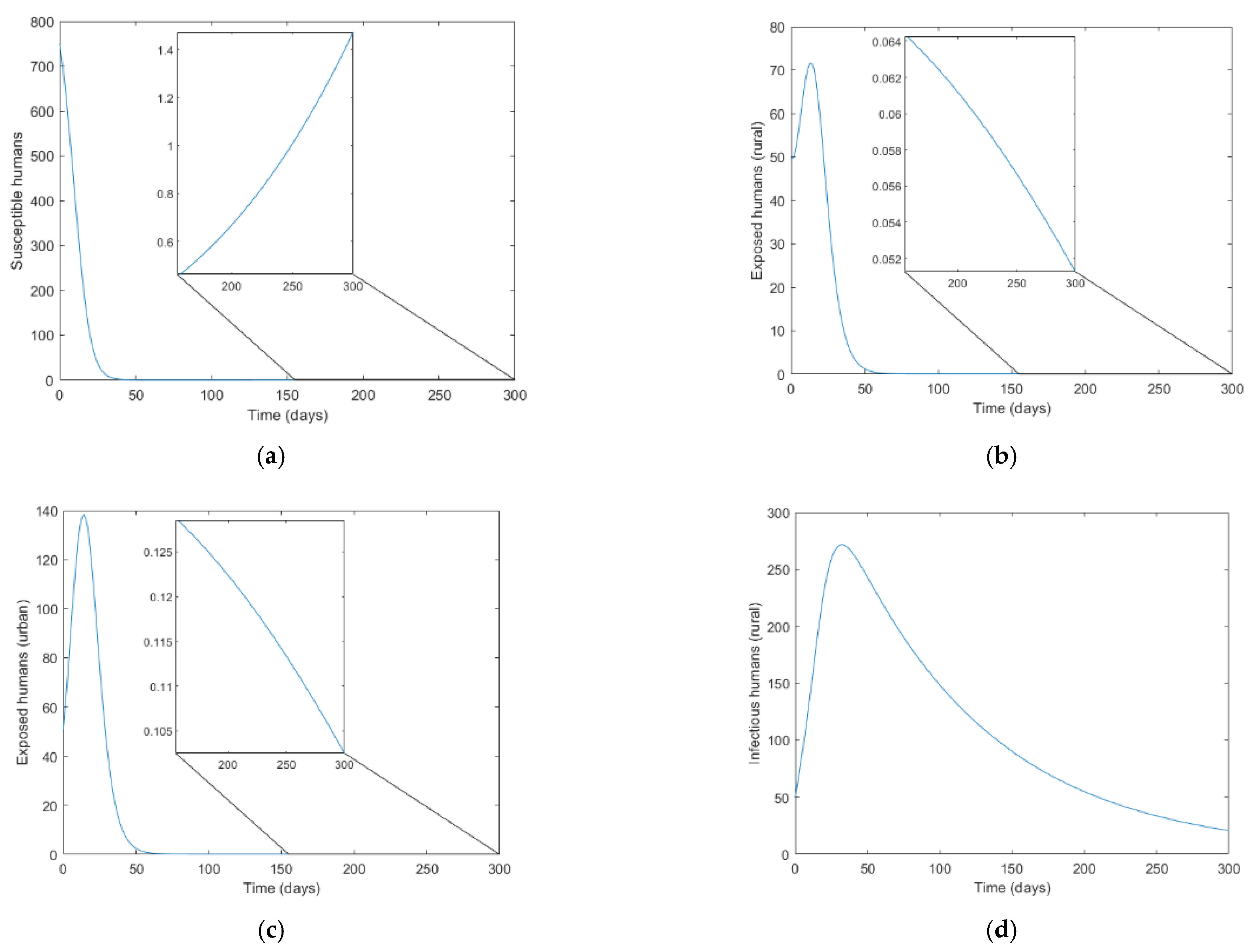
2.3. Numerical Simulation

To demonstrate the stability of the endemic equilibrium, we numerically simulate the trajectories of the solutions of the model described by Equation (1) for $N_T=1000$. We note that the value of the basic reproduction number is $R_0$ = 8.9883. The numerical values of the parameters used are:

The initial conditions for the simulation are:

$$\begin{array}{ll}{y}_0& =[S(0),E_h(0),E_l(0),I_h(0),I_l(0),Q(0),R(0)]\\ & =[750,50,50,50,50,50,0]\end{array}$$

The simulation was conducted with the use of a differential equation solver in Matlab. Figure 1 shows the simulated numerical results for the system of Equation (1) with the parameters listed in

Table 2. The epidemiological parameters used in Equation (1).

Epidemiological Parameter	Value	Comments
${\beta }_h$	0.0002	Unknown, investigated
${\beta }_l$	0.0001	Unknown, investigated
d	$1/(76\times 365)$	Expected life expectancy of Thailand [46]
$\theta$	1/6	ref. [47]
$q$	1/30	ref. [3]
r	1/50	ref. [3]

and with the above initial conditions. Note that the endemic equilibrium points as calculated from Equation (4) are:

$$\begin{array}{l}{S}^{*}=11.1255,\hspace{0.17em}\hspace{0.17em}\hspace{0.17em}\hspace{0.17em}{E}_h{}^{*}=0.2566,\hspace{0.17em}\hspace{0.17em}\hspace{0.17em}\hspace{0.17em}{E}_l^{*}=0.1604,\\ I_h^{*}=1.2817,\hspace{0.17em}\hspace{0.17em}\hspace{0.17em}\hspace{0.17em}{I}_l^{*}=0.6408,\hspace{0.17em}\hspace{0.17em}\hspace{0.17em}\hspace{0.17em}{Q}^{*}=0.7115,\hspace{0.17em}\hspace{0.17em}\hspace{0.17em}\hspace{0.17em}{R}^{*}=986.8811\end{array}$$

The trajectory of the susceptible class S appears to decay to zero. However, under magnification it is seen that S(t) slowly approaches the nonzero equilibrium solution S^∗. The trajectories of both exposed classes E_h and E_l again appear to vanish, though under magnification they are still not quite zero. The I_h and I_l trajectories both reach a certain peak at about Day 30 before decaying to their analytic values. The recovered population exponentially grows, before saturating at about 900. These plots thus confirm that the system is indeed approaching its analytic equilibrium above, even though the simulation is truncated to 300 days.

3. General Settings of the Optimal Control Problem

3.1. Policy 1: Using Treatment Only

In this section, the optimal control problem for HFMD is set. From an epidemiologist viewpoint, the control problem seeks to find an optimal controller that minimizes the number of infected individuals, both during the high outbreak interval, and the low outbreak interval over a period of [0, t_end]. At present, there is no vaccine available for the prevention of HFMD in Thailand, thereby limiting our control input u(t) solely to the treatment efforts by medical personnel to treat infected patients. Present developments of the vaccines have been made recently, with the main developments coming from China. In fact, the Chinese Food and Drug Administration has allowed inactivated whole virus vaccines from three main producers, Sinovac, Vigoo and the Chinese Academy of Medical Sciences (CAMS). The work of Guan et al. in 2019 [48] revealed a protection effectiveness of 89.7% against the EV-A71 virus infection in a large-scale Phase 4 trial, with a 4.58% adverse reaction rate. Other types of vaccines such as the recombinant subunit vaccines and viral vector vaccines are still being developed in the laboratories, with some promises toward immunization and commercialization [49,50]. Note that with the help of the volunteering network in quarantining and obtaining the help of medical personnel very quickly according to authority guidelines, it is thus feasible to have a single control effort for both the rural and urban regions. For this control effort, it is expected that both the infected populations I_h(t) and I_l(t) will be affected by the control effort, by way of moving the members of the I_h and I_l classes to the recovered class.

$$\begin{array}{l}{S}^{\prime }=d{N}_T-({\beta }_h+{\beta }_l)S(I_h+I_l)-dS\\ {E_h}^{\prime }={\beta }_{h}S(I_h+I_l)-\left(\theta +d\right)E_h-u(t)E_h\\ {E_l}^{\prime }={\beta }_{l}S(I_h+I_l)-\left(\theta +d\right)E_l-u(t)E_l\\ {I^{\prime }}_h=\theta E_h-(d+q+u(t))I_h\\ {I^{\prime }}_l=\theta E_l-(d+q+u(t))I_l\\ Q^{\prime }=q\left(I_h+I_l\right)-\left(r+d\right)Q\\ R^{\prime }=rQ-dR+u\left(t\right)\left(I_h+I_l\right)+u\left(t\right)\left(E_h+E_l\right)\end{array}$$

(5)

3.2. Policy 2: Using Both Treatment and Vaccination

Even though there is no vaccine for HFMD available in Thailand at the present time, analysis of the model given by Equation (1) can provide valuable insights into the future when vaccines are available to the Thai population. We are interested in the anticipated reactions to two control inputs: u₁(t) and u₂(t). The action of u₁(t) indicates the use of vaccination, quantified as a fraction, on the general population. This control parameter is expected to bring some members of the class of the susceptibles to the recovered class. The control measure u₂(t) indicates the use of treatment or medication. This control action is expected to move the E_h and E_l classes, as well as the I_h and I_l classes, to the R class. To assist the analysis, we rewrote the system of differential equations as

$$\begin{array}{l}{S}^{\prime }=d{N}_T-({\beta }_h+{\beta }_l)S(I_h+I_l)-(d+u_1(t))S\\ {E_h}^{\prime }={\beta }_{h}S(I_h+I_l)-\left(\theta +d+u_2(t)\right)E_h\\ {E_l}^{\prime }={\beta }_{l}S(I_h+I_l)-\left(\theta +d+u_2(t)\right)E_l\\ {I^{\prime }}_h=\theta E_h-(d+q+u_2(t))I_h\\ {I^{\prime }}_l=\theta E_l-(d+q+u_2(t))I_l\\ Q^{\prime }=q\left(I_h+I_l\right)-\left(r+d\right)Q\\ R^{\prime }=rQ-dR+u_1\left(t\right)S+u_2\left(t\right)\left(I_h+I_l\right)+u_2\left(t\right)\left(E_h+E_l\right)\end{array}$$

(6)

The optimal control problem of Equation (5) has the following objective function defined:

$$J(u)={\displaystyle {\int }_0^T(}{B}_0{I}_h(t)+B_1{I}_l+\frac{1}{2}{B}_2{u}^2)dt$$

(7)

The optimal control problem of Equation (6) has the corresponding objective function defined:

$$J(u_1,u_2)={\displaystyle {\int }_0^T(}{B}_0{I}_h(t)+B_1{I}_l+\frac{1}{2}{B}_2{u}_1^2+\frac{1}{2}{B}_2{u}_2^2)dt$$

(8)

Note that the objective functional of Equations (8) and (9) are based on the assumption that we consider the numbers of I_h(t), I_l(t), as well as their corresponding control inputs u₁(t) and u₂(t), as costs to be minimized. The constants $B_0$ and $B_1$ from Equations (7) and (8) represent the weightings for each variable $I_h$ and $I_l$, and are chosen mainly according to the importance or the emphasis the epidemiologist places on each variable. The parameter $B_2$ represents the control weighting and will be chosen to be quite large if the epidemiologist places more emphasis on keeping the control effort minimal. There are two control efforts acting on Policy 2, with weightings $B_2$ and $B_3$ for the first and second control efforts, respectively, which are again chosen according to the emphasis of the respective control effort. The integrands of Equations (8) and (9) form the Lagrangians L(I_h, I_l, u(t)) for Policy 1, and L(I_h, I_l, u₁(t), u₂(t)) for Policy 2. The set of admissible control for case 1 is assumed to be a piecewise continuous function u(t) with values in a positive bounded set of U = [0, u_max]. Likewise, the admissible control functions u₁(t) and u₂(t) are piecewise continuous functions in set U. Since the control for both policies is defined in an additive manner and with bounded coefficients, their existences are guaranteed from previous results in standard optimal control theory [51,52].

Optimal Control Characterization

Pontryagin’s maximum principle can be used to derive the optimal control for both policies [53]. We hereby derive two theorems to describe the controls for each policy.

Theorem 1.

The adjoint variables${\lambda }_i,i=1,\dots ,7$exist under the control action of Policy 1 satisfying the following adjoint system:

$$\begin{array}{l}\frac{d{\lambda }_1}{dt}=-{\lambda }_1(t)(-({\beta }_h+{\beta }_l)(I_h+I_l)-d)-{\beta }_h(I_h+I_l){\lambda }_2(t)-{\beta }_l(I_h+I_l){\lambda }_3(t)\\ \frac{d{\lambda }_2}{dt}=-{\lambda }_2(t)(-\theta -d-u)-{\lambda }_4\theta -{\lambda }_{7}u\\ \frac{d{\lambda }_3}{dt}={\lambda }_3(t)(-\theta -d-u)-{\lambda }_5\theta -{\lambda }_{7}u\\ \frac{d{\lambda }_4}{dt}=-B_0+{\lambda }_1({\beta }_h+{\beta }_l)S-({\lambda }_2{\beta }_h+{\lambda }_3{\beta }_l)S-{\lambda }_4(-d-q-u)-{\lambda }_{6}q-{\lambda }_{7}u\\ \frac{d{\lambda }_5}{dt}=-B_1+{\lambda }_1({\beta }_h+{\beta }_l)S-({\lambda }_2{\beta }_h+{\lambda }_3{\beta }_l)S-{\lambda }_5(-d-q-u)-{\lambda }_{6}q-{\lambda }_{7}u\\ \frac{d{\lambda }_6}{dt}=-{\lambda }_6(-r-d)-{\lambda }_{7}r\\ \frac{d{\lambda }_7}{dt}=d{\lambda }_7\end{array}$$

(9)

with the boundary conditions:

$${\lambda }_i(T)=0,\hspace{1em}\mathrm{for}\mathrm{all}\hspace{1em}\mathrm{i}=1,\dots ,7$$

(10)

In addition, the optimal control variables are given by:

$$u^{*}(t)=\max (\min (\frac{I_h^{*}{\lambda }_4+I_l^{*}{\lambda }_5-Q^{*}{\lambda }_7}{B_2},u^{\max }),0)$$

(11)

Proof of Thereom 1.

The proof of Theorem 1 is given in Appendix A.3. □

Theorem 2.

There exist the adjoint variables${\lambda }_i,i=1,\dots ,7$under control action of Policy 2 satisfying:

$$\begin{array}{l}\frac{d{\lambda }_1}{dt}=-{\lambda }_1(t)(-({\beta }_h+{\beta }_l)(I_h+I_l)-d-u_1(t))-{\beta }_h(I_h+I_l){\lambda }_2(t)-{\beta }_l(I_h+I_l){\lambda }_3(t)-{\lambda }_7{u}_1(t)\\ \frac{d{\lambda }_2}{dt}=-{\lambda }_2(t)\left(-\theta -d-u_2(t)\right)-{\lambda }_4\theta -{\lambda }_7{u}_2(t)\\ \frac{d{\lambda }_3}{dt}=-{\lambda }_3(t)\left(-\theta -d-u_2(t)\right)-{\lambda }_5\theta -{\lambda }_7{u}_2(t)\\ \frac{d{\lambda }_4}{dt}=-B_0+{\lambda }_1({\beta }_h+{\beta }_l)S-({\lambda }_2{\beta }_h+{\lambda }_3{\beta }_l)S-{\lambda }_4(d-q-u_2(t))-{\lambda }_{6}q-{\lambda }_7{u}_2(t)\\ \frac{d{\lambda }_5}{dt}=-B_1+{\lambda }_1({\beta }_h+{\beta }_l)S-({\lambda }_2{\beta }_h+{\lambda }_3{\beta }_l)S-{\lambda }_5(d-q-u_2(t))-{\lambda }_{6}q-{\lambda }_7{u}_2(t)\\ \frac{d{\lambda }_6}{dt}=-{\lambda }_6(-r-d)-{\lambda }_{7}r\\ \frac{d{\lambda }_7}{dt}={\lambda }_{7}d\end{array}$$

(12)

with the boundary conditions:

$${\lambda }_i(T)=0,\hspace{1em}\mathrm{for}\mathrm{all}\hspace{1em}\mathrm{i}=1,\dots ,7$$

(13)

In addition, the optimal control variables are given by:

$$\begin{array}{l}{u}_1^{*}(t)=\max (\min (\frac{{\lambda }_{1}S}{B_2},u_1^{\max }),0)\\ u_2^{*}(t)=\max (\min (\frac{{\lambda }_3{I}_h+{\lambda }_4{I}_l+Q({\lambda }_5-{\lambda }_6)+R{\lambda }_6}{B_3},u_2^{\max }),0)\end{array}$$

(14)

Proof of Theorem 2.

The proof of Theorem 2 is given in Appendix A.4. □

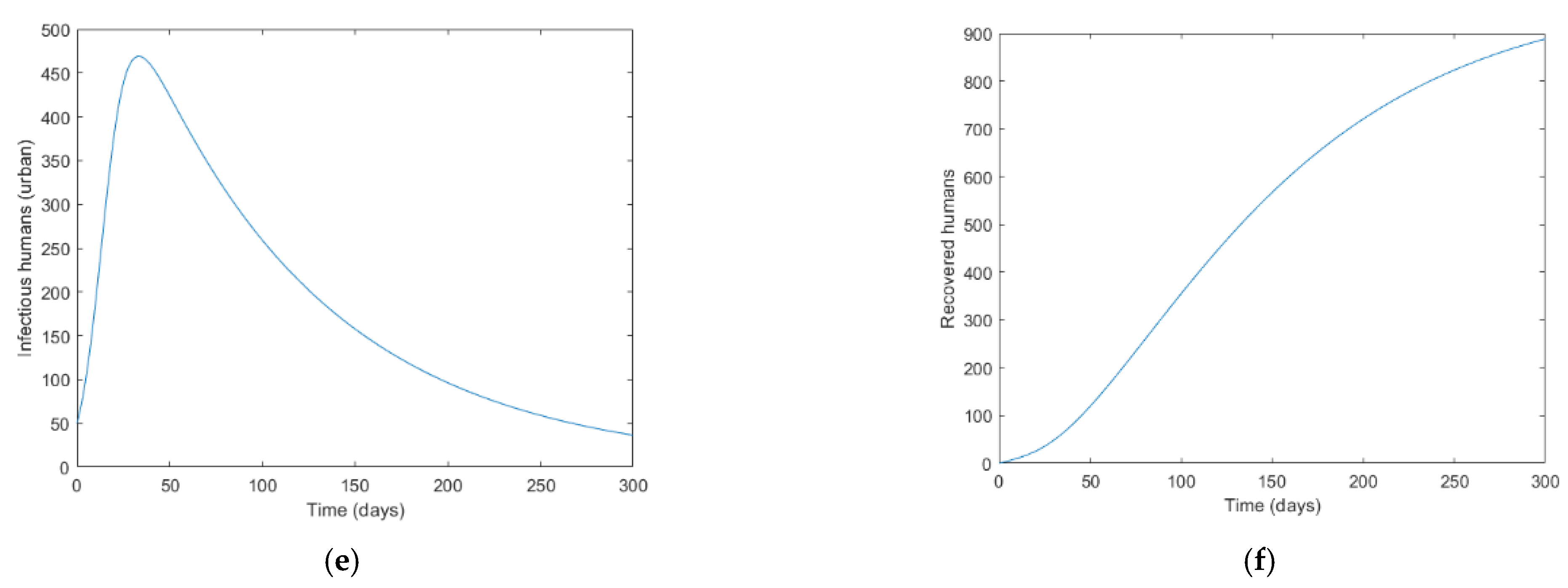
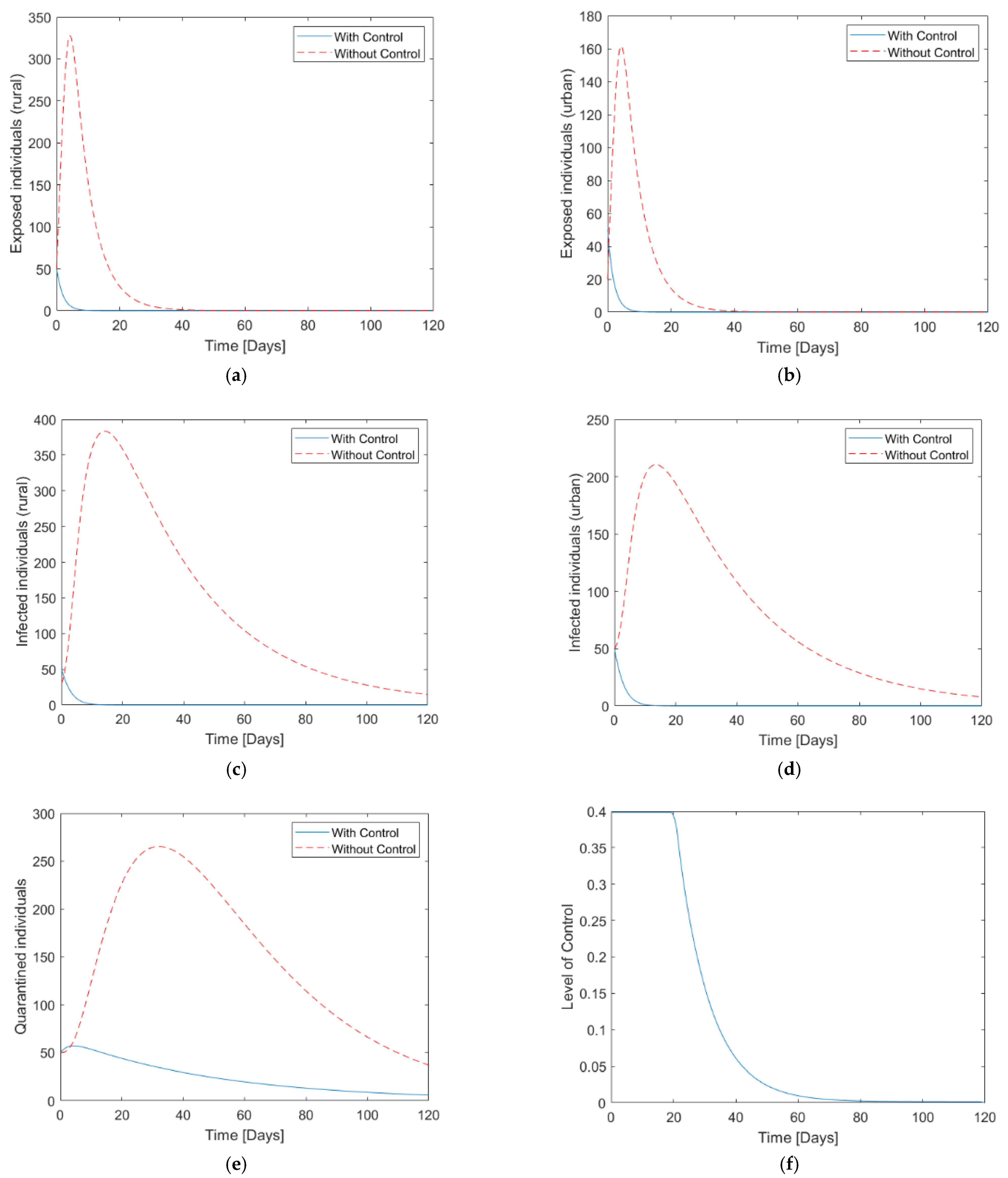
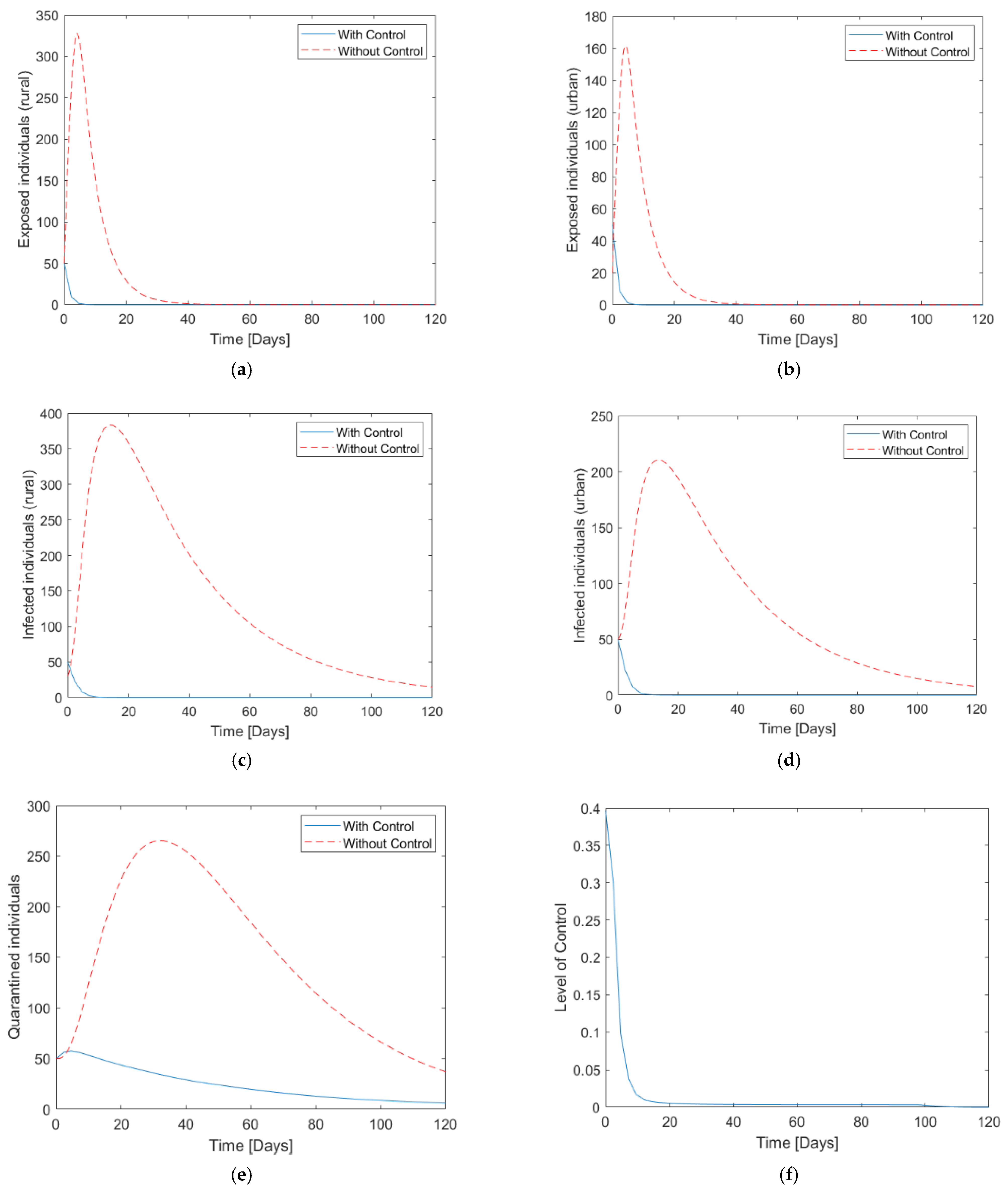
4. Optimal Control Results

This section discusses the numerical analyses for the two control policies in containing the HFMD outbreak. For each policy, the optimality system is solved using the backward/forward sweep method, together with the fourth-order Runge–Kutta integration [53]. In other words, the systems of Equations (5) and (6) are solved through the use of the forward sweep method with a predetermined initial condition, whereas the adjoint equations set forth by Equation (9) are solved using the backward sweep method, subjected to the transversality conditions. To avoid prolonged numerical computations, the ${\beta }_h$ and ${\beta }_l$ parameters are increased tenfold to 0.002 and 0.001, respectively. The other parameters are still the same as given in Table 1. The initial conditions used are the same as for the uncontrolled system described in Section 2.3.

For all simulations, the time t used is fixed at 120 days. The control weights are set at $B_0$ = 1, $B_1$ = 2, $B_2$ = 5. Figure 2 shows the results of applying the control signal u(t) to the system under Policy 1. Note that in practice the control measures cannot be implemented over the entire population, since it is physically impossible to get every member of the human population to vaccinate due to economic viability. In this respect, we set the bounds for both control signals to $u_{max}$ = 0.4. Note that the $u_{max}$ bound will be kept at 0.4 throughout the paper to satisfy the purpose of the paper of investigating the relationship between the time it would take for the control effort to stay at its maximum, against the changes in the control weightings. This will allow the epidemiologists to know beforehand the number of days that a control measure would need to be applied at its maximum possible level before adjusting the measure level. Figure 2a shows the comparison of the responses for the exposed class $E_h$ from the higher outbreak. The $E_h$ response without control exponentially decays to zero around Day 50. The trajectory of $E_h$ with control decays to zero in around Day 10. The infected individuals both for rural ($I_h$) and urban ($I_l$) increases initially without control, though these trajectories all reach zero at around Day 120. The controlled responses for both $I_h$ and $I_l$ exponentially decays to zero at around Day 20. Note that similar controlled trajectories are observed for $I_h$ and $I_l$, even though the uncontrolled responses are different. This is apparent from Equation (6) that the treatment control action is acted on all the exposed and infected classes for both regions (rural and urban) equally, thereby generating similar responses. The level of control is constant at the $u_{max}$ limit for the first 28 days before decaying to zero.

Figure 3 now shows the comparisons between the cases without control, against the cases with control, for the system under the action of Policy 2. The weights used are $B_0$ = 1, $B_1$ = 2, $B_2$ = 1 and $B_3$ = 5. As is seen, the controlled responses for the exposed individuals $E_h$ and $E_l$, and the infected individuals $I_h$ and $I_l$, quickly decay to zero around Day 10. The exposed individuals for both regions follow a similar trend. Both control signals $u_1\left(t\right)$ and $u_2\left(t\right)$ decay to zero within approximately 50 days, which is significantly less than the implementation of only one control, which takes 80 days before reaching zero. This is attributable to the fact that two control measures are used in tandem of one another, thereby eliminating any efforts needed at the upper bound constraint, resulting in reduced number of days of the control administration.

5. Optimal Control Parameters Investigation

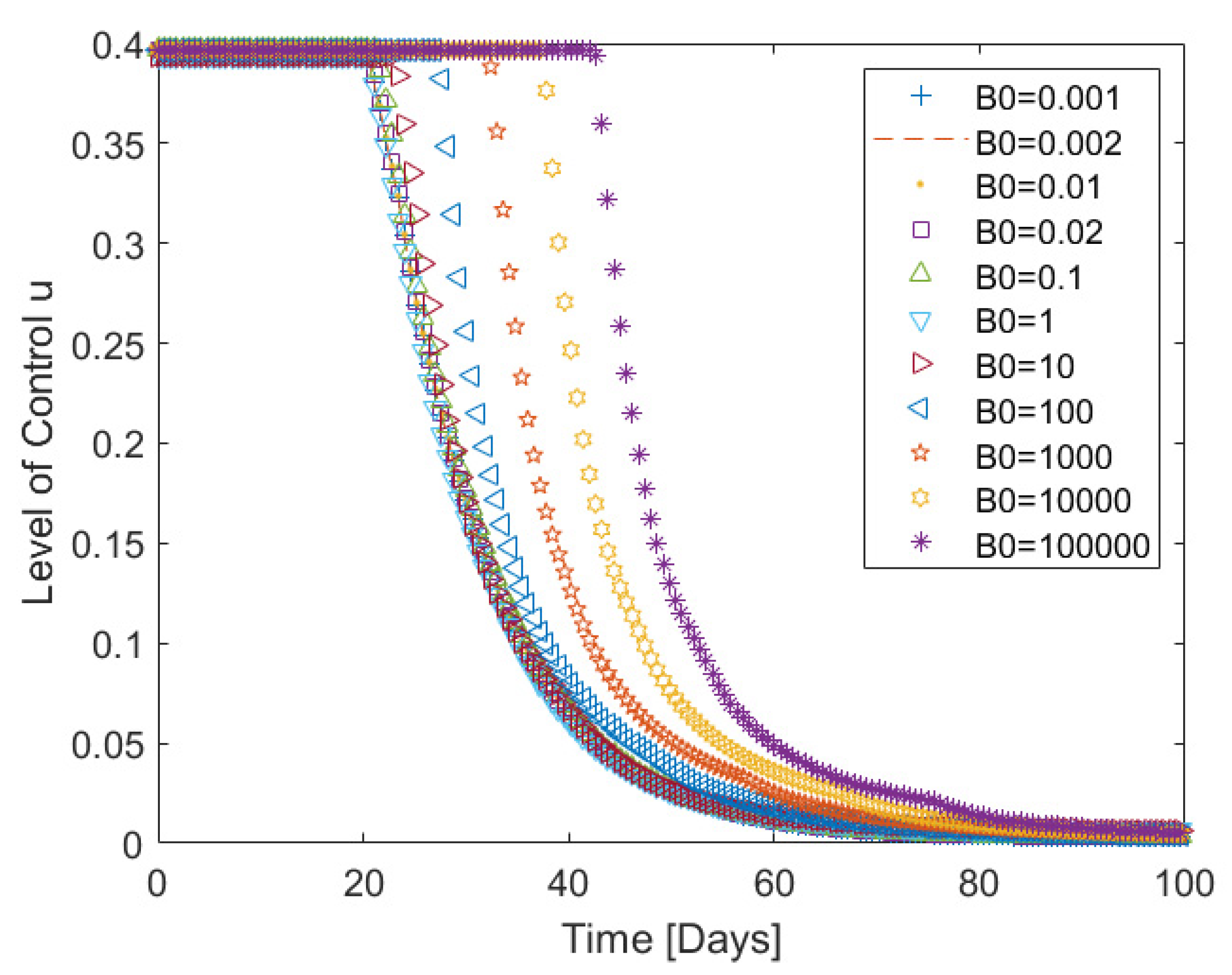
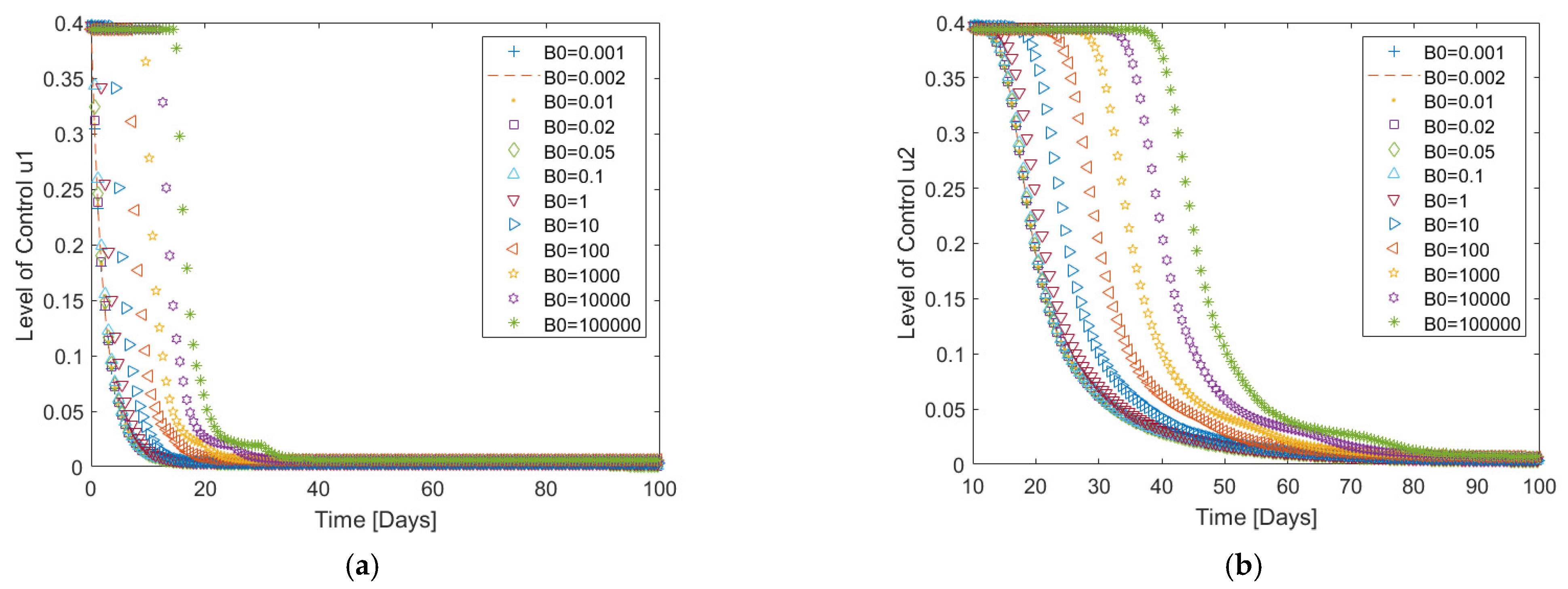
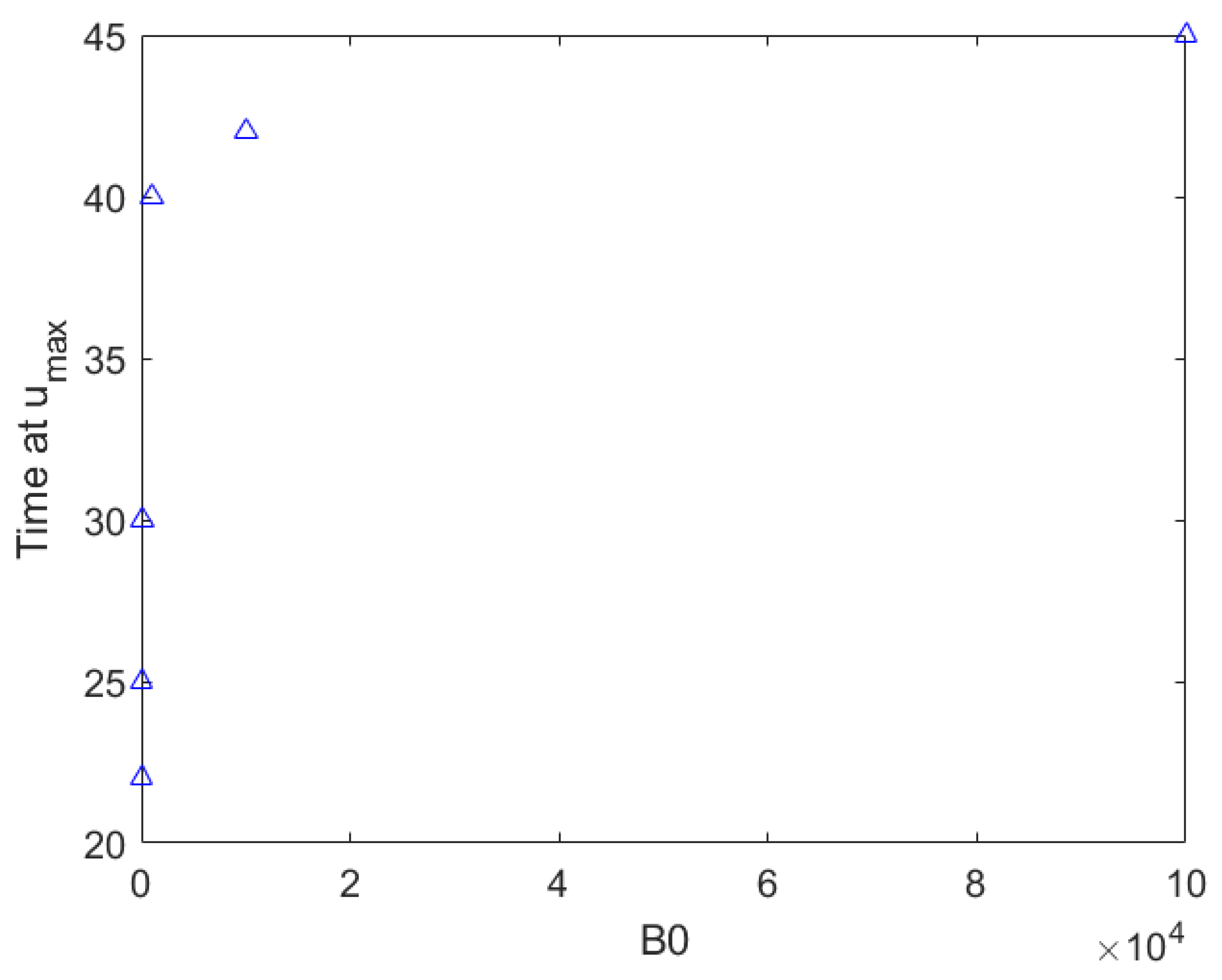
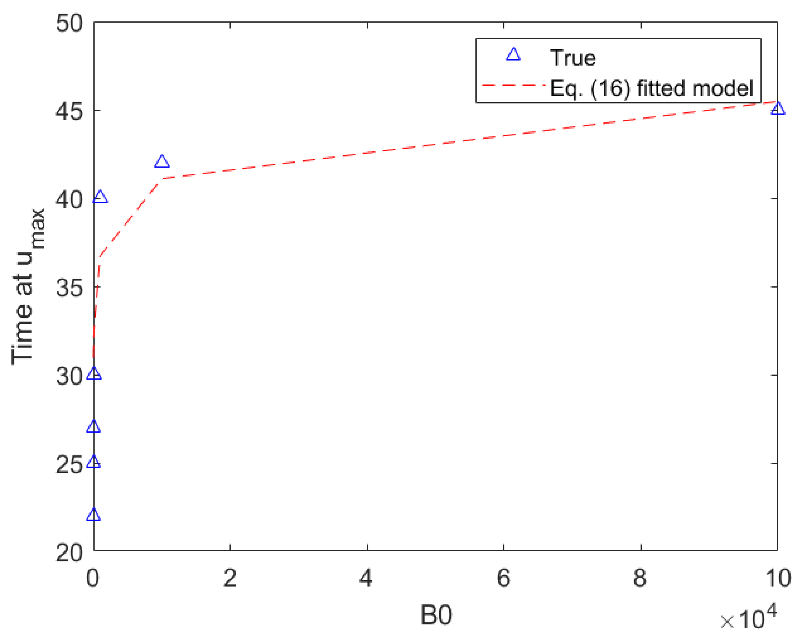
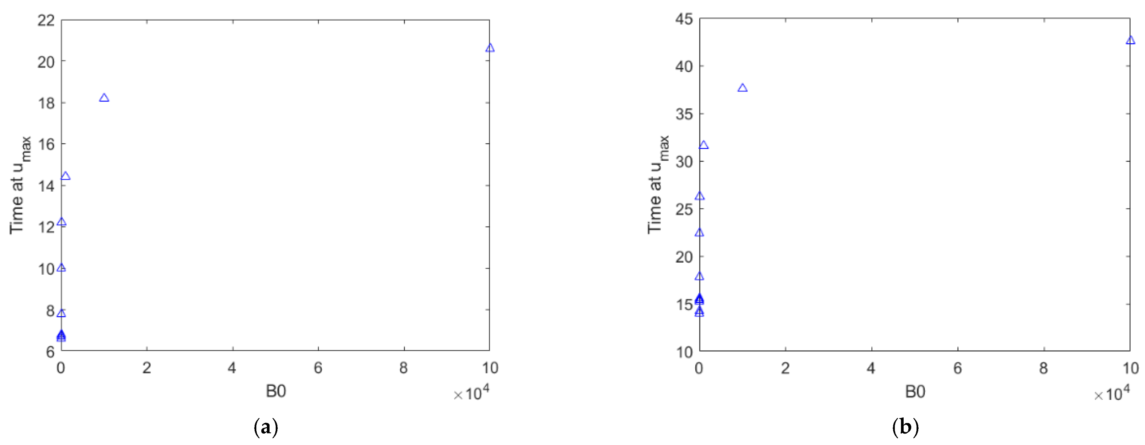
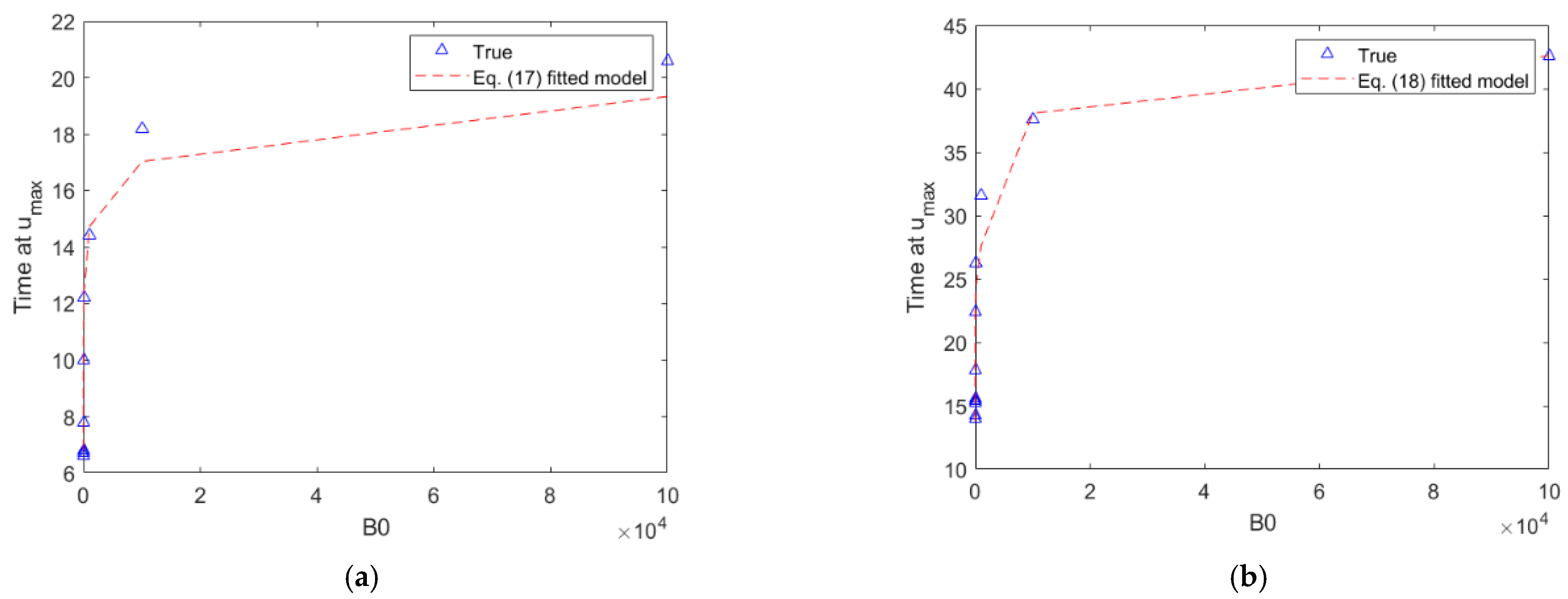
5.1. Changes in B₀ Parameters

To investigate the control system responses to the weight changes in the function of Equation (7) upon the action of Policy 1, the parameter B₀ is first chosen to be the object of investigation. For this, we define the parameter vector as:

$$B_0=[0.001,0.002,0.01,0.02,0.1,1,10,100,1000,\mathrm{10,000},\mathrm{1,000,000}]$$

(15)

This parameter vector captures a wide range of possible $B_0$ weightings, offering numerical insights into the sensitivity of this parameter with respect to changes in $B_0$. For Policy 1, the other weights associating with the functional in Equation (7) are kept constant at $B_1$ = 1 and $B_2$ = 1. The response trajectories are the same as was shown in Figure 2 for all the $B_0$ weightings and thus will not be shown for clarity. Figure 4 plots the required control effort needed to achieve the trajectories of Figure 2. It is apparent from this figure that the general trend for the control effort $u(t)$ is that it stays at $u_{max}$ for a certain time before exponentially decaying to zero. For very small $B_0$ weightings of less than 10 and satisfying $B_0<<B_1$, the control effort is sustained at $u_{max}$ at around 21 days. As $B_0$ increases and becomes significantly greater than $B_1$, that is, from the point of $B_0=100$ onwards, the time spent at $u_{max}$ significantly increases.

To investigate the control system responses to the weight changes in the function of Equation (8) upon the action of Policy 2, for the changes in parameter $B_0$, the parameter vector of Equation (15) is again used, with other weights kept constant at unity throughout the simulation. In this case, the response trajectories are similar to the one depicted in Figure 3. Figure 5 now shows the required control effort needed to achieve the responses of Figure 3. As seen from both subfigures of Figure 5, the general trends for both control efforts are that the control signals stay at the maximum limit $u_{max}$for some time before decaying to zero. For very small $B_0$ weightings, particularly $B_0<<B_1$, the control effort $u_1$ is seen to immediately exponentially decay to zero without staying at the maximum limit $u_{max}$; the control effort $u_2$ is seen to stay at $u_{max}$ for around 20 days before decaying. As $B_0$ increases, particularly satisfying $B_0>>B_1$, the control efforts stay at $u_{max}$ for longer.

A facet of interest in the optimal control design is the ability to predict a priori the time $t_{max}$ required for an optimal control effort to sustain at the constraint $u_{max}$ before exponentially decaying to zero. In terms of the real-world applications, this would mean knowing beforehand the number of days that a control measure would need to be applied at its maximum possible level before adjusting the measure level. This would then allow the relevant authorities to formulate their policies with ease and maximum efficiency. In this respect the time $t_{max}$ needed for the control effort $u(t)$ to stay at $u_{max}$ can be plotted against the values of $B_0$ for the application of Policy 1, as shown in Figure 6.

The plot of Figure 6 suggests a nonlinear relationship in the form of a logarithmic function, which can be written as:

$$t_{max}=\ln (a_1{B}_0+a_2)+a_3$$

(16)

This type of relationship is an intrinsic relationship that can be observed for the optimal control model presented in this paper, as will be observed time and time again with the other parameters $B_1, B_2$ and $B_3$.

The values of the parameters $a_1$, $a_2$ and $a_3$ are determined via nonlinear regression through the command lsqnonlin in Matlab. The $R^2$ value for the match is computed by the method of ref. [54] and was found to be 0.976. Figure 7 shows the match between the model of Equation (16) to the data of Figure 6, validating the logarithmic model. The mean absolute error for the match is 0.4196, which is close to the data of Figure 6.

For Policy 2, the plot of the $t_{max}$ time against the parameters $B_0$ is now plotted in Figure 8. The plot again suggests a similar nonlinear logarithmic relationship to Equation (16) for the function of $t_{max}$ with respect to the changes in $B_0$ for both control inputs $u_1$ and $u_2$. In this respect, the identification of $a_1$, $a_2$ and $a_3$ for the logarithmic model proceeds in the same way as was carried out for Policy 1. The fitted models are:

$$u_1:\hspace{1em}\hspace{1em}\hspace{0.17em}{t}_{\max }=\ln (178.54{ \mathrm{B}}_0+65)+2.59$$

(17)

$$u_2:\hspace{1em}\hspace{1em}\hspace{0.17em}{t}_{max}=\ln (150.54B_0+0.26)+14.71$$

(18)

Figure 9 shows matches between the models of Equations (19) and (20) against the plot of Figure 8. The coefficient of determination for these matches are 0.9869 and 0.9738, respectively. The mean absolute error for the case of $u_1$ is 0.4066, whereas the corresponding mean absolute error for the case of $u_2$ is 1.0603. These matches, along with the coefficients of determination, serve to demonstrate that the logarithmic function is again a good model to describe the control effort change with respect to $B_0$ for both policies.

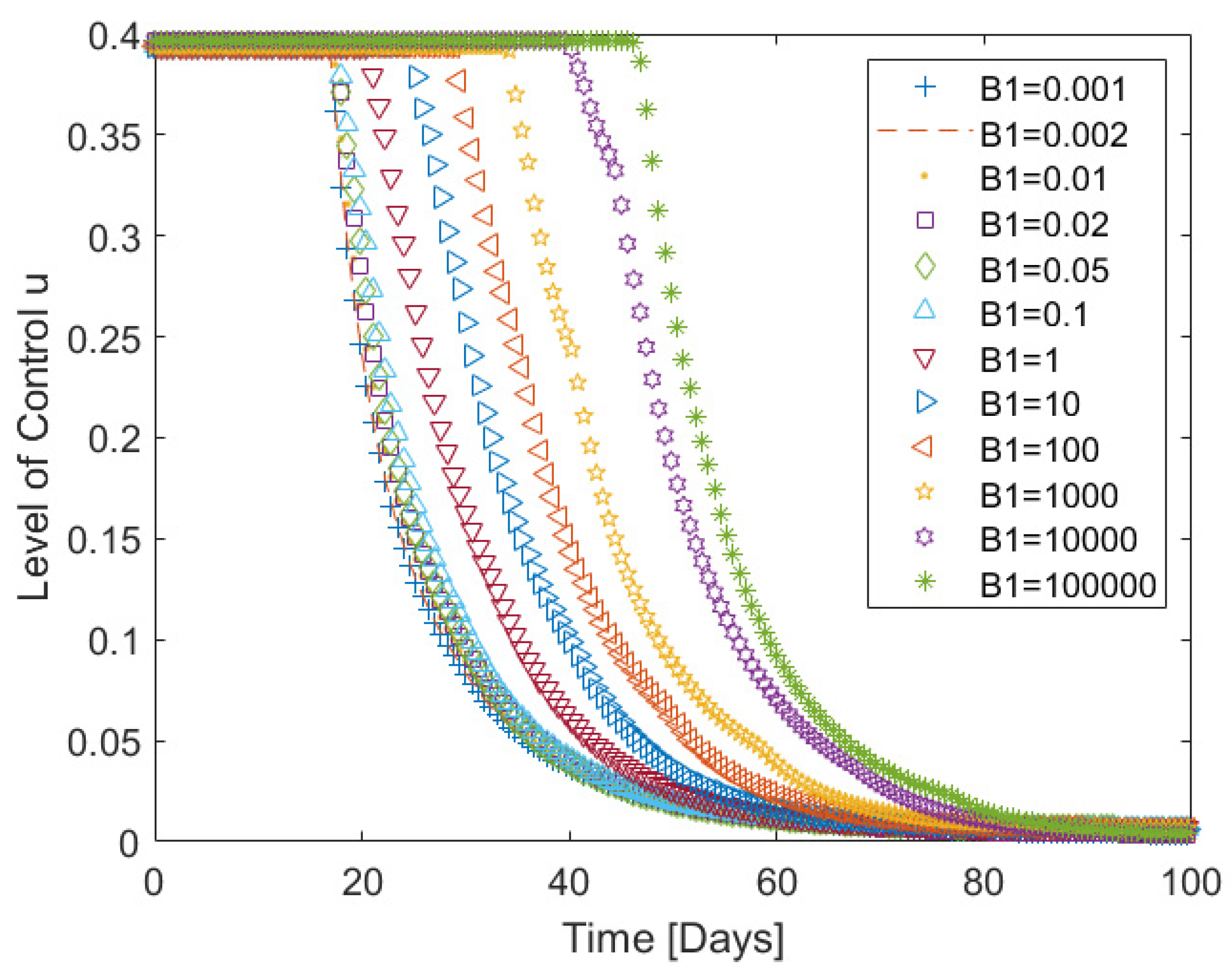
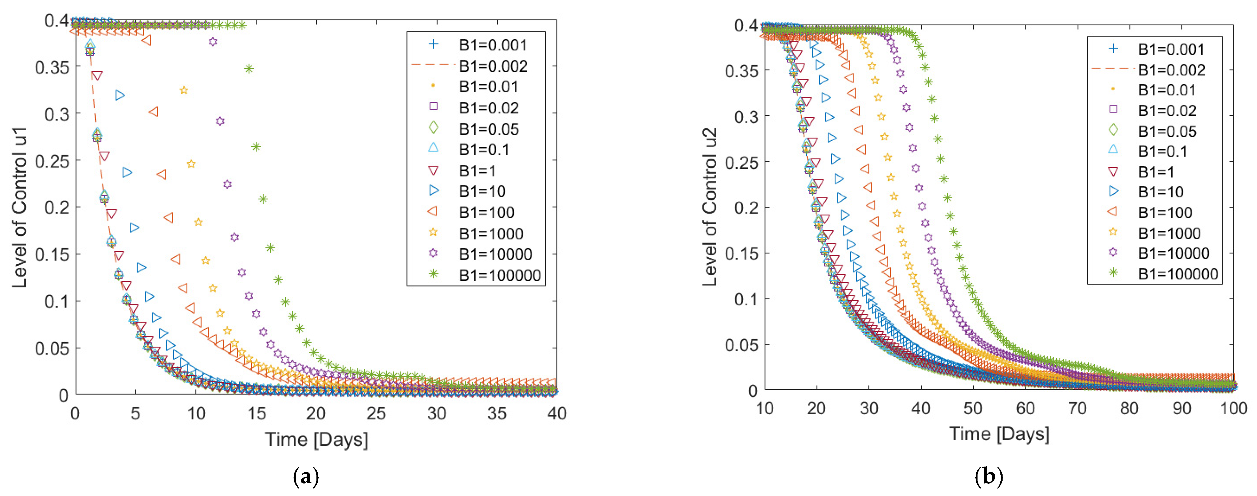
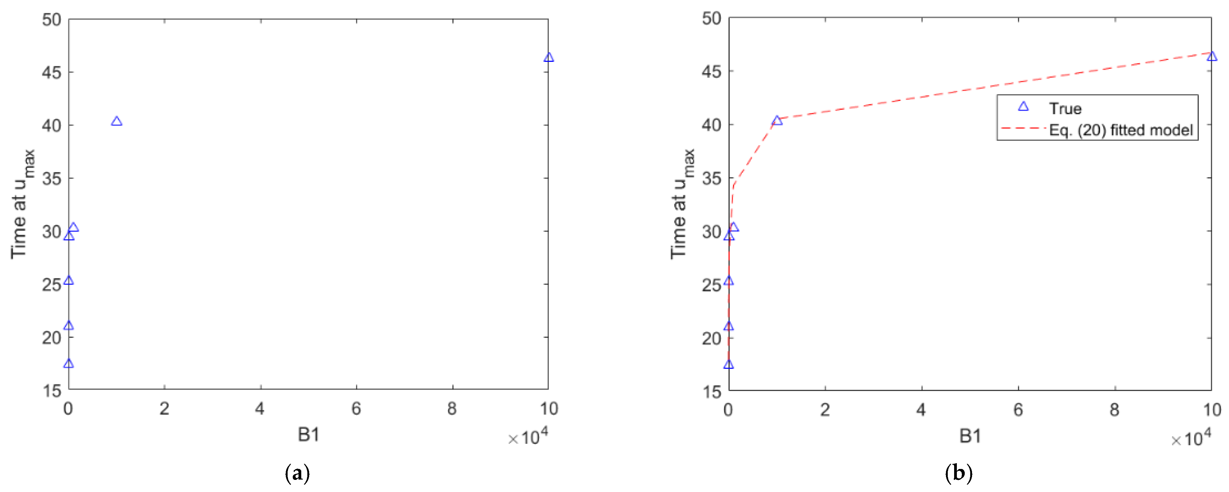
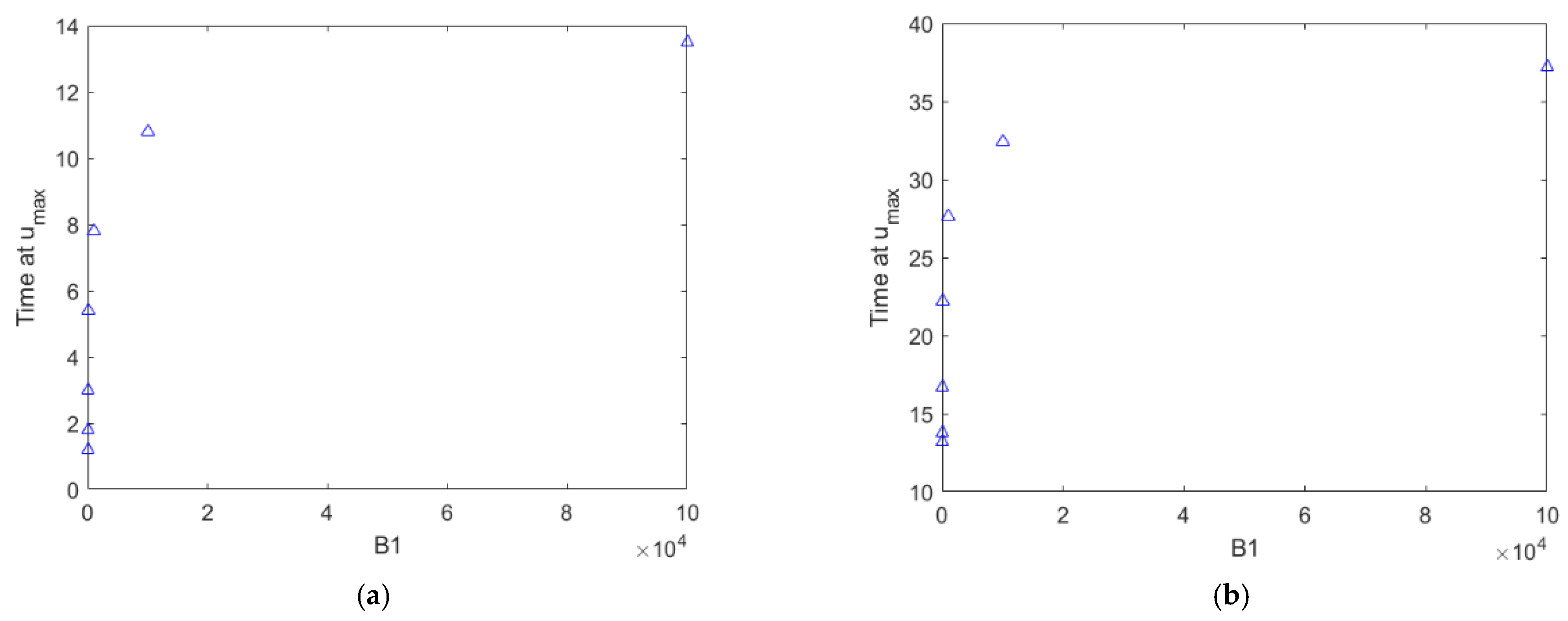
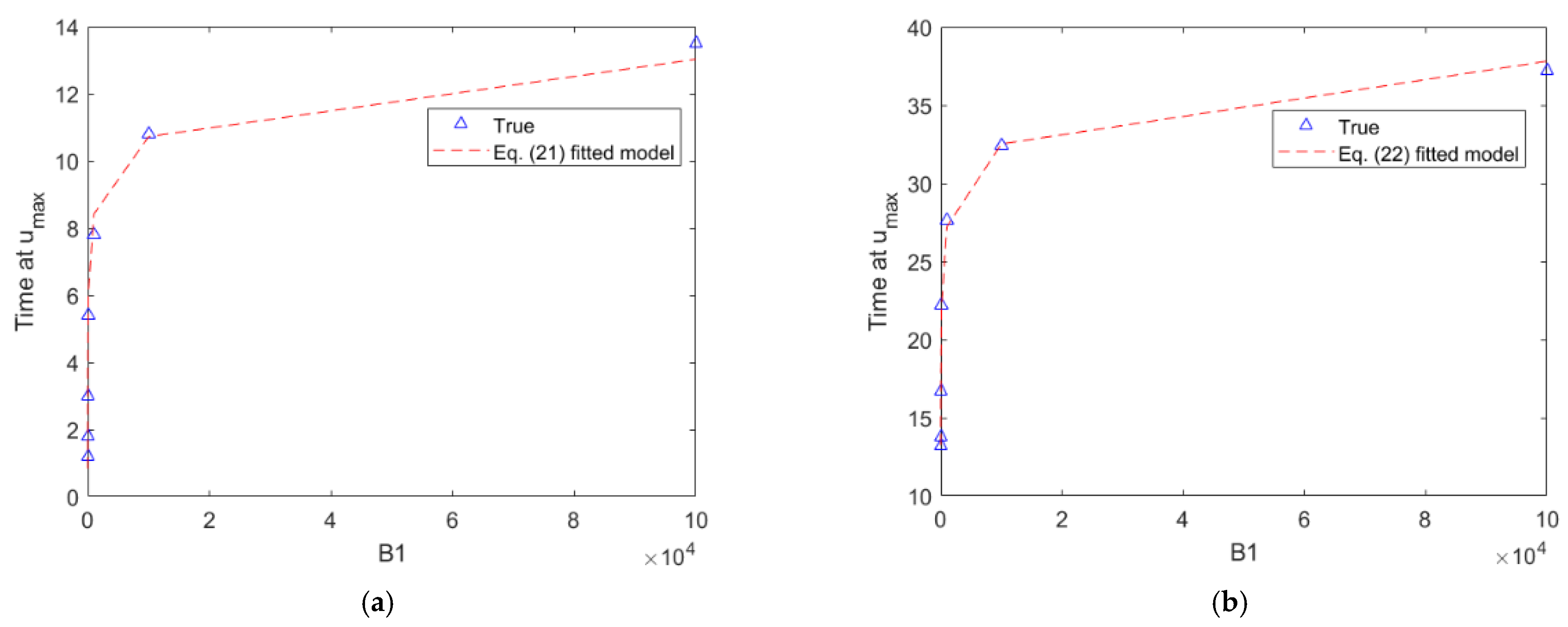
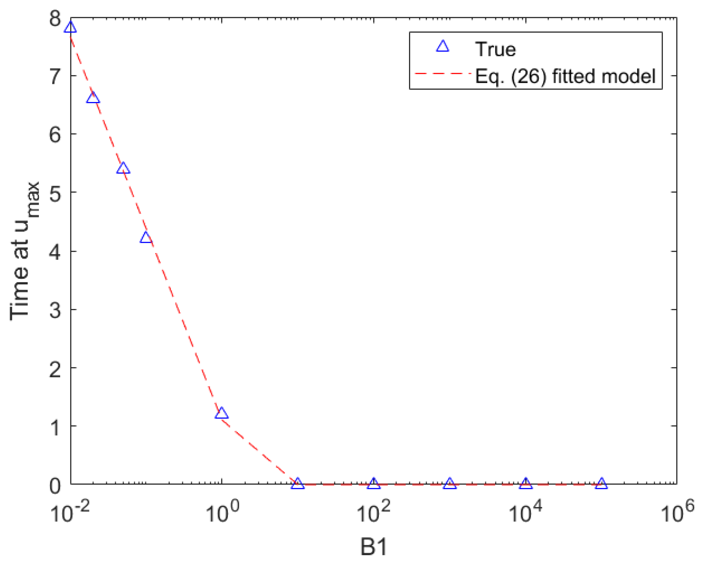
5.2. Changes in B₁ Parameters

To investigate the effects in changing the weights upon the action of Policy 1, the corresponding $B_1$ vector is defined:

$$B_1=[0.001,0.002,0.01,0.02,0.05,0.1,1,10,100,1000,\mathrm{10,000},\mathrm{1,000,000}]$$

(19)

Note that other parameters are kept fixed at unity. The response trajectories are again identical to the one shown in Figure 2. Figure 10 plots the response of the control signal $u(t)$ required to achieve optimal control. It is seen that the increment in $u_{\max }$time is tiny for smaller values of $B_1$ less than 0.1, with greater spacing as $B_1$ is increased.

For the investigation of the effects of changing the $B_1$ weightings on the application of Policy 2 control, the vector of Equation (21) is again used as the $B_1$ weights to be changed. The $B_0, B_2$ and $B_3$ weights are kept constant at unity. Again, the trajectories of the responses are the same as was shown in Figure 3. Figure 11 shows the application of the optimal control efforts. The time needed for the control effort $u_1$ to remain at $u_{\max }$ increases with greater spacings as the value of $B_1$ is changed. In contrast, the time needed for the control effort $u_2$ to stay at $u_{max}$ slightly increases, before reaching the value of about 30 for very large values of $B_1$.

To investigate the $t_{max}$ time further, Figure 12a plots the $t_{max}$ time against $B_1$ for the application of Policy 1. The plot is again in the form of the logarithmic function of Equation (16). Proceeding with the nonlinear regression yields the model:

$$t_{max}=\ln (93.9B_1+942.5)+11.0$$

(20)

which is plotted in Figure 12b in comparison with the data of Figure 12a. The coefficient of determination in this case was 0.9629, whereas the mean absolute error for the match was 1.292, confirming that the match was indeed close to the data of Figure 12a.

For the case of Policy 2, the plot of $t_{max}$ against the parameters $B_1$ is plotted in Figure 13. This plot again suggests a logarithmic relationship in the form of Equation (18) for both control inputs $u_1$ and $u_2$.

The identification of the required parameters proceeded in the same way as was carried out previously. The following models were derived:

$$u_1:\hspace{1em}\hspace{1em}\hspace{0.17em}{t}_{\max }=\ln (14.8{\mathrm{B}}_0+7.6)-1.4$$

(21)

$$u_2:\hspace{1em}\hspace{1em}\hspace{0.17em}{t}_{max}=\ln (20.6B_0+140.9)+8.3$$

(22)

Figure 14 shows matches between the models of Equations (21) and (22) against the plot of Figure 13. The coefficient of determination for the match are 0.9879 and 0.9930, respectively. The mean absolute error for both matches are 0.3931 for the $u_1$ case, and 0.1815 for the $u_2$ case, again confirming the validity of the logarithmic model.

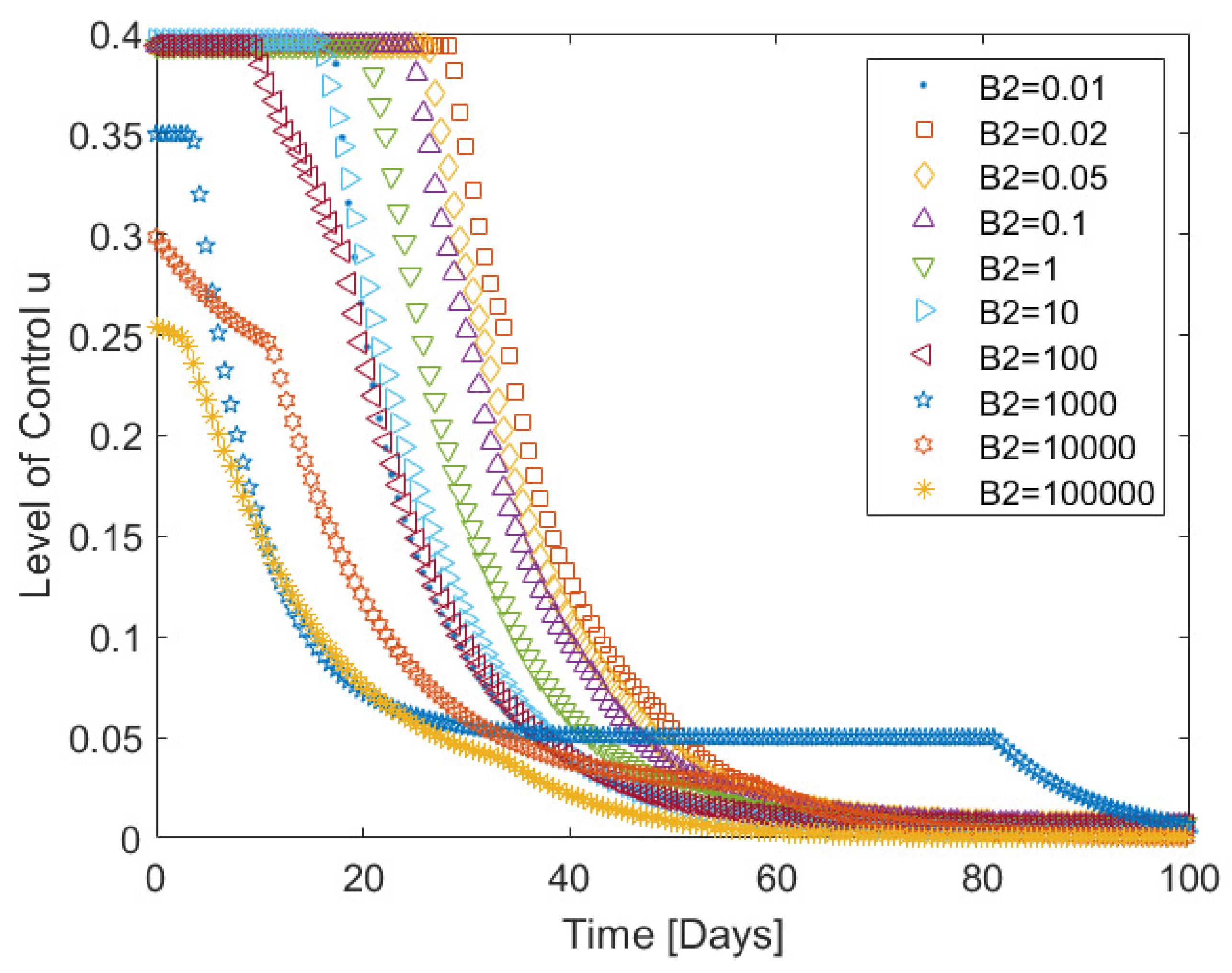
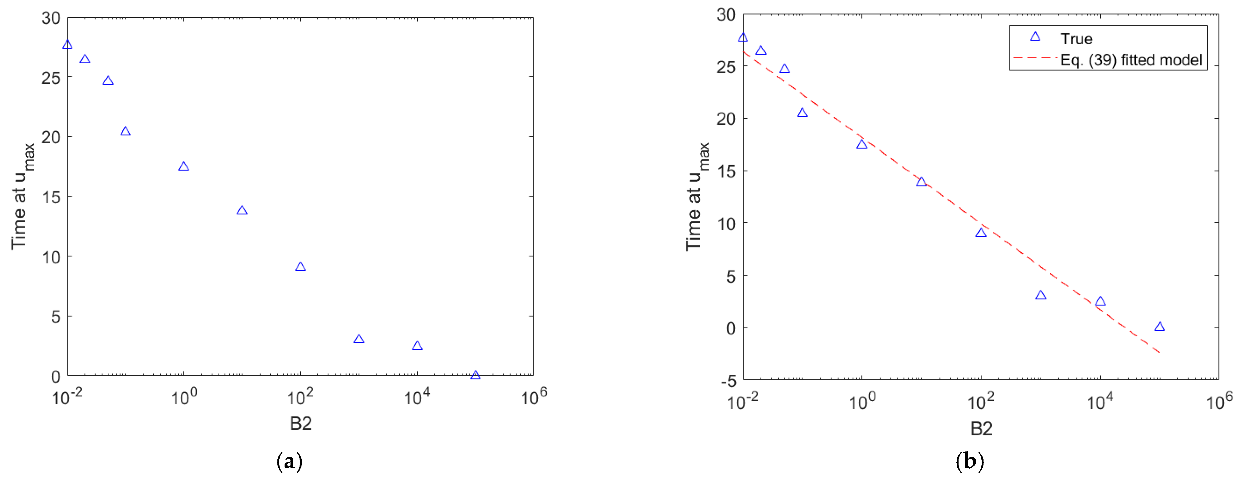
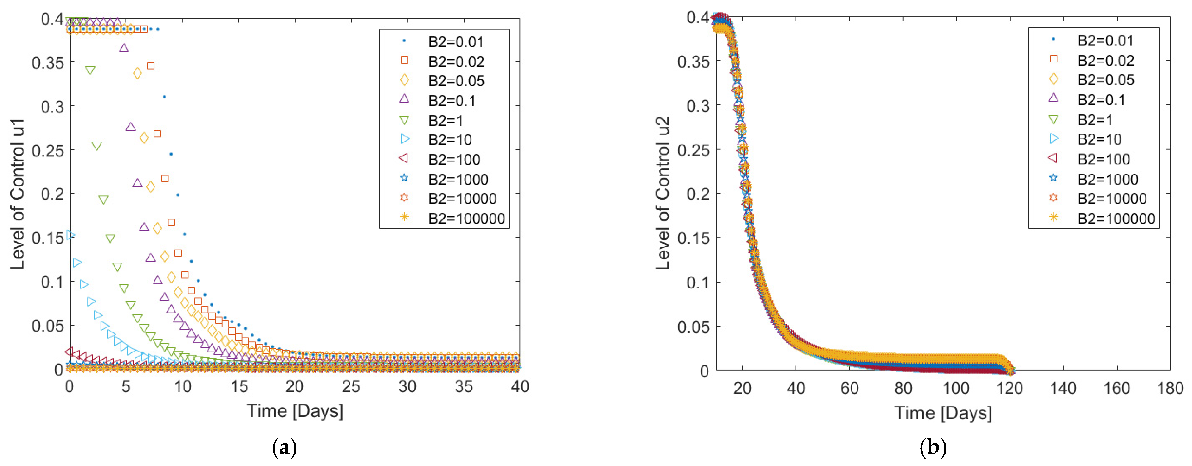
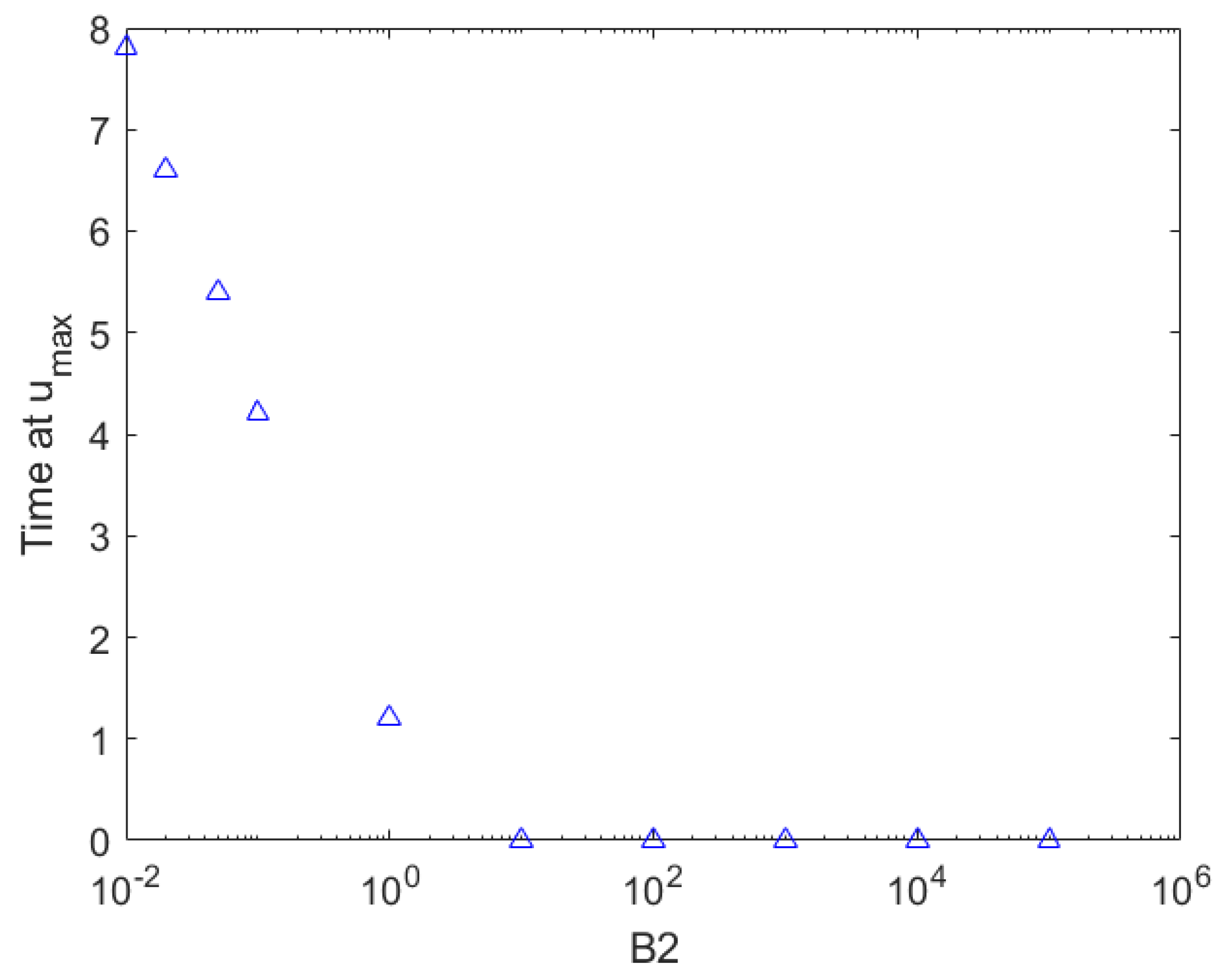
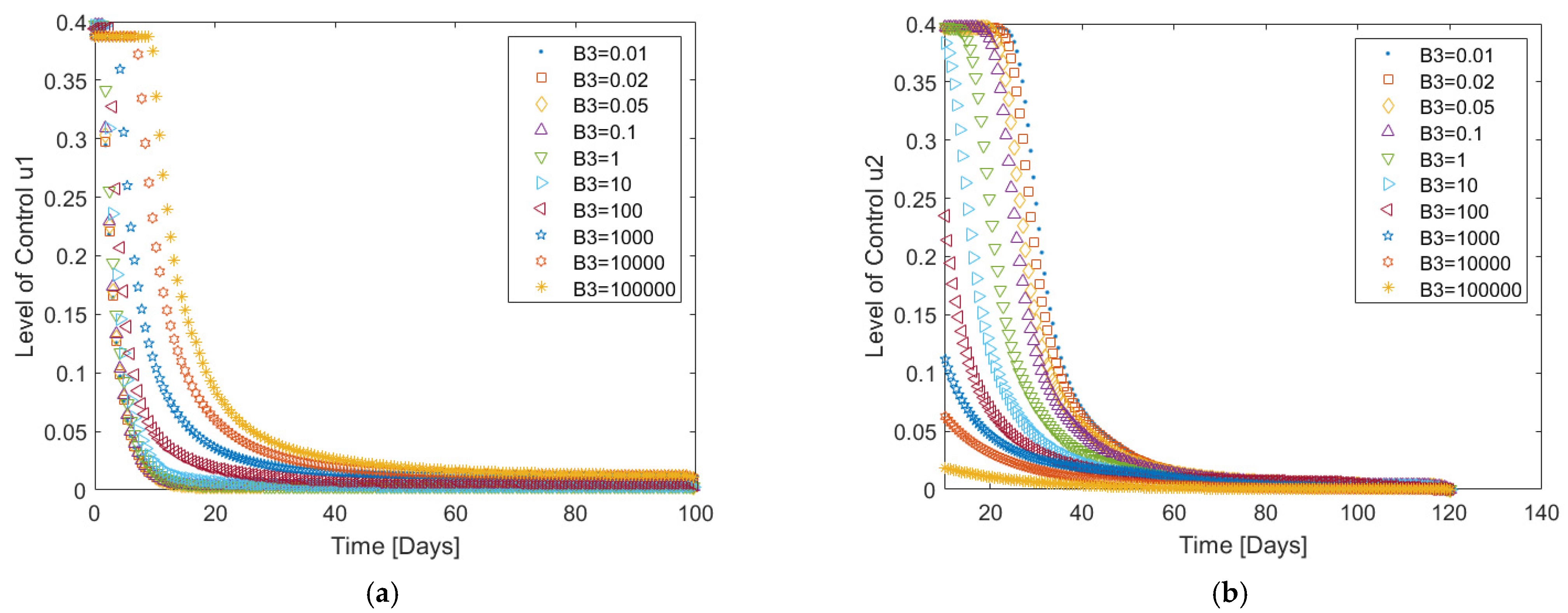
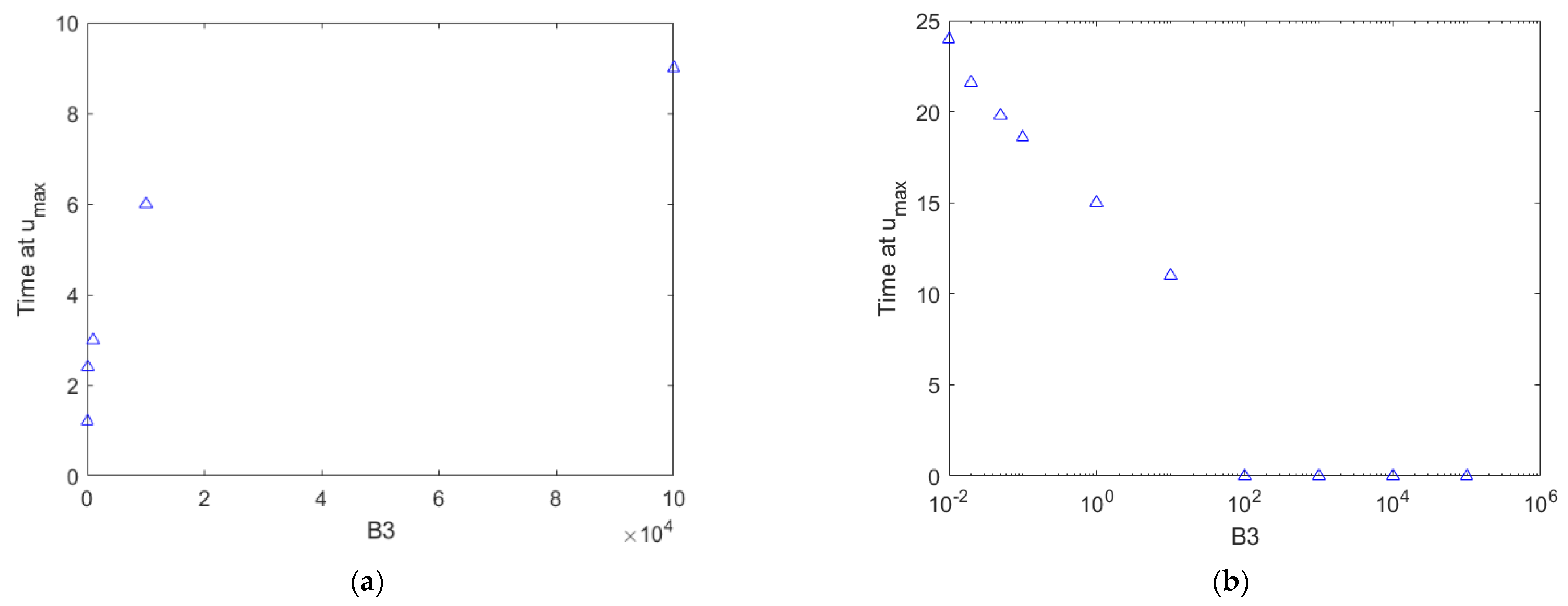
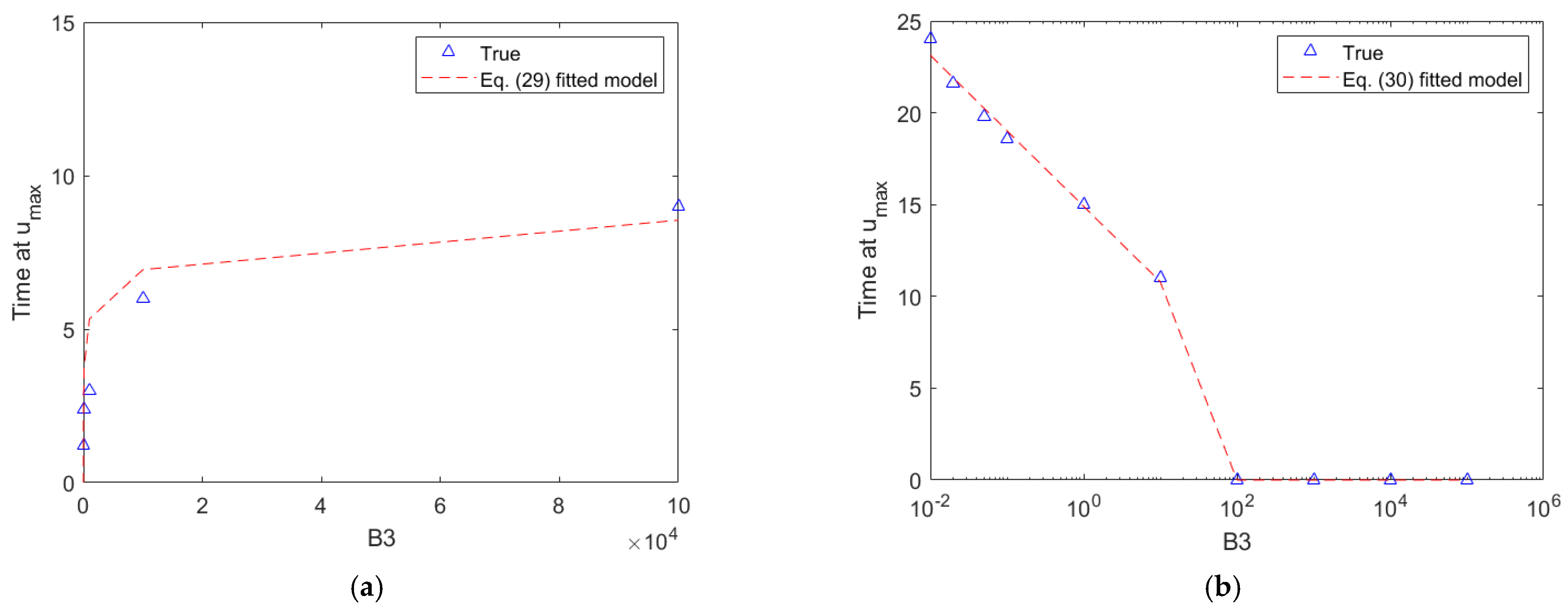
5.3. Changes in the Control Weights

Since the control policies Policy 1 and 2 contain a different number of control parameters, it is possible to investigate the effect of the change in control weights in a few different ways. We begin by considering the case of Policy 1, where there is only the treatment control action. In this respect, we can again define the control weights vector $B_2$:

$$B_2=\left[0.01,0.02,0.05,0.1,1,10,100,1000,1000,\mathrm{100,000}\right]$$

(23)

The other weights, $B_0$ and $B_1$, are kept constant at unity. Figure 15 shows the 310 required control efforts required to achieve optimal control of HFMD, following the application of Policy 1.

It is seen here that as the value of $B_2$ weight increases, the corresponding $t_{\max }$ time decreases. To investigate the rate of increment of this $t_{\max }$ time so that one could form an a priori prediction of the required optimal control effort to implement Policy 1, let us plot the $t_{\max }$ against HFMD below.

It is apparent from Figure 16a that the $t_{\max }$ times appear to be decreasing to zero as weight $B_2$ is increased. Note here that the $B_2$ axis of Figure 16a is in base-10 logarithmic scale for the purpose of clarity. The plotted data is then a straight-line relationship, suggesting the following model:

$$t_{max}=a_1{\log }_{10}{B}_2+a_2$$

(24)

The model of Equation (24) is then identified through the nonlinear regression to be:

$$t_{max}=-4.112{\log }_{10}{B}_2+18.16$$

(25)

The identified model is superimposed onto the data as shown in Figure 16b. The R-squared value of the match is 0.984, whereas the mean absolute error is 0.97, demonstrating that the model was indeed a good fit for the data.

The second case we wish to investigate is the case concerning the application of Policy 2. Since there are two control signals $u_1$ and $u_2$, we would like to investigate the control efforts incurred by these cases in turn. In this light, changing the $B_2$ weightings by the vector given in Equation (25) should be considered. The other parameters are kept constant at $B_0=1,B_1=1$ and $B_3$ = 1. Figure 17 plots the required optimal control efforts to achieve the control of HFMD as weight changes. It is apparent from Figure 17a that the $t_{\max }$times appear to be decreasing to zero as weight $B_2$ is increased for the application of the $u_1$ signal. There is, however, no significant change across the $B_2$ increments for the case of the $u_2$ inputs, as apparent from Figure 17b.

Let us then plot the $t_{max}$ times against the $B_2$ vector Equation (23).

Note that the $B_2$ axis in Figure 18 is in the base-10 logarithmic scale for clarity. Since the plotted data become a straight line up until $B_2$ = 100 and zero thereafter, the relationship between the t_max times against $B_2$ weights is given by a piecewise function as:

$$t_{max}=\{\begin{array}{ll}\alpha {\log }_{10}{B}_2+\beta ,\hfill & \mathrm{for}0.01\le B_2\le 10\hfill \\ 0,\hfill & \mathrm{for}{B}_2>10\hfill \end{array}$$

(26)

The model of Equation (26) is then superimposed onto the plot of Figure 18 as shown in Figure 19, showing an accurate match to the data of Figure 18. Specifically, the mean absolute error between the data and model is 0.0520.

The last case concerning the control parameters is the case where$B_3$ changes. In this respect, let us define the weight vector as:

$$B_3=\left[0.01,0.02,0.05,0.1,1,10,100,1000,1000,100000\right]$$

(27)

The other parameters are kept constant at $B_0$ = 1, $B_1$ = 2, and $B_2$ = 1. Figure 20 plots the required control signals to achieve optimal control of HFMD as the $B_3$ weight changes. It is seen from this figure that, as $B_3$ increases, the t_max time for the control signal $u_1$ increases, whereas the times for the control signal $u_2$ decays to zero.

To establish a relationship between the $t_{max}$ time as a function of the $B_3$ weights, let us now plot $t_{max}$ time against the $B_3$ weights for both control efforts.

Note that Figure 21a is plotted with normal axes, whereas the $B_3$ axis in the plot of Figure 21b is in base-10 logarithmic scale for greater clarity, since the last four values for the $t_{\max }$ times for the control input $u_2$ are zeros. The plot of Figure 21a is a logarithmic function in the form similar to Equation (16) with $B_0$ replaced by $B_3$. The plot of Figure 21b is in the following form:

$$t_{max}=\{\begin{array}{ll}\alpha {\log }_{10}{B}_3+\beta ,\hfill & \mathrm{for}0.01\le B_3\le 100\hfill \\ 0,\hfill & \mathrm{for}{B}_3>100\hfill \end{array}$$

(28)

Equation (28) is in fact similar to the one given in Equation (26), with the difference only being the piecewise range. Nonlinear regression analyses are then performed for both relations, the results being the following model for the $u_1$ signal:

$$t_{max}=\ln (211.30B_3-106.2)+4.86.$$

(29)

The corresponding model for $t_{max}$ data for the $u_2$ control input case is:

$$t_{max}=\{\begin{array}{ll}-4.115{\log }_{10}{B}_3+14.9,\hfill & \mathrm{for}0.01\le B_3\le 100\hfill \\ 0,\hfill & \mathrm{for}{B}_3>100\hfill \end{array}$$

(30)

The models of Equations (29) and (30) are then superimposed onto the plot of Figure 22. It is seen that both models give a close match to the respective data. Numerically the R-squared value for both models are 0.9214 for the case of $u_1$, and 0.99 for the case of $u_2$.

6. Conclusions

This paper has presented the mathematical modeling and control mechanism of the hand, foot and mouth disease (HFMD). The model includes two types of outbreaks, namely higher and lower outbreaks, that give a simplified view of the outbreaks with respect to regional residency. Stability analyses were conducted with standard dynamical systems theories. An optimal control framework was also proposed with respect to two policies, where Policy 1 delimits the use of treatment only, whereas Policy 2 applies vaccination in combination with treatment. Pontryagin’s maximum principle was used to establish necessary and optimal conditions, facilitating optimal control to be developed.

Numerical solutions of the control systems were presented. It was found that, although both controllers were effective in controlling the HFMD outbreaks, their responses were similar to each other, except that the treatment efforts incurred by Policy 2 are substantially reduced in comparison with that required by Policy 1. Investigations were conducted to investigate the control system responses subjected to changes in the weight functions. Numerical results suggest that, as the weights increase, the time required for the controller to stay at the controller limit $u_{max}$ also increases across changes in the control parameters. These phenomena can be predicted a priori effectively using nonlinear models such as the logarithmic model. This ability to predict the most important facets of the optimal controller is vital for an epidemiological controller, as they suggest the cost effectiveness of implementing a controller. Future research directions could look at incorporating economical constraints to the optimal control, as well as investigating the relationship between the $u_{max}$ levels against the parameter weightings.

References

1. World Health Organization. A Guide to Clinical Management and Public Health Response for Hand, Foot and Mouth Disease (HFMD). 2011. Available online: https://iris.wpro.who.int/handle/10665.1/5521 (accessed on 16 January 2020).
2. Wang, M.G.; Sun, H.M.; Liu, X.M.; Deng, X.Q. Clinical analysis of 59 children with hand foot and mouth diseases due to enterovirus EV71 and concomitant viral encephalitis. Euro. Review. Med. Pharm. Sci. 2017, 21, 43–49. [Google Scholar]
3. Chin, S. HFMD: A Disease of Epidemic Proportions? The Asean Post. Available online: https://theaseanpost.com/article/hfmd-disease-epidemic-proportions (accessed on 25 December 2019).
4. D. Bureau of Epidemiology and MoPH: Report on the Situation of Hand, Foot and Mouth Disease (HFMD) in Thailand. Available online: http://www.boe.moph.go.th/boedb/surdata/disease.php?dcontent=old&ds=71 (accessed on 16 January 2020).
5. Puenpa, J.; Auphimai, C.; Korkong, S.; Vongpunsawad, S.; Poovorawan, Y. Enterovirus A71 Infection, Thailand, 2017. Emerg. Infect. Dis. 2018, 24, 1386–1387. [Google Scholar] [CrossRef] [Green Version]
6. D. Bureau of Epidemiology and MoPH: Hand, Foot, and Mouth Disease (HFMD) in Thailand, Situation Update, No. 50. 2017. Available online: https://ddc.moph.go.th/uploads/files/333f54af3da87cf66599a0def2c30856.pdf (accessed on 20 January 2020).
7. D. Bureau of Epidemiology and MoPH: Hand, Foot, and Mouth Disease (HFMD) in Thailand, Situation Update, No. 10. 2019. Available online: http://dcd.ddc.moph.go.th/2016/informations/view/1262 (accessed on 26 May 2020).
8. Ruan, F.; Yang, T.; Ma, H.; Jin, Y.; Song, S.; Fontaine, R.E.; Zhu, B.P. Risk factors for hand, foot, and mouth disease and herpangina and the preventive effect of hand-washing. Pediatrics 2011, 127, e898–e904. [Google Scholar] [CrossRef] [Green Version]
9. Park, S.K.; Park, B.; Ki, M.; Kim, H.; Lee, K.; Jung, C.; Sohn, Y.M.; Choi, S.-M.; Kim, D.-K.; Lee, D.S.; et al. Transmission of seasonal outbreak of childhood enteroviral aseptic meningitis and hand-foot-mouth disease. J. Korean Med. Sci. 2010, 25, 677–683. [Google Scholar] [CrossRef]
10. Chang, L.Y.; King, C.C.; Hsu, K.H.; Ning, H.C.; Tsao, K.C.; Li, C.C.; Huang, Y.C.; Shih, S.R.; Chiou, S.T.; Chen, P.Y.; et al. Risk factors of enterovirus 71 infection and associated hand, foot, and mouth disease/herpangina in children during an epidemic in Taiwan. Pediatrics 2002, 109, e88. [Google Scholar] [CrossRef] [Green Version]
11. Li, Y.; Dang, S.; Deng, H.; Wang, W.; Jia, X.; Gao, N.; Li, M.; Wang, J. Breastfeeding, previous Epstein-Barr virus infection, enterovirus 71 infection, and rural residence are associated with the severity of hand, foot, and mouth disease. Euro. J. Pediatr. 2013, 172, 661–666. [Google Scholar] [CrossRef]
12. Ikai, T.; Yamtree, S.; Takemoto, T.; Tamura, T.; Kanayama, H.; Sato, K.; Kusaka, Y.; Hayashi, H.; Terasawa, H. Medical care ideals among urban and rural residents in Thailand: A qualitative study. Int. J. Equity Health 2016, 15, 2. [Google Scholar] [CrossRef] [PubMed] [Green Version]
13. D. Bureau of Epidemiology and MoPH: Report on the Situation of the Important Communicable Diseases in Region 9. Available online: http://odpc9.ddc.moph.go.th/hot/situlation.htm (accessed on 30 September 2021).
14. Samanta, R. Analysis of a delayed hand foot mouth disease epidemic model with pulse Vaccination. Sys. Sci Contr. Engr. 2014, 2, 61–63. [Google Scholar] [CrossRef]
15. Li, Y.; Zhang, J.; Zhang, X. Modeling and Preventive Measures of Hand, Foot and Mouth Disease (HFMD) in China. Int. J. Environ. Res. Pub. Health 2014, 11, 3108–3117. [Google Scholar] [CrossRef] [PubMed] [Green Version]
16. Zhu, Y.; Xu, B.; Lian, X.; Lin, W.; Zhou, Z.; Wang, W. A Hand-Foot-and-Mouth Disease Model with Periodic Transmission Rate in Wenzhou, China. Abstr. Appl. Anal. 2014, 2014, 1–11. [Google Scholar] [CrossRef]
17. Wu, C. Analysis of a Hand-Foot-Mouth Disease Model with Standard Incidence Rate and Estimation for Basic Reproduction Number, Math. Comput. Appl. 2017, 22, 29. [Google Scholar]
18. Chadsuthi, S.; Wichapeng, S. The Modelling of Hand, Foot, and Mouth Disease in Contaminated Environments in Bangkok, Thailand. Comput. Math. Methods Med. 2018, 2018, 5168931. [Google Scholar] [CrossRef] [PubMed] [Green Version]
19. Tan, H.; Cao, H. The Dynamics and Optimal Control of a Hand-Foot-Mouth Disease Model. Comput. Math. Methods Med. 2018, 2018, 9254794. [Google Scholar] [CrossRef] [PubMed]
20. Wang, P.; Zhao, H.; You, F.; Zhou, H.; Goggins, W.B. Seasonal modeling of hand, foot and mouth disease as a function of meteorological variations in Chongqink, China. Int. J. Biometeorol. 2017, 61, 1411–1419. [Google Scholar] [CrossRef]
21. Ghanbari, B. On approximate solutions for a fractional prey-predator model involving the Atangana-Baleanu derivative. Adv. Differ. Equ. 2020, 679. [Google Scholar] [CrossRef]
22. Ghanbari, B. On the modeling of the interaction between tumor growth and the immune system using some new fractional and fractional-fractal operators. Adv. Differ. Equ. 2020, 585. [Google Scholar] [CrossRef]
23. Ghanbari, B. A fractional system of delay differential equation with nonsingular kernels in modeling hand-foot-mouth disease. Adv. Differ. Equ. 2020, 536. [Google Scholar] [CrossRef]
24. Rahman, G.; Nisar, K.S.; Ghanbari, B.; Abdeljawad, T. On generalized fractional integral inequalities for the monotone weighted Chebyshev functionals. Adv. Differ. Equ. 2020, 368. [Google Scholar] [CrossRef]
25. Ghanbari, B.; Kumar, S. A study on fractional predator-prey-pathogen model with Mittag-Leffler kernel-based operators. Numer. Methods Partial Differ. Equ. 2020. [Google Scholar] [CrossRef]
26. Ghanbari, B. Mathematical and numerical analysis of a three-species predator-prey model with herd behavior and time fractionalorder derivative. Math. Method Appl. Sci. 2020, 43, 1736–1752. [Google Scholar] [CrossRef]
27. Munusamy, K.; Ravichandran, C.; Nisar, K.S. Existence of solutions for some functional integrodifferential equations with nonlocal conditions. Math. Method Appl. Sci. 2020, 43, 10319–10331. [Google Scholar] [CrossRef]
28. Ghanbari, B. On forecasting the spread of the COVID-19 in Iran: The second wave. Chaos Solitons Fractals 2020, 140, 110176. [Google Scholar] [CrossRef]
29. Djilali, S.; Ghanbari, B. Coronavirus pandemic: A predictive analysis of the peak outbreak epidemic in South Africa, Turkey, and Brazil. Chaos Solitons Fractals 2020, 138, 109971. [Google Scholar] [CrossRef]
30. Bichara, D.; Kang, Y.; Castillo-Chavez, C.; Horan, R.; Perrings, C. SIS and SIR epidemic models under virtual dispersal. Bull. Math. Biol. 2015, 77, 2004–2034. [Google Scholar] [CrossRef]
31. Castillo-Chavez, C.; Bichara, D.; Morin, B.R. Perspectives on the role of mobility, behavior, and time scales in the spread of diseases. Proc. Natl. Acad. Sci. USA 2016, 113, 14582–14588. [Google Scholar] [CrossRef] [Green Version]
32. Moreno, V.; Espinoza, B.; Barley, K.; Paredes, M.; Bichara, D.; Mubayi, A.; Castillo-Chavez, C. The role of mobility and health disparities on the transmission dynamics of Tuberculosis. Theor. Biol. Med. Model. 2017, 14, 3. [Google Scholar] [CrossRef]
33. Lolika, P.O.; Mushayabasa, S. On the Role of Short-Term Animal Movements on the Persistence of Brucellosis. Mathematics 2018, 6, 154. [Google Scholar] [CrossRef] [Green Version]
34. Rodrigues, H.S.; Monteiro, M.T.; Torres, D.F.M. Dynamics of Dengue epidemics when using optimal control. Math. Comput. Model. 2010, 52, 1667–1673. [Google Scholar] [CrossRef] [Green Version]
35. Pongsumpun, P.; Tang, I.M.; Wongvanich, N. Optimal control of the dengue dynamical transmission with vertical transmission. Adv. Differ. Equ. 2019, 2019, 176. [Google Scholar] [CrossRef] [Green Version]
36. Imran, M.; Usman, M.; Malik, T.; Ansari, A.R. Mathematical analysis of the role of hospitalization/isolation in controlling the spread of Zika fever. Virus Res. 2018, 255, 95–104. [Google Scholar] [CrossRef]
37. Momoh, A.A.; Fuegenschuh, A. Optimal control of intervention strategies and cost effectiveness analysis for a Zika virus model. Oper. Res. Health Care 2018, 18, 99–111. [Google Scholar] [CrossRef]
38. Gonzalez-Parra, G.; Díaz-Rodríguez, M.; Arenas, A.J. Mathematical modeling to design public health policies for Chikungunya epidemic using optimal control. Optim. Control. Appl. Methods 2020, 41, 1584–1603. [Google Scholar] [CrossRef]
39. González-Parra, G.; Díaz-Rodríguez, M.; Arenas, A.J. Optimization of the Controls against the Spread of Zika Virus in Populations. Computation 2020, 8, 76. [Google Scholar] [CrossRef]
40. Okyere, E.; De-Graft Ankamah, J.; Hunkpe, A.K.; Mensah, D. Deterministic epidemic models for ebola infection with time-dependent controls. Discrete. Dyn. Nat. Soc. 2020, 2020, 2823816. [Google Scholar] [CrossRef]
41. Wongvanich, N.; Boksuwan, S.; Chesof, A. Simplified modelling and backstepping control of the long arm agricultural rover. Adv. Differ. Equ. 2020, 2020, 701. [Google Scholar] [CrossRef]
42. The Thailand Primary Health Care Division. Available online: http://www.thaiphc.net (accessed on 30 May 2021). (In Thai).
43. Chanprasopchai, P.; Ming-tang, I.; Pongsumpun, P. SIR Model for Dengue Disease with Effect of Dengue Vaccination. Comput. Math. Methods Med. 2018, 2018, 9861572. [Google Scholar] [CrossRef]
44. Chanprasopchai, P.; Pongsumpun, P.; Tang, I.M. Effect of Rainfall for the Dynamical Transmission Model of the Dengue Disease in Thailand. Comput. Math. Methods Med. 2017, 2017, 2541862. [Google Scholar] [CrossRef]
45. Herdicho, F.F.; Chukwu, W.; Tasman, H. An optimal control of malaria transmission model with mosquito seasonal factor. Results Phys. 2021, 25, 104238. [Google Scholar]
46. The World Bank. Life Expectancy at Birth, Total (Years)—Thailand. Available online: https://data.worldbank.org/indicator/SP.DYN.LE00.IN?locations=TH&view=chart (accessed on 26 May 2020).
47. Yang, Z.; Zhang, Q.; Cowling, B.J.; Lau, E.H. Estimating the incubation period of hand, foot and mouth disease for children in different age groups. Sci. Rep. 2017, 7, 16464. [Google Scholar] [CrossRef]
48. Guan, X.; Che, Y.; Wei, S.; Li, S.; Zhao, Z.; Tong, Y.; Wang, L.; Gong, W.; Zhang, Y.; Zhao, Y.; et al. Effectiveness and safety of an inactivated Enterovirus 71 vaccines in children aged 6–71 months in a phase IV study. Clin. Infect. Dis. 2019, 71, 2421–2427. [Google Scholar] [CrossRef]
49. Yang, Z.; Gao, F.; Wang, X.; Shi, L.; Zhou, Z.; Jiang, Y.; Ma, X.; Zhang, C.; Zhou, C.; Zeng, X.; et al. Development and characterization of an enterovirus 71 (EV-71) virus-like particles (VLPs) vaccines produced in Pichia pastoris. Hum. Vaccin. Immunother. 2019, 16, 1602–1610. [Google Scholar] [CrossRef]
50. Jiang, L.; Fan, R.; Sun, S.; Fan, P.; Su, W.; Zhou, Y.; Gao, F.; Xu, F.; Kong, W.; Jiang, C.; et al. A new EV71 VP3 epitope in novovirus P particle vector displays neutralizing activity and protection in vivo in mice. Vaccine 2015, 33, 6596–6603. [Google Scholar] [CrossRef]
51. Fleming, W.H.; Richel, R.W. Deterministic and Stochastic Optimal Control; Springer: New York, NY, USA, 1975; Volume 1. [Google Scholar]
52. Lukes, D.L. Differential Equations Electronics Resource: Classical to Controlled; Elsevier: Amsterdam, The Netherlands, 1982. [Google Scholar]
53. Lenhart, S.; Workman, J.T. Optimal Control Applied to Biological Models; CRC Press: Boca Roton, FL, USA, 2007. [Google Scholar]
54. Dufour, J.M. Coefficient of Determination. Available online: https://jeanmariedufour.github.io/ResE/Dufour_1983_R2_W.pdf (accessed on 30 May 2021).
Figure 1. Numerical simulation for the endemic equilibrium case with the parameters shown in Table 1 and parameters of Equation (1). (a) Susceptible individuals S; (b) Exposed individuals (rural) E h ; (c) Exposed individuals (urban) E l ; (d) Infected individuals (rural) I h ; (e) Infected individuals (urban) I l ; (f) Recovered individuals R .
Mathematics 09 02863 g001aMathematics 09 02863 g001b
Figure 2. Comparisons between the cases without control and with control under the action of Policy 1: (a) Exposed individuals (rural) Eh; (b) Exposed individuals (rural) E h ; (c) Exposed individuals (urban) E l ; (d) Infected individuals (rural) I h ; (e) Infected individuals (urban) I l ; (f) Control effort u ( t ) .
Mathematics 09 02863 g002
Figure 3. Comparisons between the cases without control and with control under the action of Policy 2: (a) Exposed individuals (rural) Eh; (b) Exposed individuals (rural) E h ; (c) Exposed individuals (urban) E l ; (d) Infected individuals (rural) I h ; (e) Infected individuals (urban) I l ; (f) Control effort u 1 ( t ) ; (g) Control effort u 2 ( t ) .
Mathematics 09 02863 g003aMathematics 09 02863 g003b
Figure 4. The control efforts u of Policy 1 against the changes in B 0 weightings of Equation (15).
Mathematics 09 02863 g004
Figure 5. The control efforts u 1 and u 2 of Policy 2 against the changes in B 0 of Equation (15). (a) Control effort u 1 ; (b) Control effort u 2 .
Mathematics 09 02863 g005
Figure 6. The t m a x time of Policy 1 against the changes in B 0 of Equation (15).
Mathematics 09 02863 g006
Figure 7. The t m a x time of Policy 1 against the changes in B 0 of Equation (15), against the fitted model of Equation (16).
Mathematics 09 02863 g007
Figure 8. The t m a x time of Policy 2 against the changes in B 0 of Equation (15). (a) Control effort u 1 ; (b) Control effort u 2 .
Mathematics 09 02863 g008
Figure 9. The t m a x time of Policy 2 against the changes in B 0 of Equation (15), versus the fitted models of Equations (17) and (18). (a) Control effort u 1 ; (b) Control effort u 2 .
Mathematics 09 02863 g009
Figure 10. The level of control effort u ( t ) against the changes in B 1 of Equation (19).
Mathematics 09 02863 g010
Figure 11. The control efforts u 1 and u 2 of Policy 1 against the changes in B 1 of Equation (19). (a) Control effort u 1 ; (b) Control effort u 2 .
Mathematics 09 02863 g011
Figure 12. The t m a x time against parameters B 1 for the application of Policy 1. (a) The t m a x time against parameters B 1 (b) The t m a x time against parameters B 1 , versus the fitted model.
Mathematics 09 02863 g012
Figure 13. The t m a x time against parameters B 1 for the application of Policy 2. (a) Control effort u 1 ; (b) Control effort u 2 .
Mathematics 09 02863 g013
Figure 14. The t m a x time against parameters B 1 for the application of Policy 2 versus the fitted model of Equations (21) and (22). (a) Control effort u 1 ; (b) Control effort u 2 .
Mathematics 09 02863 g014
Figure 15. The time required for control signal u to stay at its maximum, t m a x , against the parameters of Equation (23).
Mathematics 09 02863 g015
Figure 16. The t m a x time against parameters B 2 for the application of Policy 1: (a) The t m a x time against parameters B2; (b) the t m a x time against parameters B2, versus the fitted model.
Mathematics 09 02863 g016
Figure 17. The t m a x time against parameters B 2 for the application of Policy 1 (a) The t m a x time against parameters B2; (b) the t m a x time against parameters B2, versus the fitted model.
Mathematics 09 02863 g017
Figure 18. The control effort u 1 under the change of B 2 in Policy 2.
Mathematics 09 02863 g018
Figure 19. The time required for control signal u ( t ) to stay at its maximum, t m a x , against the parameters of Equation (23).
Mathematics 09 02863 g019
Figure 20. The control efforts required for the application of Policy 2 with respect to changes in B 3 . (a) Control effort u 1 ; (b) Control effort u 2 .
Mathematics 09 02863 g020
Figure 21. The t m a x times required for both control efforts in the application of Policy 3, for the change of B3 weightings of Equation (27). (a) Control effort u 1 ; (b) Control effort u 2 .
Mathematics 09 02863 g021
Figure 22. The t m a x times required for both control efforts in the application of Policy 3, for the change of B3 weightings of Equation (27). (a) Control effort u 1 ; (b) Control effort u 2 .
Mathematics 09 02863 g022