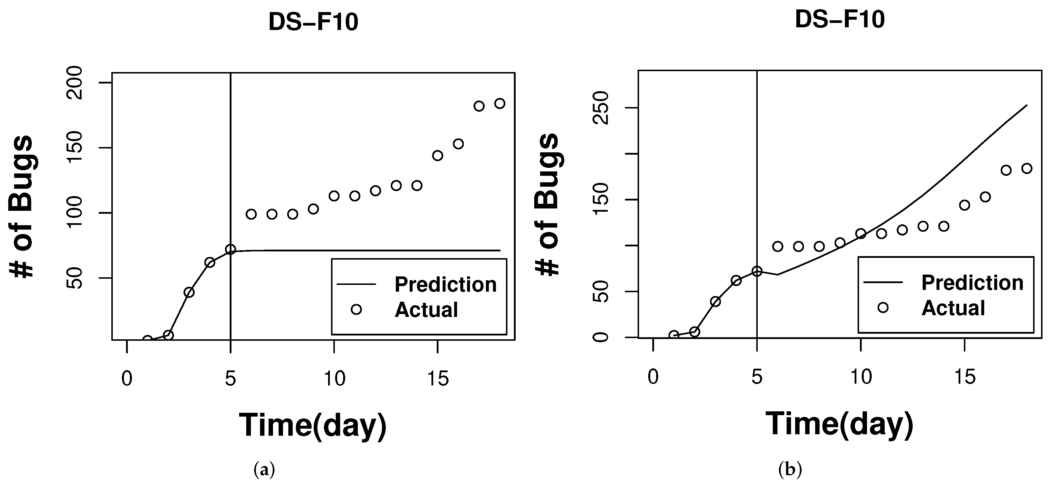
Article

Deep Cross-Project Software Reliability Growth Model Using Project Similarity-Based Clustering

1
Department of Computer Science and Engineering, Waseda University, Shinjuku-ku, Tokyo 169-8555, Japan
2
Department of Information Systems, Osaka Institute of Technology, Hirakata City, Osaka 573-0196, Japan
3
e-Seikatsu Co., Ltd., Minato-ku, Tokyo 106-0047, Japan
*
Author to whom correspondence should be addressed.
Submission received: 16 October 2021 / Revised: 9 November 2021 / Accepted: 10 November 2021 / Published: 18 November 2021
(This article belongs to the Special Issue Mathematics in Software Reliability and Quality Assurance)

Abstract

:
Software reliability is an essential characteristic for ensuring the qualities of software products. Predicting the potential number of bugs from the beginning of a development project allows practitioners to make the appropriate decisions regarding testing activities. In the initial development phases, applying traditional software reliability growth models (SRGMs) with limited past data does not always provide reliable prediction result for decision making. To overcome this, herein, we propose a new software reliability modeling method called a deep cross-project software reliability growth model (DC-SRGM). DC-SRGM is a cross-project prediction method that uses features of previous projects’ data through project similarity. Specifically, the proposed method applies cluster-based project selection for the training data source and modeling by a deep learning method. Experiments involving 15 real datasets from a company and 11 open source software datasets show that DC-SRGM can more precisely describe the reliability of ongoing development projects than existing traditional SRGMs and the LSTM model.

1. Introduction

Reliability is one of the most significant attributes in enhancing the quality of the product in the software development process [1,2,3]. Assessing software reliability is vital to delivering a failure-free software system. Despite the enormous amount of testing, a number of software defects always occur in the product [4]. Software Reliability Growth Models (SRGMs) express the number of potential errors or defects that might happen in the future by analyzing past data, such as the cumulative number of errors, test cases, error rate, and detection time [5]. Therefore, the application of SRGMs helps to optimize resource planning and achieve highly reliable systems.
SRGMs are not always a reliable indicator in evaluating the situation of an ongoing software project and may even lead to an incorrect plan for testing resources [6]. New ongoing projects often do not have enough past data, which are needed in SRGM model fitting. In most studies, SRGM model fitting relies on past data to predict the future for the same project. Cross-project prediction is feasible in such cases requiring past data by applying other projects. However, if a source project is dissimilar to the target project, it affects prediction performance and leads to unstable future prediction results. One challenge in the cross-project prediction is that the distribution of the source and target project usually differ significantly [7,8].
To adopt a more reliable cross-project method of software reliability growth modeling while eliminating the unrelated data from all source projects for each target project, this study introduces a new SRGM method which can be utilized at the beginning stage of ongoing projects by processing only the project data with the most common features of the target project. For a target project with an insufficient amount of data, this method acquires the required information and features from similar projects to use in building the model. More specifically, a clustering method, k-means, is applied according to the features of projects such as the correlation of datasets and the number of bugs to create a new training data source. According to the identified clusters, the included datasets are combined. Prediction modeling is performed by a deep long short-term memory (LSTM) model using the merged dataset.
The goals of the study are to:
  • Identify the correlation among projects by bug occurrence patterns and the same attributes of the projects.
  • Determine groups of similar projects from a defect prediction viewpoint.
  • Adopt a new approach for SRGM for the initial or ongoing stage of software development projects.
Although the idea of taking previous similar projects as a basis for the prediction of errors is common to cross-project prediction methods, our method has a novelty in using deep learning in combination with cluster-based project selection.
Here, we apply our proposed method, named Deep Cross-Project Software Reliability Growth Model (DC-SRGM), to 15 cloud service development projects of a company, e-Seikatsu, and 11 open source software (OSS) projects. Then we compare the performance of DC-SRGM with traditional models and the deep learning LSTM models. In our case study, DC-SRGM achieves the best scores in most cases. Hence, it can be regarded as an effective SRGM capable of improving deep learning LSTM models. Additionally, it significantly outperforms conventional SRGMs. Therefore, the DC-SRGM method allows software developers and managers to understand project situations in an ongoing stage with limited historical data.
The contributions of this work are as follows:
  • A new SRGM method that uses a combination of deep learning and a cluster-based project selection method.
  • Experimental comparison to two different models using 15 empirical projects and 11 open source projects to verify the prediction accuracy of the proposed model compared with two other models.
  • Analysis of effective metrics, clustering factors, and suitable time to create reliability growth models.
The rest of the paper is organized as follows. Section 2 reviews the background and the related works. Section 3 presents the proposed DC-SRGM. Section 4 explains the experimental setup, data, and design. Section 5 reports the results and evaluations. Section 6 describes the threats to validity. Finally, Section 7 provides conclusions and future work.
This paper is extended from our previous study [9]. We conducted additional experiments to investigate the impact of clustering factors, another similarity score using dynamic time warping, applied at different time points of ongoing projects and predictions across organizations.

2. Background and Related Work

Studies have been conducted on SRGMs and their adoption for current project prediction as well as cross-project prediction. In this section, we firstly show related works on SRGMs in general. Secondly, we explain the current project prediction as the context of this study. Finally, we present related works on cross-project prediction and their limitations to motivate our method.

2.1. Software Reliability Growth Model

The widely used Software Reliability Models (SRMs) [10] are Software Reliability Growth Models (SRGMs) that are used for modeling the failure or defect arrival pattern [11] based on failure data regardless of the source code characteristics. Many SRGMs have been studied to measure the failure process. These models require external parameters to be estimated by the least-squares or maximum likelihood estimation to build the relevant parameters [1]. N. Ullah et al. [11] studied different SRGMs using defect data in industrial and open source software and performed a comparative analysis between them. To evaluate the qualities of development projects monitored by SRGM applications, K. Honda et al. [6] analyzed the tendencies for unstable situations in the results of different SRGM models. K. Okumoto et al. [4] applied SRGM in developing a reliability assessment automated tool.
SRGM processes are usually performed with data from testing. Detecting and resolving failures or defects would enable software systems to be more stable and reliable. To understand the underlying condition of the system, such processes are often described using a mathematical expression, usually based on parameters such as the number of failures or failure density [12]. Studies report many ways to create models based on the model’s assumption of failure occurrence patterns.
Similar to previous studies [6,13], we focused on the Logistic model, which is the most suitable concerning fitness for the collected experimental datasets. We employed the model using the number of detected bugs and detected time. The Logistic model can be expressed as
N ( t ) = N m a x 1 + e x p A ( t B )
where N ( t ) is the number of bugs detected by time t. The parameters, N m a x , A and B were estimated using Nonlinear Least Square Regression (NLR) function [6].

2.2. Current Project Prediction

SRGMs can be applied to current ongoing projects to allow project managers or other stakeholders to assess the release readiness and consider optimal testing resource allocations. Current project prediction applies existing project data as a training source and then makes predictions for future days. Therefore, prediction models in this study are created using only 50 percent data points of the target project’s existing data. Then these models are used to predict the subsequent days for the rest of the data points. Each data point refers to the cumulative number of bugs that have been reported by the corresponding time. We considered an RNN-based LSTM as well as the Logistic model as prediction models for current project prediction.
A Recurrent Neural Network (RNN) connects neurons with one or more feedback loops, which is capable of modeling sequential data in sequence recognition and prediction [14,15] because it includes high-dimensional hidden states with nonlinear dynamics. These hidden states perform as the memory of the network, and its current state is conditioned on its previous one [16]. A simple RNN structure has an input layer, recurrent hidden and output layers, which accept the input sequences through time. Consequently, RNNs are capable of storing, remembering, and processing data from past periods, which enables the RNN to elucidate sequential dependencies [14]. However, it comes with the challenges that the memory produced from the recurrent connections may be limited to learning long-range sequential data.
An RNN-based LSTM network is designed to solve that problem. The LSTMs are capable of bridging very long-time lags with an advanced RNN architecture, with self-connected units [14,17,18]. The inputs and outputs of hidden units are controlled by gates, which maintain the extracted features from previous time steps [14,18]. LSTM contains an input gate, forget gate, cell state, output gate, and output response. The input gate and forget gate manage the information flow into and out of the cell, respectively. The output gate decides what information is passed to the output cell. The memory cell has a self-connected recurrent edge of weight, ensuring that the gradient can pass across many time steps without exploding [19]. The advantage of an LSTM model is it can keep information over long periods by removing or adding information to the state.
For current project prediction, traditional SRGMs such as the Logistic model cannot realize underlying project conditions if they are applied at the initial stage with limited historical data. As a result of the preliminary experiment using one of the industrial projects of the company, we confirmed that the Logistic model did not work well, as shown in Figure 1a.
Therefore, we applied an advanced technique LSTM model with the same amount of data during model construction. At each step, the input layer receives a vector of the number of bugs and passes the data to hidden layers, with four LSTM neurons in each. An output layer generates a single output that gives the predictions for the next time step. Although improvements occur (Figure 1b), the LSTM model does not always provide accurate results at the beginning in cases with very little data that has different reliability growth patterns.

2.3. Cross-Project Prediction

Ongoing projects have limited data for use as historical defect data. One alternative is to employ a cross-project prediction, which utilizes external projects to construct a prediction model for the current project [3,20]. In the literature, cross-project prediction is a very well-studied subject by utilizing project data of different organizations. K. Honda et al. [5] proposed a cross-project SRGM model to compare software products within the same company. However, they did not implement cross-project applications of SRGMs for ongoing projects. Remarkably, there are a few studies in SRGM modeling using cross-project data.
The mismatch between the randomly selected source projects and the target project affects the cross-project prediction performance and creates unstable results. Earlier studies in [21,22] implied that usage of cross-company data without any modification degrades the accuracy of prediction models. Irrelevant source project data may decrease the efficiency of the cross-project prediction model. To overcome this issue, C. Liu et al. [23] considered the Chidamber and Kemerer (CK) metric suite [24] and size metrics to implement a cross-project model, which detects change-proneness class files. Source projects were selected by the best-matched distribution.
To choose appropriate training data, X. Zhang et al. [7] investigated the efficiencies of nine different relevancy filtering methods. A cross-project defect prediction model was constructed with a random forest classifier on the PROMISE repository. M. Jureczko et al. [25] also studied a similar project clustering approach using k-means and hierarchical clustering by a stepwise linear regression in the PROMISE data repository. They confirmed that k-means could successfully identify similar project clusters from a defect prediction viewpoint. The above studies with cross-project prediction focused on the clustering or filtering approaches and employed a specific classifier to label defective modules or classes. None of these methods dealt with the observed time series failure data.
J. Wang et al. [1] proposed an encoder–decoder-based deep learning model RNN and performed analysis between non-parameter models and parameter models. They applied the cumulative executive time and the accumulated number of defects. However, a cross-project prediction model was not implemented.
In addition, most of the past studies have not investigated sufficiently in SRGMs modeling that utilizes cross-project prediction. This study conducted projects reliability assessment by SRGM modeling with a sophisticated method rather than traditional approaches using cross-project data, which were carefully selected with a project similarity method.
In earlier studies, cross-project predictions models have been utilized to resolve the requirement of huge historical data. However, one challenge in the cross-project prediction is that the distribution of the source and target project usually differ significantly [7,8]. If the training data contain all the source project data, a poor prediction quality can result. Ideally, one defect prediction model should work well for all projects that belong to a group [25].

3. Deep Cross-Project Software Reliability Model

To eliminate the unrelated data from all source projects for each target project, we propose the Deep Cross-Project Software Reliability Growth Model (DC-SRGM), which processes only the project data with the most common features of the target project. DC-SRGM utilizes a cross-project prediction method that uses other projects; data as a training data source with the advantage of LSTM modeling for time series data.
Figure 2 overviews the proposed model DC-SRGM. It includes three processes, similarity scoring, clustering-based project selection, and prediction modeling. Figure 3 details the process of selecting the most appropriate projects that share common characteristics with the target project. The core feature of DC-SRGM is that it filters irrelevant projects from training data sources and only selects projects with the most common characteristics as the target project.

3.1. Similarity Scoring

Each project has its own features, such as the project size and the number of bugs [3]. Identifying similarities among the datasets is the basis used to eliminate differences between the data across projects. Otherwise, inappropriate source data may be chosen. To exclude irrelevant projects from training data sources, the clustering factors include project similarity scores. In DC-SRGM, cross-correlation is applied to identify the correlation of projects against the target project. Furthermore, Dynamic Time Warping (DTW) is considered as a comparative similarity measurement.
Cross-correlation: A measure of the similarity among the projects by aligning two time series. The coefficients identify the connections between different time series of datasets [26]. In given time series datasets for cumulative numbers of bugs, each dataset is considered as one time series. The cross-correlation function of each pair taken from two datasets is calculated.
Dynamic Time Warping (DTW): A well-known technique to measure the optimal alignment or similarity between time series sequences of different lengths concerning the shape of information and patterns [27]. It calculates the minimal distance to observe dissimilarities among the datasets according to the scale and distribution of the project. Here, it is used to compare the performances of DC-SRGM with different similarity measurements.

3.2. Project Clustering

Project clustering groups similar projects together using the k-means algorithm with the following clustering factors:
  • Cross-correlation similarity scores between the number of bug growth patterns;
  • Normalized values of the maximum number of bugs;
  • Normalized values of the maximum number of days.
Clustering results usually indicate three groups. Each group includes projects with characteristics similar to the target project according to the cross-correlation scores and the distribution of the projects, such as the number of bugs and the number of days.

3.3. Selection

To investigate whether a cluster for SRGM modeling exists, a prediction model is created by the datasets from each same cluster. According to our initial analysis, the cluster from the number of bugs prediction viewpoint exists only in the group with the target project itself. Each group shares the most common attributes of the projects, such as failure occurrence patterns, and only those within the same group are appropriate to model for each project. In addition, only a cluster that belongs to the target project is selected. All the containing projects in that cluster are combined, but the target project itself is excluded when merging the data. Eventually, the merged group of projects eliminating the irrelevant training data is used for model training.

3.4. Training and Prediction

To employ the LSTM model, the input to the network at each time step is a vector of the number of bugs, and the single output is the number of bugs for the next step. Figure 4 shows the process of LSTM training at each time step. Because the ranges of the input values can vary, the values of bugs are scaled into the range of zero to one. By considering the prediction process as a time series, the input layer receives the values of the number of bugs for nine days, and the single output node produces the prediction for the next day. By shifting by one in each step, the model is trained to the maximum days of the training dataset. The model is trained with 300 epochs because the results are similar to those using 500 epochs. The stochastic gradient descent method is employed using the mean squared error loss function.
For a target project prediction, the trained model uses fifty percent of the data points of its project to predict the following fifty percent of the data points because we considered a project to be ongoing.

4. Experiment Methodology

Experiments were conducted to answer the following research questions RQ1–RQ5. Figure 3 overviews the evaluation design for each research question. RQ1 compares two different types of current project prediction: LSTM and Logistic models using only the first half of the current project data to predict the second half of the same project, and DC-SRGM using past projects’ data for training and the first half of the current project data as input for prediction of the second half of the same project. Furthermore, RQ2–RQ5 address only DC-SRGM using past projects’ data for training and the first half of the current project data as input for prediction of the second half with different settings. We explained this distinction as follows in Section 4.
  • RQ1: Is DC-SRGM more effective in ongoing projects than other models?
    This question evaluates the effectiveness of the DC-SRGM model compared to the Logistic model and LSTM model (Figure 5, RQ1). That is, does the proposed method correctly describe ongoing projects’ reliability despite insufficient data to apply in a prediction model? Specifically, we used a case study to compare the performance of different models for 15 industrial projects with a duration longer than 14 days and 11 OSS projects. Because the target is an ongoing project, the first half of its data is used to obtain the similarity scores as well as for input data. Then the models are used to predict the second half of the target data. The results should reveal whether cluster-based similar project selection improves the LSTM model performance relative to that of a traditional Logistic model.
  • RQ2: What factors influence the performance of DC-SRGM?
    This question examines the performance of DC-SRGM upon applying a different clustering factor to the similarity scores of the projects. Domain experts indicated that the projects are clustered according to the project domain type, and the same types of projects are applied as the training source projects for modeling. We compared the prediction results with similarity scores in terms of AE values to reveal how different clustering factors influence the prediction results. This RQ helps to assess whether DC-SRGM can be utilized when the same type of other projects is not available.
  • RQ3: Do different similarity measurements affect the prediction quality of DC-SRGM?
    This question investigates the performances of DC-SRGM based on cross-correlation and Dynamic Time Warping (DTW) to determine the impact of the similarity measurement techniques on the model (Figure 3, RQ3). We analyzed the effect of the similarity measurement on DC-SRGM by comparing the performance of two methods in terms of AE values by model. In general, AE > 0.10 indicated a satisfactory model.
  • RQ4: Can DC-SRGM precisely describe an ongoing project’s status?
    This question explores the relation of the amount of utilized project data and the model’s prediction capability for new initial stage projects. It aims to determine if there is a suitable time for managers to begin to evaluate projects with acceptable accuracy by DC-SRGM. Therefore, we applied the DC-SRGM model at different time points in ongoing projects to assess the prediction performance and the impact of the target project’s past data usage.
  • RQ5: Can DC-SRGM trained with OSS datasets indicate the industrial projects’ situation?
    Even if previous source projects’ data are unavailable, this question evaluates whether DC-SRGM created with OSS datasets can predict the conditions for an industrial project. We used open source datasets to create DC-SRGM with the same setting and procedure performed on industrial datasets. Then the results are compared to those predicted using industrial datasets.
Figure 5. Overview of the experiment design (Research Questions).
Mathematics 09 02945 g005

4.1. Initial Analysis

To identify similar groups, the initial analysis used cosine similarity and DTW. However, the similarity measurements and the prediction performance were not correlated. Therefore, the k-means clustering method was applied. Then the optimum number of clusters, k, was determined by the Elbow method. Initially, the clustering produced biased results on the number of days. After adding cross-correlation coefficients in clustering factors, projects with similar characteristics were classified well.

4.2. Performance Measure

We evaluated the prediction capability in terms of accuracy by considering the ratio between the difference in the error values and the prediction over a time period, namely average error (AE) [1]. AE is defined as:
A E = 1 n i = 1 n | U i j D j D j |
where U i j denotes the cumulative number of predicted bugs by time t j , D j represents the cumulative number of detected bugs by time t j , and n is the project size [1]. A value closer to zero indicates a better prediction accuracy.
We employed the Friedman test with the Nemenyi test as a post hoc test to evaluate the statistically significant difference in performances between DC-SRGM and the baseline methods because it is better suited for non-normal distributions.

4.3. Data Collection

The datasets were from 15 industrial projects’ data with a duration longer than 14 days from real cloud services development projects. Each dataset consisted of the time series number of bugs per testing day. The domains of the projects were property information management, customer relationship management, contract management, money receipt/payment management, and content management systems [6]. To derive more generalized results, we aimed to include as many software projects as possible. Thus, 11 datasets from Apache open source projects were also collected from apache.org using a bug tracking system, JIRA, to study reliability growth modeling. All the issues reported in two minor versions, which were declared as bugs or defects excluding any other categories, were collected for each project. Table 1 and Table 2 describe details of each dataset.

5. Experiment Results and Discussions

5.1. Project Clustering Result of Industrial Datasets

In terms of the application of DC-SRGM targeting the industrial datasets, Table 3 summarizes the clustering factors, which are the cross-correlation similarity score, the maximum number of bugs, and maximum number of days. Table 4 summarizes the project clustering results in the industrial datasets. The number of projects in each group differs slightly based on the similarity scores between the candidate target and source datasets for each target dataset. Table 4 details each cluster, including the range of the number of bugs, number of days, and the overall number of bugs of the included projects. “Grad” indicates a gradual increase in the detected number of bugs. “Expo” refers to an exponential rise in bug growth. “Expo and Grad” denotes both an exponential and gradual increase in the number of bugs.
Table 5 shows the clustering results by project, where “Cluster” represents the cluster containing the target project. Projects applied for model building are presented in Table 4 according to the expressed cluster name. “Actual Growth” describes the bug growth of each project. “Prediction Result” shows the growth of the number of bugs by the prediction model created by clustered projects.
In this study, since the maximum number of bugs, the maximum number of days, and cross-correlation scores for the connections between projects are used as clustering factors, the obtained clusters are basically three main groups depending on these factors, their similar attributes, and data patterns. The first cluster denotes a group with moderate to strong correlation scores. The second cluster is influenced by the exponential growth of the number of bugs. The third cluster is grouped by the distribution of the number of days of the projects.
For example, F01 and F02 projects have the same distribution scales and a moderate cross-correlation score. Hence, they are grouped in the same cluster. On the other hand, the F12 project shows exponential growth for the number of bugs and a different data occurrence pattern. Building a model for the F01 project using F12 would overestimate the prediction result. Hence, DC-SRGM achieves better performance when applying it in the middle of the projects to build a model using a similar group of projects.

5.2. RQ1: Effectiveness of DC-SRGM

The experiments in RQ1 compared DC-SRGM to the Logistic and LSTM models. Table 6 and Table 7 present the AE values of the three models for the industrial datasets and OSS datasets, respectively. Table 8 describes the results of the statistical test between DC-SRGM and the two other models. For the industrial datasets, DC-SRGM yielded the largest improvement. On average, it improved the AE by 24.6% and 50% compared to the LSTM and Logistic model, respectively.
Table 6 compares the number of datasets where each model obtained better or worse (win or lose) scores across datasets. If a model achieved a score below the threshold (0.1), it was considered as an indicator of good accuracy. In most cases, DC-SRGM achieved better AE values. Figure 6a also expresses the median of AE values among the three models. The red line represents the threshold. The DC-SRGM model had lower AE values with a median below 0.1, implying a higher accuracy than the other two models. The LSTM model was close to the threshold, and the Logistic model showed the worst performance.
In the case of the OSS datasets (Figure 6b and Table 7), the results slightly differed, which is most likely due to the difference in the project nature between industrial and OSS projects. DC-SRGM achieved the best score. It showed 65.4% improvement compared to the Logistic model in terms of AE average and better scores in terms of W/L. However, the performance with the LSTM model did not pass the significant test, and its boxplot was bigger than the LSTM model. The LSTM model increased its accuracy in the OSS environment due to the larger amount of training data. OSS datasets have a different development environment and style; specifically, having a larger project size provides better accuracy for the LSTM model using the current project prediction method.
There are two exceptional cases where the proposed DC-SRGM was less accurate: F03 and F14 prediction. In the clustering result, the F03 project was grouped in the third cluster, which was grouped according to the number of days despite having a strong correlation with the projects in the first cluster. This impacted F03 modeling and is why DC-SRGM provided less accurate results than the LSTM and Logistic models. In terms of the F14 project, its domain differed from the other projects, and it had a long duration, according to the domain experts of these experimental projects.
Figure 7a–d plot the results when applying DC-SRGM, LSTM, and Logistic models to the F02, F03, F04, and F10 datasets at the middle of the projects, respectively. The predicted number of bugs by DC-SRGM described the potential number of bugs more correctly than the other two models. Hence, the industrial and OSS datasets results indicated that DC-SRGM outperformed LSTM and the Logistic model and improved the prediction accuracy when applied in an ongoing stage of industrial development. For OSS projects, DC-SRGM significantly outperformed the Logistic model, and, on average, DC-SRGM was better than LSTM. However, its performance slightly decreased in the industrial environment while the performances of the LSTM model increased.
RQ1: Is DC-SRGM more effective in ongoing projects than other models?
The proposed DC-SRGM outperforms the LSTM and Logistic models for most datasets as it has a lower mean AE value. The improvements are significant in industrial datasets. Hence, DC-SRGM is more effective in describing the future number of bugs correctly for ongoing software development projects.

5.3. RQ2: Impact of Clustering Factors on DC-SRGM

RQ2 examined the prediction accuracy of two different clustering factors on DC-SRGM. Two models were built. One used the project similarity score, a cross-correlation, and the other used the project domain type to identify important factors for modeling. Figure 6c shows boxplots for AE values from the predictions using the two different clustering factors. “Project Similarity” and “Project Domain Type” in Table 9 report the details of the AE values, where bold denotes the better result. Blank cells are projects which cannot be determined in the selected experiment datasets. The project similarity-based DC-SRGM obtained better scores in most cases, and the median was below the threshold.
On the other hand, the project domain type-based model was close to the threshold. Hence, project clustering by similarity scores affected the model’s ability to obtain suitable project data to learn the number of bugs. Although the domain was the same, clustering by project domain type did not affect the model performance. There are irrelevant projects with very different growth patterns for bugs even though they are in the same domain. Therefore, DC-SRGM modeling should be performed using the project similarity scores as the priority rather than the project domain type.
RQ2: What factors influence the performance of DC-SRGM?
In most cases, DC-SRGM clustered by project similarity scores outperforms the model clustered by project domain type on AE values, indicating that project similarity is an important factor in the clustering process for good predictions results.

5.4. RQ3: Impact of Similarity Measurements on DC-SRGM

RQ3 compared the performances of DC-SRGM based on cross-correlation and DTW to assess the similarity measurement technique’s impact and determine a better similarity measurement for DC-SRGM. Figure 6d shows boxplots for AE values of both methods. DC-SRGM based on the cross-correlation had lower AE values with a median below the threshold. On the other hand, the DTW-based model was close to the threshold, implying that cross-correlation shows a better performance. “Cross-correlation” and DTW in Table 10 represent details of the AE values, where bold denotes the better method. Across 15 datasets, although there is no obvious difference between the two methods in the number of datasets with the lower AE value, the cross-correlation-based model outperformed the DTW-based model on average and achieved a value lower than the threshold in more cases.
Clustering based on DTW could not always classify relevant datasets or eliminate the irrelevant datasets for the target project. One reason is that the DTW function returned the scores based on the shape of the dataset sequence, whereas cross-correlation returned the scores based on the value and pattern of the dataset. Another reason is that the cross-correlation scores can describe the correlation level, such as significant or non-significant. In DTW, it is difficult to identify the threshold in the variations of datasets. Therefore, changing the applied similarity measurement technique impacted the model performance. To identify similar project groups correctly, the cross-correlation technique is better suited for DC-SRGM.
RQ3: Do different similarity measurements affect the prediction quality of DC-SRGM?
Cross-correlation-based DC-SRGM achieves better accuracy than DTW. To enhance source project selection, cross-correlation is a better technique for DC-SRGM from the SRGM modeling viewpoint.

5.5. RQ4: Impact of Applying DC-SRGM at Different Time Points

To determine the impact of the amount of data from an ongoing project applied in DC-SRGM modeling, the experiment was conducted using the target datasets from industrial data on days 7, 10, 12, 13, and 14. The model’s performances at different time points were compared to determine a suitable time frame to apply DC-SRGM in ongoing development stages. Table 11 shows the AE values of the models at each time point. Figure 6e compares the median of AE values at each prediction time point. Accurate results were not obtained when applying DC-SRGM on day 7 of ongoing projects, but a few projects had significant improvement upon using them on day 10. Applying the model on day 12 or later improved the AE values. Overall, the proposed method can identify the correct clusters and achieve stable results starting from day 12. Therefore, DC-SRGM can be applied to ongoing software development projects beginning on day 12.
RQ4: Can DC-SRGM precisely describe ongoing projects’ status?
The model applied on day 12 of the ongoing projects provides a more stable and improved accuracy than the other models. Hence, managers can start using DC-SRGM on day 12 to describe the reliability of a project correctly.

5.6. RQ5: Predicting the Performance by Cross Organization Datasets

For RQ5, the experiment was designed to validate the effectiveness of the DC-SRGM model applied using cross-organization OSS datasets for predictions of industrial projects. DC-SRGM models trained by OSS datasets were used to predict the second half of the industrial datasets. The performance was compared with the results of models trained by industrial datasets.
Table 12 shows the AE values predicted utilizing industrial datasets and OSS datasets along with the performances of the LSTM model and Logistic model. Figure 6f shows the median of AE values. Among the models, DC-SRGM based on industrial datasets achieved the best performance on average. However, the industry-based model and OSS-based model produced the same number of best cases. Therefore, OSS datasets can be applied to predict industrial projects when source project data is unavailable.
RQ5: Can DC-SRGM trained with OSS datasets indicate the industrial project’s situation?
DC-SRGM trained with OSS datasets obtains a better accuracy than LSTM and Logistic models. However, its accuracy is not better than the industrial projects-based model. Thus, OSS projects can be applied when previous source project data are unavailable.

5.7. Case Study

Practitioners from e-Seikatsu Co., Ltd. wanted to focus on the situation of the ongoing software development projects because it helps with effective test planning and resource arrangements.
Because the traditional reliability growth model could not describe the growth of the number of bugs for a project, we attempted to model with an advanced methodology, a deep learning-based LSTM model. However, due to the lack of training data of the same project, the model’s performance required additional refinement.
Fortunately, the company had a lot of data from previously developed and released projects. Thus, by applying data from previous projects, we developed the DC-SRGM to use in the middle or earlier stages of development projects. By implementing DC-SRGM in the ongoing projects of e-Seikatsu, the proposed model provided a more accurate prediction than the other models considered. This case study confirmed that the proposed approach is applicable when the past data are unavailable in the initial stage of the current development projects.

6. Threats to Validity

In this study, we treated the number of bugs growing as a time-dependent variable for model construction. However, there may be other related factors. For example, the number of detected bugs may depend upon testing efforts. In addition, the experiment was conducted with one LSTM architecture, although the LSTM network architecture may impact its prediction performance. Moreover, when collecting data from open sources, data validity in reporting defect data [28] may be an issue. These are threats to internal validity.
We tested only DC-SRGM with two datasets from two organizations. This is insufficient to make generalizations. In the future, testing of more datasets from many organizations needs to be performed. Additionally, when comparing models, the Logistic model was used as a traditional method since it has been well adopted in SRGMs [11,13,29] and is the most suitable for fitness for the collected experimental datasets. However, the literature reports many other traditional SRGMs. These are threats to external validity.
The training process of our method would not take much time since it usually uses a set of time series sequences where each sequence would be around a few dozen days to several hundred days at most, depending on the length of each similar past project. In contrast, the project clustering process may take some time and manual efforts if various other factors are examined for clustering. This is another threat to external validity from the viewpoint of the practical usefulness of our method.
One threat to construct validity is that we supposed that identifying correct clusters means the group of projects with the same or similar attributes, such as the project scale and growth pattern of the number of bugs rather than the project domains. Therefore, the project domains may differ within the same cluster in actual cases.

7. Conclusions and Future Work

Herein we proposed a new software reliability growth modeling method DC-SRGM using a combination of an LSTM model and a cluster-based project selection method based on similar characteristics of projects via a similarity scoring process. This proposed method alleviates issues regarding insufficient previous data and is an improvement compared to traditional methods for reliability growth modeling.
We conducted experiments using both industrial and OSS data to evaluate DC-SRGM with a statistical significance test. The case studies showed that DC-SRGM is superior to all other evaluated models. It achieved the highest accuracy in industrial datasets, indicating that the project similarity is more important than the project domain type when clustering projects. Moreover, cross-correlation performed better than DTW in specifying project similarity from a defect prediction viewpoint. The experiment involving different time points indicated that DC-SRGM can be used for a project with 12 days of defect data to stably and accurately predict the number of bugs that might be encountered in subsequent days. Finally, DC-SRGM in ongoing projects can assist managers in decision-making for testing activities by understanding reliability growth.
As our future work, we will explore other process metrics (such as testing efforts) and product metrics [30,31] (such as code size) for project clustering and prediction model construction. We plan to extend experiments to confirm the usefulness and generalizability of our method by testing more datasets from many organizations and comparing with other prediction models, including other traditional machine learning-based approaches reported in the literature.
From the viewpoint of practical usage, our method is expected to be implemented within existing development tools and environments, especially continuous integration tools with quality dashboards [32,33] to monitor cumulative numbers of bugs and continuous future prediction on a daily basis. Such tool integration should also facilitate the adoption of measurements and records of necessary failure and related data of (un)distributed team development projects in target organizations.
Furthermore, to improve the quality and continuous monitoring, our method should be extended to provide more reliability metrics beyond predicting the number of bugs.

Author Contributions

Conceptualization and methodology, K.K.S.; literature review and analysis, all authors. All authors have read and agreed to the published version of the manuscript.

Funding

This research received no external funding.

Institutional Review Board Statement

Not applicable.

Informed Consent Statement

Not applicable.

Data Availability Statement

Not applicable.

Conflicts of Interest

The authors declare no conflict of interest.

References

  1. Wang, J.; Zhang, C. Software reliability prediction using a deep learning model based on the RNN encoder-decoder. Reliab. Eng. Syst. Saf. 2018, 170, 73–82. [Google Scholar] [CrossRef]
  2. Washizaki, H.; Honda, K.; Fukazawa, Y. Predicting Release Time for Open Source Software Based on the Generalized Software Reliability Model. In Proceedings of the 2015 Agile Conference, AGILE 2015, National Harbor, MD, USA, 3–7 August 2015; pp. 76–81. [Google Scholar] [CrossRef]
  3. Xu, Z.; Pang, S.; Zhang, T.; Luo, X.; Liu, J.; Tang, Y.; Yu, X.; Xue, L. Cross Project Defect Prediction via Balanced Distribution Adaptation Based Transfer Learning. J. Comput. Sci. Technol. 2019, 34, 1039–1062. [Google Scholar] [CrossRef]
  4. Okumoto, K.; Asthana, A.; Mijumbi, R. BRACE: Cloud-Based Software Reliability Assurance. In Proceedings of the 2017 IEEE International Symposium on Software Reliability Engineering Workshops, ISSRE Workshops, Toulouse, France, 23–26 October 2017; pp. 57–60. [Google Scholar] [CrossRef]
  5. Honda, K.; Nakamura, N.; Washizaki, H.; Fukazawa, Y. Case Study: Project Management Using Cross Project Software Reliability Growth Model Considering System Scale. In Proceedings of the 2016 IEEE International Symposium on Software Reliability Engineering Workshops, ISSRE Workshops 2016, Ottawa, ON, Canada, 23–27 October 2016; IEEE Computer Society: Washington, DC, USA, 2016; pp. 41–44. [Google Scholar] [CrossRef]
  6. Honda, K.; Washizaki, H.; Fukazawa, Y.; Taga, M.; Matsuzaki, A.; Suzuki, T. Empirical Study on Tendencies for Unstable Situations in Application Results of Software Reliability Growth Model. In Proceedings of the 2018 IEEE International Symposium on Software Reliability Engineering Workshops, ISSRE Workshops, Memphis, TN, USA, 15–18 October 2018; Ghosh, S., Natella, R., Cukic, B., Poston, R.S., Laranjeiro, N., Eds.; IEEE Computer Society: Washington, DC, USA, 2018; pp. 89–94. [Google Scholar] [CrossRef]
  7. Bin, Y.; Zhou, K.; Lu, H.; Zhou, Y.; Xu, B. Training Data Selection for Cross-Project Defection Prediction: Which Approach Is Better? In Proceedings of the 2017 ACM/IEEE International Symposium on Empirical Software Engineering and Measurement, ESEM 2017, Toronto, ON, Canada, 9–10 November 2017; Bener, A., Turhan, B., Biffl, S., Eds.; IEEE Computer Society: Washington, DC, USA, 2017; pp. 354–363. [Google Scholar] [CrossRef]
  8. Turhan, B.; Menzies, T.; Bener, A.B.; Stefano, J.S.D. On the relative value of cross-company and within-company data for defect prediction. Empir. Softw. Eng. 2009, 14, 540–578. [Google Scholar] [CrossRef] [Green Version]
  9. San, K.K.; Washizaki, H.; Fukazawa, Y.; Honda, K.; Taga, M.; Matsuzaki, A. DC-SRGM: Deep Cross-Project Software Reliability Growth Model. In Proceedings of the IEEE International Symposium on Software Reliability Engineering Workshops, ISSRE Workshops 2019, Berlin, Germany, 27–30 October 2019; Wolter, K., Schieferdecker, I., Gallina, B., Cukier, M., Natella, R., Ivaki, N.R., Laranjeiro, N., Eds.; IEEE Computer Society: Washington, DC, USA, 2019; pp. 61–66. [Google Scholar] [CrossRef]
  10. Goel, A.L. Software Reliability Models: Assumptions, Limitations, and Applicability. IEEE Trans. Softw. Eng. 1985, 11, 1411–1423. [Google Scholar] [CrossRef]
  11. Ullah, N.; Morisio, M. An Empirical Study of Reliability Growth of Open versus Closed Source Software through Software Reliability Growth Models. In Proceedings of the 19th Asia-Pacific Software Engineering Conference, APSEC 2012, Hong Kong, China, 4–7 December 2012; Leung, K.R.P.H., Muenchaisri, P., Eds.; IEEE Computer Society: Washington, DC, USA, 2012; pp. 356–361. [Google Scholar] [CrossRef]
  12. Rana, R.; Staron, M.; Berger, C.; Hansson, J.; Nilsson, M.; Törner, F. Evaluating long-term predictive power of standard reliability growth models on automotive systems. In Proceedings of the IEEE 24th International Symposium on Software Reliability Engineering, ISSRE 2013, Pasadena, CA, USA, 4–7 November 2013; IEEE Computer Society: Washington, DC, USA, 2013; pp. 228–237. [Google Scholar] [CrossRef]
  13. Honda, K.; Washizaki, H.; Fukazawa, Y. Generalized Software Reliability Model Considering Uncertainty and Dynamics: Model and Applications. Int. J. Softw. Eng. Knowl. Eng. 2017, 27, 967. [Google Scholar] [CrossRef] [Green Version]
  14. Salehinejad, H.; Baarbe, J.; Sankar, S.; Barfett, J.; Colak, E.; Valaee, S. Recent Advances in Recurrent Neural Networks. arXiv 2017, arXiv:1801.01078. [Google Scholar]
  15. Bengio, Y.; Simard, P.Y.; Frasconi, P. Learning long-term dependencies with gradient descent is difficult. IEEE Trans. Neural Netw. 1994, 5, 157–166. [Google Scholar] [CrossRef] [PubMed]
  16. Mikolov, T.; Joulin, A.; Chopra, S.; Mathieu, M.; Ranzato, M. Learning Longer Memory in Recurrent Neural Networks. In Proceedings of the 3rd International Conference on Learning Representations, ICLR 2015 Workshop Track Proceedings, San Diego, CA, USA, 7–9 May 2015. [Google Scholar]
  17. Zhang, X.; Ben, K.; Zeng, J. Cross-Entropy: A New Metric for Software Defect Prediction. In Proceedings of the 2018 IEEE International Conference on Software Quality, Reliability and Security, QRS 2018, Lisbon, Portugal, 16–20 July 2018; pp. 111–122. [Google Scholar] [CrossRef]
  18. Hochreiter, S.; Schmidhuber, J. Long Short-Term Memory. Neural Comput. 1997, 9, 1735–1780. [Google Scholar] [CrossRef] [PubMed]
  19. Zhu, W.; Lan, C.; Xing, J.; Zeng, W.; Li, Y.; Shen, L.; Xie, X. Co-Occurrence Feature Learning for Skeleton Based Action Recognition Using Regularized Deep LSTM Networks. In Proceedings of the Thirtieth AAAI Conference on Artificial Intelligence, Phoenix, AZ, USA, 12–17 February 2016; Schuurmans, D., Wellman, M.P., Eds.; AAAI Press: Palo Alto, CA, USA, 2016; pp. 3697–3704. [Google Scholar]
  20. Porto, F.R.; Minku, L.L.; Mendes, E.; Simão, A. A Systematic Study of Cross-Project Defect Prediction with Meta-Learning. arXiv 2018, arXiv:1802.06025. [Google Scholar]
  21. Kitchenham, B.A.; Mendes, E.; Travassos, G.H. Cross versus within-Company Cost Estimation Studies: A Systematic Review. IEEE Trans. Softw. Eng. 2007, 33, 316–329. [Google Scholar] [CrossRef]
  22. Lokan, C.; Mendes, E. Investigating the Use of Chronological Splitting to Compare Software Cross-company and Single-company Effort Predictions. In Proceedings of the 12th International Conference on Evaluation and Assessment in Software Engineering, EASE 2008, Workshops in Computing, Bari, Italy, 26–27 June 2008; Visaggio, G., Baldassarre, M.T., Linkman, S.G., Turner, M., Eds.; BCS: London, UK, 2008. [Google Scholar]
  23. Liu, C.; Yang, D.; Xia, X.; Yan, M.; Zhang, X. Cross-Project Change-Proneness Prediction. In Proceedings of the 2018 IEEE 42nd Annual Computer Software and Applications Conference, COMPSAC 2018, Tokyo, Japan, 23–27 July 2018; Reisman, S., Ahamed, S.I., Demartini, C., Conte, T.M., Liu, L., Claycomb, W.R., Nakamura, M., Tovar, E., Cimato, S., Lung, C., et al., Eds.; IEEE Computer Society: Washington, DC, USA, 2018; Volume 1, pp. 64–73. [Google Scholar] [CrossRef]
  24. Chidamber, S.R.; Kemerer, C.F. A Metrics Suite for Object Oriented Design. IEEE Trans. Softw. Eng. 1994, 20, 476–493. [Google Scholar] [CrossRef] [Green Version]
  25. Jureczko, M.; Madeyski, L. Towards identifying software project clusters with regard to defect prediction. In Proceedings of the 6th International Conference on Predictive Models in Software Engineering, PROMISE 2010, Timisoara, Romania, 12–13 September 2010; Menzies, T., Koru, G., Eds.; p. 9. [Google Scholar] [CrossRef] [Green Version]
  26. Egri, A.; Horváth, I.; Kovács, F.; Molontay, R.; Varga, K. Cross-correlation based clustering and dimension reduction of multivariate time series. In Proceedings of the 2017 IEEE 21st International Conference on Intelligent Engineering Systems (INES), Larnaca, Cyprus, 20–23 October 2017; pp. 000241–000246. [Google Scholar] [CrossRef]
  27. Izakian, H.; Pedrycz, W.; Jamal, I. Fuzzy clustering of time series data using dynamic time warping distance. Eng. Appl. Artif. Intell. 2015, 39, 235–244. [Google Scholar] [CrossRef]
  28. Herzig, K.; Just, S.; Zeller, A. It’s not a bug, it’s a feature: How misclassification impacts bug prediction. In Proceedings of the 35th International Conference on Software Engineering, ICSE ’13, San Francisco, CA, USA, 18–26 May 2013; Notkin, D., Cheng, B.H.C., Pohl, K., Eds.; IEEE Computer Society: Washington, DC, USA, 2013; pp. 392–401. [Google Scholar] [CrossRef]
  29. Huang, C.; Lyu, M.R.; Kuo, S. A Unified Scheme of Some Nonhomogenous Poisson Process Models for Software Reliability Estimation. IEEE Trans. Softw. Eng. 2003, 29, 261–269. [Google Scholar] [CrossRef]
  30. Tsuda, N.; Washizaki, H.; Honda, K.; Nakai, H.; Fukazawa, Y.; Azuma, M.; Komiyama, T.; Nakano, T.; Suzuki, H.; Morita, S.; et al. WSQF: Comprehensive software quality evaluation framework and benchmark based on SQuaRE. In Proceedings of the 41st International Conference on Software Engineering: Software Engineering in Practice, ICSE (SEIP) 2019, Montreal, QC, Canada, 15–31 May 2019; Sharp, H., Whalen, M., Eds.; pp. 312–321. [Google Scholar] [CrossRef]
  31. He, P.; Li, B.; Liu, X.; Chen, J.; Ma, Y. An empirical study on software defect prediction with a simplified metric set. Inf. Softw. Technol. 2015, 59, 170–190. [Google Scholar] [CrossRef] [Green Version]
  32. Honda, K.; Nakai, H.; Washizaki, H.; Fukazawa, Y.; Asoh, K.; Takahashi, K.; Ogawa, K.; Mori, M.; Hino, T.; Hayakawa, Y.; et al. Predicting Time Range of Development Based on Generalized Software Reliability Model. In Proceedings of the 21st Asia-Pacific Software Engineering Conference, APSEC 2014, Jeju, Korea, 1–4 December 2014; Cha, S.S., Guéhéneuc, Y., Kwon, G., Eds.; IEEE Computer Society: Washington, DC, USA, 2014; Volume 1: Research Papers, pp. 351–358. [Google Scholar] [CrossRef]
  33. Nakai, H.; Honda, K.; Washizaki, H.; Fukazawa, Y.; Asoh, K.; Takahashi, K.; Ogawa, K.; Mori, M.; Hino, T.; Hayakawa, Y.; et al. Initial Industrial Experience of GQM-Based Product-Focused Project Monitoring with Trend Patterns. In Proceedings of the 21st Asia-Pacific Software Engineering Conference, APSEC 2014, Jeju, Korea, 1–4 December 2014; Cha, S.S., Guéhéneuc, Y., Kwon, G., Eds.; Volume 2: Industry, Short, and QuASoQ Papers, pp. 43–46. [Google Scholar] [CrossRef]
Figure 1. Applying the Logistic model and LSTM model on day 5 for ongoing project F10. (a) Logistic Model. (b) LSTM Model.
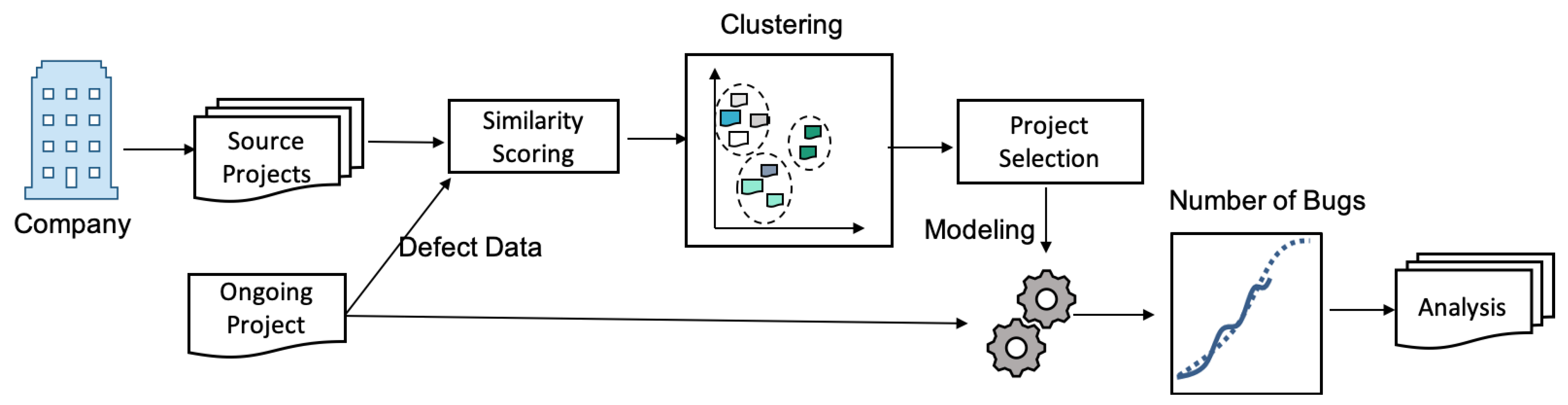
Mathematics 09 02945 g001
Figure 2. Overview of the DC-SRGM model.
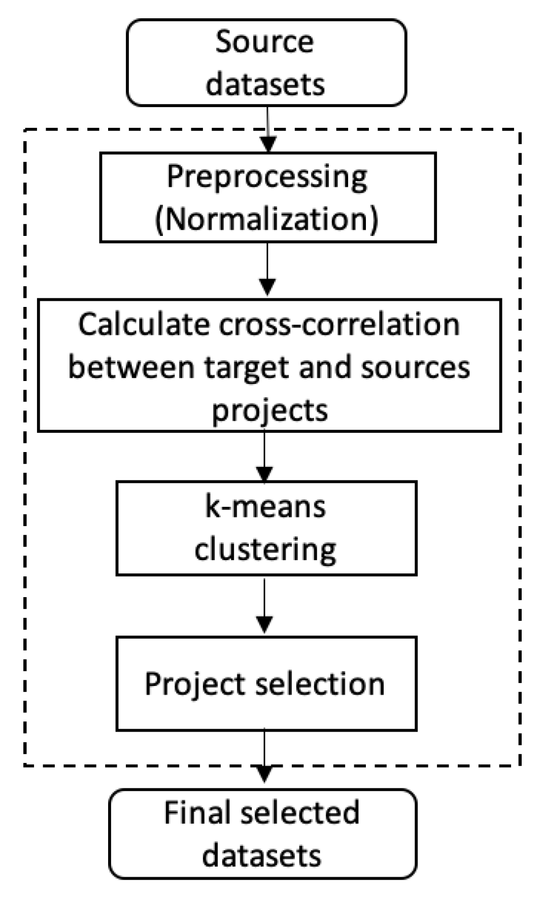
Mathematics 09 02945 g002
Figure 3. Project selection process.
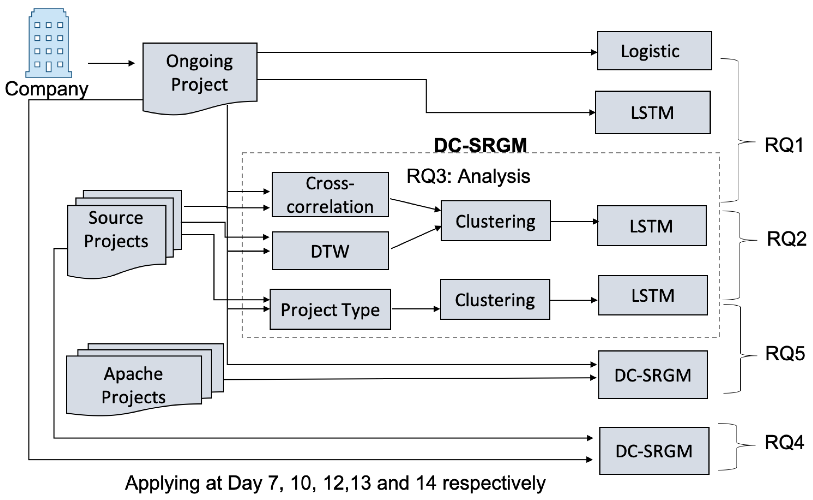
Mathematics 09 02945 g003
Figure 4. Model training process.
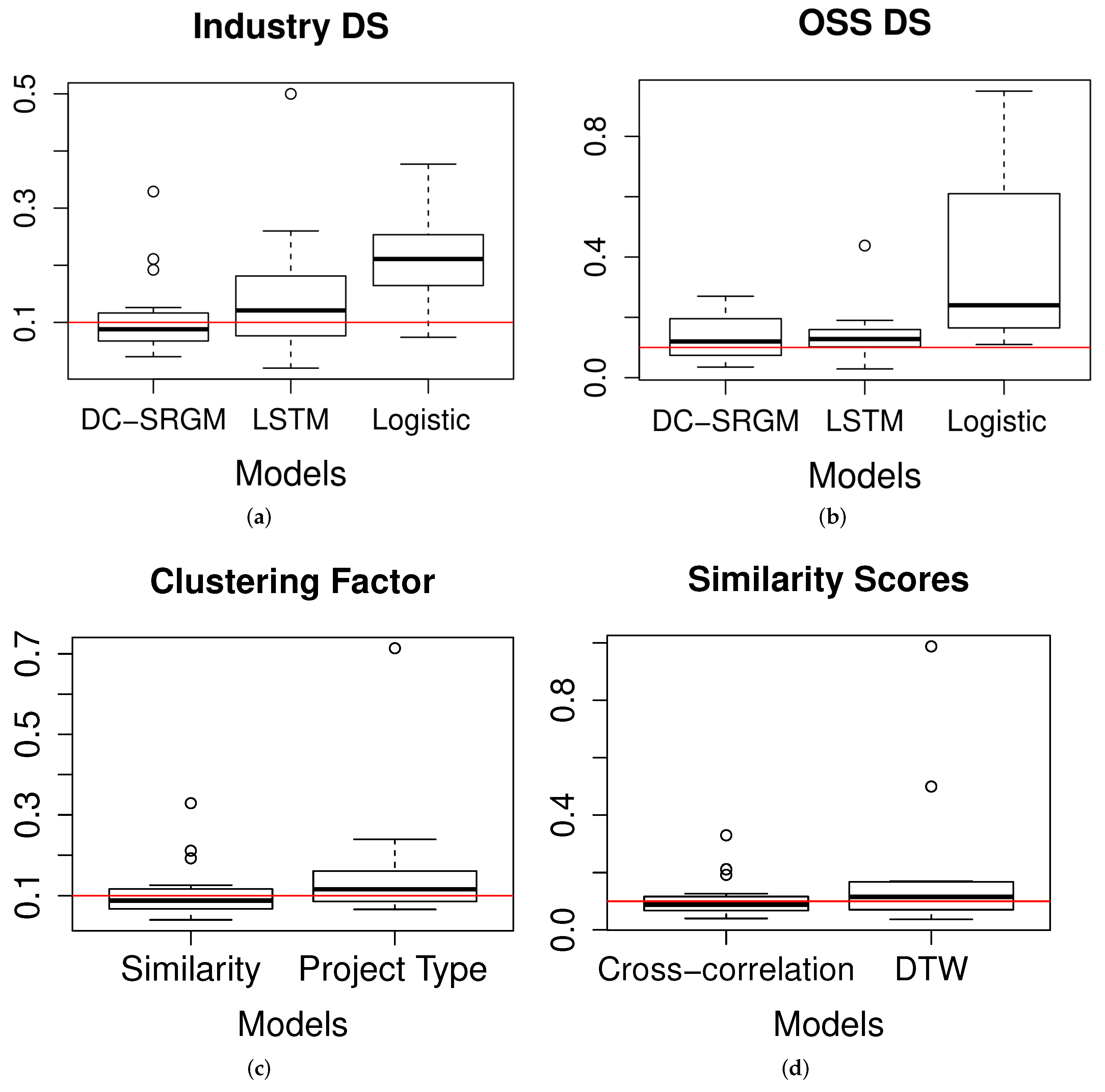
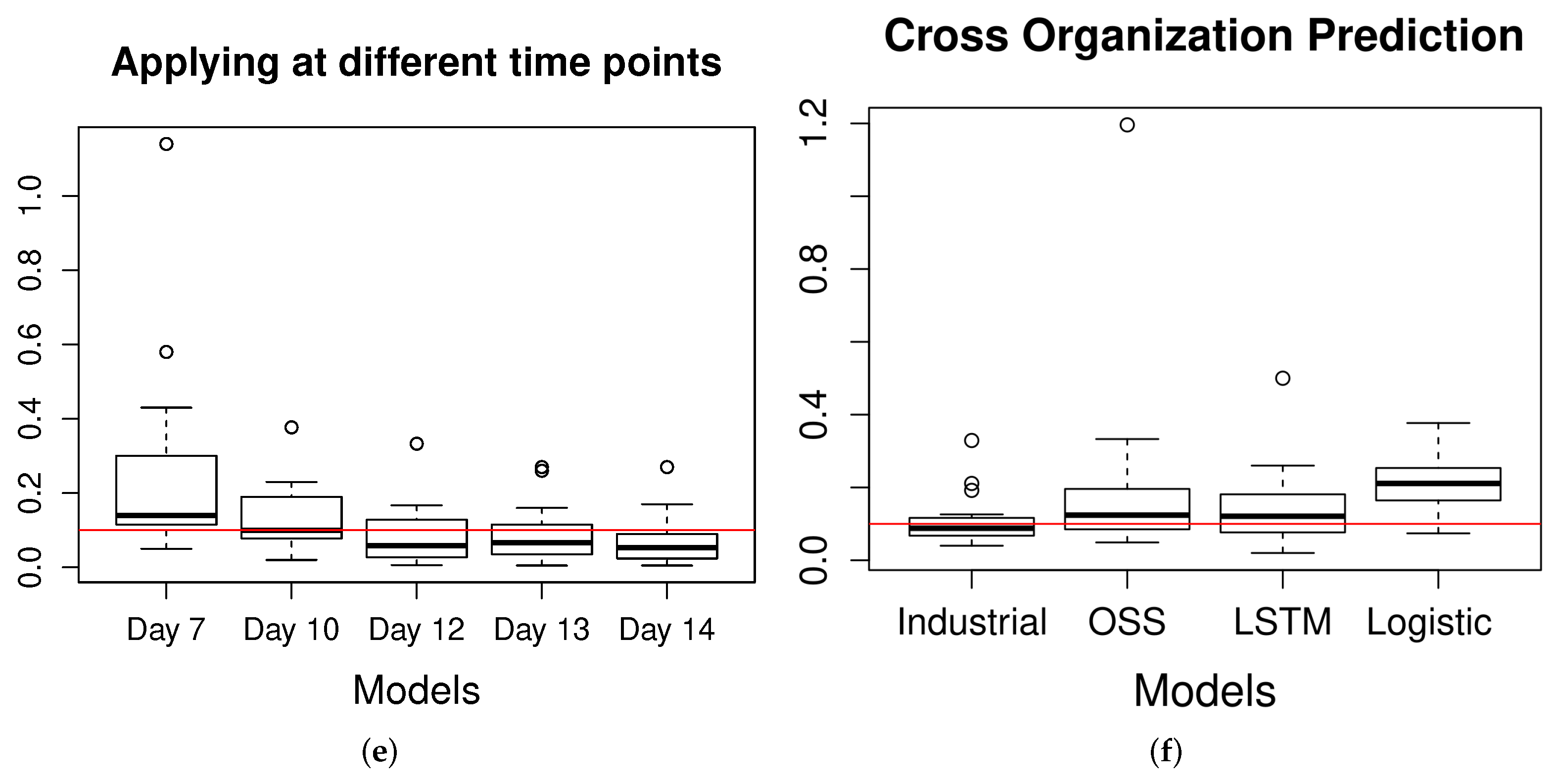
Mathematics 09 02945 g004
Figure 6. Comparison of the model prediction accuracy in terms of average error, AE. (a) Performance in industrial datasets (DS), (b) Performance in OSS datasets, (c) DC-SRGM based on project similarity and project domain type, (d) DC-SRGM based on cross-correlation and DTW, (e) DC-SRGM applied at the different number of days, and (f) DC-SRGM across organizations.
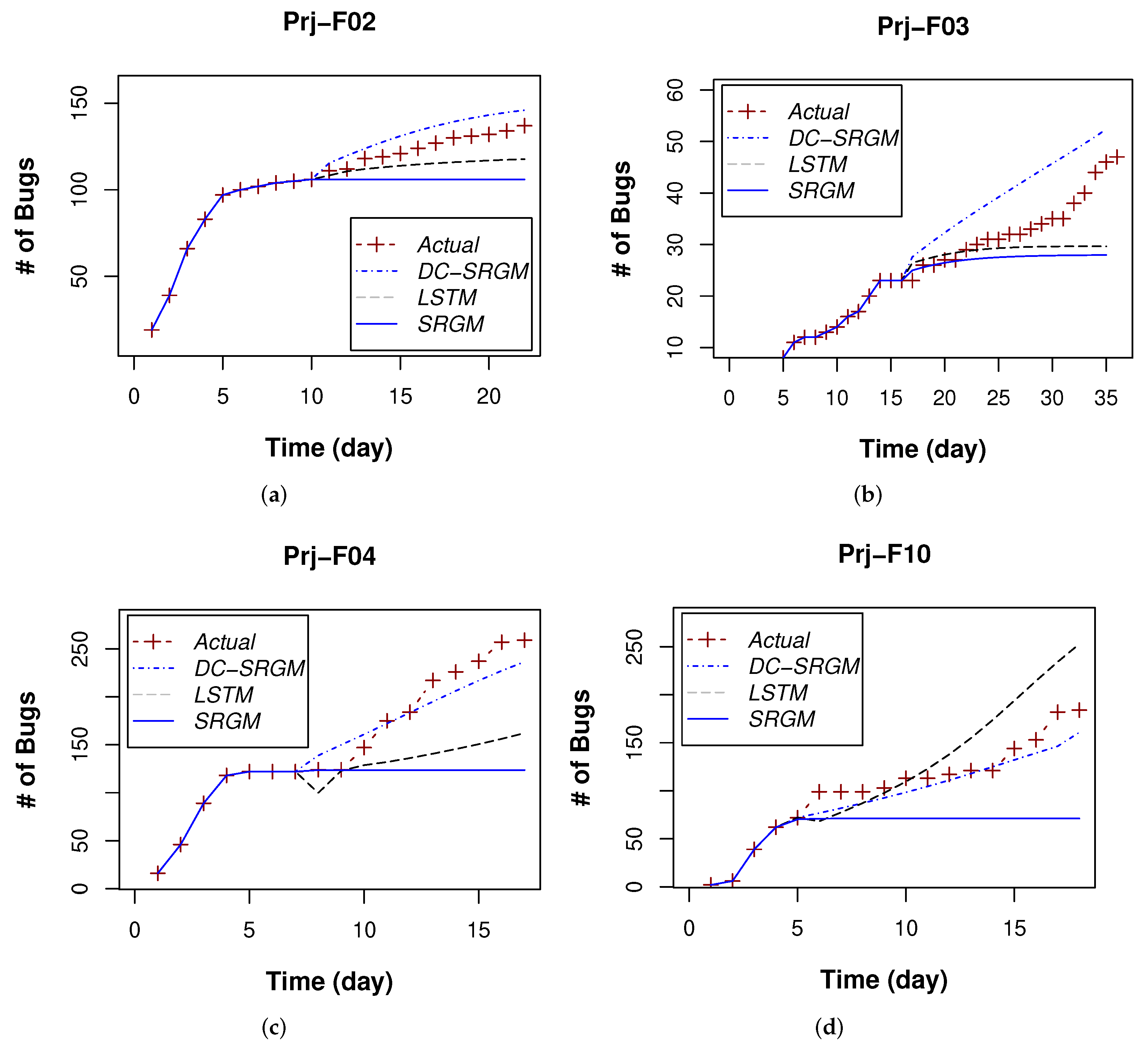
Mathematics 09 02945 g006aMathematics 09 02945 g006b
Figure 7. Predicted number of bugs at the middle of the projects. Actual, DC-SRGM, LSTM, SRGM represent the actual detected number of bugs, the prediction by DC-SRGM, the LSTM model, and the Logistic SRGM model, respectively. (a) Project F02, (b) F03, (c) F04, and (d) F10.
Mathematics 09 02945 g007
Table 1. Industrial project details.
ProjectDays# of Bugs
F011991
F0222137
F031247
F0417259
F0519188
F0626263
F0715146
F081797
F091699
F1018184
F111474
F1225351
F1322187
F1434331
F1518752
Table 2. OSS projects details.
ProjectDays# of BugsStudied Version
Camel36322.15.12.15.2
Ignite481492.52.6
Jclouds175252.1.02.1.1
Karaf56644.14.2
Lucene9166.6.06.6.1
Maven160223.5.13.5.2
Shiro3061.3.01.3.1
Spark991852.3.12.3.2
Syncope80362.0.22.0.3
Tez120270.6.00.6.1
Zookeeper86143.4.123.4.13
Table 3. Summary of the clustering factors.
SimilarityMax BugsMax Days
0∼147∼75214∼36
Table 4. Summary of the clustering results. Projects are generally clustered into three groups according to similarity scores and the project scales. Grad, Expo and Grad, and Expo indicate the growth of the number of bugs is gradually increasing, exponentially increasing and gradually increasing, and exponentially increasing.
ClusterClustered ProjectsMax BugsMax DaysGrowthType
C1F01, F02, F04, F05, F07, F08, F09, F10, F1191∼18814∼22GradSimilarity
C2F12, F15540∼75218∼24Expo# Bugs
C3F03, F06, F13, F1447∼33122∼36Expo and Grad# Days
Table 5. Summary of the clustering results by project. Grad, Expo and Grad, Expo, and Const indicate that the number of bugs is gradually increasing, exponentially increasing and gradually increasing, exponentially increasing, and constantly increasing.
ProjectClusterActual GrowthPrediction Result
F01C1GradGrad
F02C1GradGrad
F03C3GradGrad
F04C1GradGrad
F05C1GradGrad
F06C3ExpoExpo
F07C1Grad and ExpoGrad
F08C2GradGrad
F09C3Expo and GradGrad
F10C4GradGrad
F11C5GradGrad
F12C2ExpoExpo and Grad
F13C3Expo and GradExpo and Grad
F14C3Expo and GradConst
F15C2ExpoExpo
Table 6. Comparison of DC-SRGM with the LSTM and Logistic models by the AE values. Bold denotes the best AE values. W/L is the number of datasets that each method is better and worse than. “# DS Threshold below 0.1” is the number of datasets for which each model’s performance is lower than the threshold.
ProjectDC-SRGMLSTMLogistic
F010.0670.0400.266
F020.0710.0800.146
F030.1920.1300.142
F040.0910.2600.377
F050.0750.1270.218
F060.0400.0900.211
F070.3290.5000.146
F080.0490.1040.187
F090.0550.0480.146
F100.0880.1210.214
F110.0680.0730.074
F120.0950.1610.359
F130.2110.2430.348
F140.1070.0200.183
F150.1260.2010.191
Average0.1100.1460.220
Improved%-+24.6%+50%
W/L10/54/111/14
# DS Threshold below 0.11061
Table 7. Prediction Accuracy of the models on OSS datasets by the AE values. Bold denotes the best AE Values. W/L is the number of datasets for which each method is better and worse than. “# DS Threshold below 0.1” is the number of datasets that each model’s performance is lower than the threshold.
ProjectDC-SRGMLSTMLogistic
Camel0.0810.0990.440
Ignite0.0670.0630.110
Jclouds0.1900.0290.260
Karaf0.0350.1050.830
Lucene0.2700.4380.950
Maven0.1200.1220.240
Shiro0.1000.1390.110
Spark0.2010.1390.190
Syncope0.2400.1280.220
Tez0.0370.1800.780
Zookeeper0.1330.1900.140
Average0.1340.1480.388
Improved%-+9.45%+65.4%
W/L7/44/70/11
# DS Threshold below 0.1531
Table 8. Statistic results with the Nemenyi test for the effectiveness of DC-SRGM. * and ** denote that there were significant differences in the groups as the significance levels were 0.1 and 0.01, respectively.
Modelsp_Value
IndustryDC-SRGM and LSTM0.0710 *
DC-SRGM and Logistic0.0045 **
OSSDC-SRGM and LSTM0.3657
DC-SRGM and Logistic0.0288 *
Table 9. Comparison of the prediction accuracy of DC-SRGM using project similarity and project domain type as clustering factors. W/L is the number of datasets that each method is better and worse than. “# DS Threshold below 0.1” is the number of datasets for which each method’s performance is lower than the threshold.
ProjectProject SimilarityProject Domain Type
F010.0670.074
F020.0710.091
F030.1920.129
F040.0910.137
F050.075
F060.0400.119
F070.3290.714
F080.0490.186
F090.0550.113
F100.0880.096
F110.0680.066
F120.095
F130.2110.239
F140.107
F150.1260.080
Average0.1100.170
W/L9/33/9
# DS Threshold below 0.1107
Table 10. Comparison of the prediction accuracy DC-SRGM using cross-correlation and DTW as similarity measures. W/L is the number of datasets that each method is better and worse than. “# DS Threshold below 0.1” is the number of datasets for which each method’s performance is lower than the threshold.
ProjectCross-CorrelationDTW
F010.0670.037
F020.0710.039
F030.1920.499
F040.0910.081
F050.0750.048
F060.0400.170
F070.3290.988
F080.0490.166
F090.0550.089
F100.0880.115
F110.0680.169
F120.0950.115
F130.2110.165
F140.1070.060
F150.1260.089
Average0.1100.188
W/L8/77/8
# DS Threshold below 0.1107
Table 11. Comparison of DC-SRGM for different numbers of days. “# DS Threshold below 0.1” is the number of datasets for which each model’s performance is lower than the threshold.
ProjectDay 7Day 10Day 12Day 13Day 14
F010.0700.0780.0720.0600.060
F020.0500.0300.0450.0400.050
F030.5800.3770.1670.1600.170
F040.1000.0870.0730.0310.028
F050.1300.0700.0290.0240.020
F060.1400.2250.0390.0430.030
F071.1400.7800.3330.2700.140
F080.4100.0980.0090.0110.015
F090.1600.1110.0070.0050.005
F100.1900.1120.1430.1100.079
F110.1400.0200.0060.0070.007
F120.1900.2300.0580.0660.060
F130.4300.1900.0250.2600.270
F140.1300.1000.1310.1200.100
F150.0800.1900.1250.0870.050
Average0.2620.1790.0900.0920.072
# DS Threshold below 0.14/157/1510/1510/1512/15
Table 12. Accuracies of DC-SRGM built with industrial datasets and cross-organization datasets (OSS) are compared with the LSTM model and Logistic model. W/L is the number of datasets that each method is better and worse than. “Threshold below 0.1” is the number of datasets for which each method’s performance is lower than the threshold.
ProjectDC-SRGMLSTMLogistic
Industry DSCross-org DS
F010.0670.0510.0400.266
F020.0710.1040.0800.146
F030.1920.1070.1300.142
F040.0910.1240.2600.377
F050.0750.0490.1270.218
F060.0400.1360.0900.211
F070.3290.1960.5000.146
F080.0490.3330.1040.187
F090.0550.1960.0480.146
F100.0880.1200.1210.214
F110.0680.0660.0730.074
F120.0950.0660.1610.359
F130.2110.2050.2430.348
F140.1070.1720.0200.183
F150.1260.1960.2010.191
Average0.1100.1410.1460.220
W/L6/96/92/131/14
# DS Threshold below 0.110461
Publisher’s Note: MDPI stays neutral with regard to jurisdictional claims in published maps and institutional affiliations.

