Nonlinearly Preconditioned FETI Solver for Substructured Formulations of Nonlinear Problems

Abstract

We consider the finite element approximation of the solution to elliptic partial differential equations such as the ones encountered in (quasi)-static mechanics, in transient mechanics with implicit time integration, or in thermal diffusion. We propose a new nonlinear version of preconditioning, dedicated to nonlinear substructured and condensed formulations with dual approach, i.e., nonlinear analogues to the Finite Element Tearing and Interconnecting (FETI) solver. By increasing the importance of local nonlinear operations, this new technique reduces communications between processors throughout the parallel solving process. Moreover, the tangent systems produced at each step still have the exact shape of classically preconditioned linear FETI problems, which makes the tractability of the implementation barely modified. The efficiency of this new preconditioner is illustrated on two academic test cases, namely a water diffusion problem and a nonlinear thermal behavior.

1. Introduction

We consider the finite element approximation of the solution to elliptic partial differential equations such as the ones encountered in (quasi)-static mechanics, in transient mechanics with implicit time integration, or in thermal diffusion. Space domain decomposition methods offer an interesting framework for the distribution of the resolution.

In addition, in the linear(ized) case, they provide powerful preconditioners for an efficient iteration solution. Among the most famous, let us cite in the case of overlapping decompositions, the (Restricted) Additive Schwarz methods (RAS/AS) [1,2] and, in the absence of overlap, the Finite Element Tearing and Interconnecting (FETI) [3] and the Balancing Domain Decomposition (BDD) [4].

These methods have in common to associate (approximations of) local inverse operators and a coarse propagator for long range effects (associated with the Saint-Venant principle in mechanics). The coarse propagator can be of additive form or implemented as a projector. It can also be replaced by a set of well chosen continuity conditions, like in the FETI-DP [5] or BDDC [6] methods. Note that the local inverses can also be replaced by well chosen (generalized) Robin conditions in the Optimized Schwarz (OSM) [7]/FETI—2 Lagrange Multipliers (FETI2LM) [8] methods.

It is now well understood that the decomposition can trigger numerical difficulties which might impair the scalability of the methods. In order to compensate the loss of scalability, the coarse problem can be enriched by well-chosen constraints—built through localized generalized eigenvalue problems [9,10,11,12], or the classical preconditioner can be replaced by a multipreconditioner [13,14].

When carefully implemented, these methods reach very interesting parallel speed-ups on a large class of problems, for a wide range of processors. Anyhow, each iteration of the distributed Krylov solver involves all-neighbor exchanges and all-to-all reductions. All-neighbor exchanges scale well because the number of neighbors can not become excessive. All-to-all reductions, even if they can be gathered and hidden [15], may lead to loss of performance. It is then of importance to propose methods that reduce the number of communications even at the cost of increased local computations.

In the context of nonlinear problems, the classical approach is to use a Newton solver in an outer loop [16,17]. The decomposition of the domain then enables to distribute the computation of the residual and of the tangent operator. Usually, an inexact Newton strategy is adopted in order to limit the number of Krylov iterations involved in the solution to the tangent system (computed by the chosen DDM solver) [18]. The initials for the classical approach are NKS for Newton–Krylov–Schur (or Schwarz depending on the chosen DD preconditioner).

Starting from the observation that NKS methods do not take advantage of the domain decomposition to deal with the nonlinearity, a new class of iterative nonlinear solvers has been developed: they allow independent nonlinear computations per subdomains, with the hope that the number of exchanges would be reduced and energy could be saved [19].

In the frame of Schwarz methods, we can cite the one- or two-level Additive Scharwz Preconditioned by Inexact Newton (ASPIN) [20,21] or Restricted Additive Scharwz Preconditioned by Exact Newton (RASPEN) [22,23] solvers, or the Large Time Increment (LATIN) method [24] and the global/local non-invasive coupling [25] which are very close to Optimized Schwarz methods. In the frame of non-overlapping methods, the solvers sometime took the name of “nonlinear relocalization techniques”. Nonlinear counterparts to classical non-overlapping DD methods were considered, see [26] for a global framework of the primal (BDD)/dual (FETI)/mixed (FETI2LM) approaches, and [27] for an improved impedance in the mixed approach. Nonlinear FETI-DP and BDDC were proposed in [28] (see also [29] for BDDC), and improved and assessed at a large scale in [30,31].

The non-overlapping nonlinear methods (which will be named with the -NL suffix) can be formalized by the introduction of nonlinear primal/dual/mixed Stecklov-Poincaré operators per subdomain (for instance the primal Stecklov–Poincaré operator is the discrete Dirichlet-to-Neumann operator associated with the nonlinear Dirichlet solve on the subdomain). The global nonlinear problem is formally condensed into a nonlinear interface problem.

Note that because of the vastness of nonlinear problems, it is hard to derive general convergence results. The validity of the methods is limited to certain classes of problems. The reader may refer to [32] for a review of nonlinear problems where stable solutions can be found and where nonlinear Stecklov-Poincaré operators can thus be defined. In general the best property obtainable is the local convergence around a stable unique solution.

When applying a Newton solver on the condensed problem, one alternates local independent nonlinear solves with given boundary conditions, and interface corrections obtained by solving the tangent condensed system. This system has exactly the structure of a linear DDM problem and can be solved by the classical linear Krylov solvers preconditioned by DDM mentioned above.

The hope when using these methods is that letting the subdomains undergo independent nonlinear evolution provides a better estimation of the state of the structure which should limit the number of outer Newton iterations and the communications associated with the global tangent solver. Furthermore, these methods try to avoid useless computations on subdomains associated with linear evolutions which have no influence on the global convergence, allowing the CPUs to idle and reduce their energy consumption.

In this paper, our objective is to double the intensity of the local independent nonlinear computations by modifying the condensed problem to be solved. The method can be interpreted as proposing a nonlinear preconditioner [33] to the nonlinear condensation approaches. Even if the idea could be ported to any BDD(C)-NL, or FETI(DP)-NL method, it will appear that under the chosen hypothesis (equivalent to infinitesimal strain in mechanics), the FETI-NL method leads to a much simpler problem to be solved since the unknown is sought in a vector space instead of a manifold.

When applying a Newton algorithm to this nonlinear preconditioned condensed system, one alternates a sequence of two independent nonlinear local solves (one Neumann problem and one Dirichlet problem separated by one all-neighbor communication) and an interface tangent solve which has the structure of a linear preconditioned FETI problem. Hopefully the sequence of two local nonlinear solves will reduce the need of global Newton iterations and thus the number of calls to the communication-demanding Krylov solver.

The paper is organized as follows: in Section 2, the principle of nonlinear substructuring and condensation is recalled with emphases on the FETI-NL method. In Section 3 the nonlinear preconditioning for the FETI-NL method is exposed. Limited academic assessments are given in Section 4 related to a water diffusion in soils problem, and a nonlinear thermal evolution. Section 5 concludes the paper.

2. Nonlinear Substructuring and Condensation

2.1. Reference Problem, Notations

2.1.1. Global Nonlinear Problem

We consider a nonlinear partial differential equation on a domain $\mathsf{\Omega }$, representative of a quasi-static structural mechanical or thermal problem for instance, satisfied by the unknown u (displacement, temperature...). Dirichlet conditions are imposed on a part ${\partial }_u\mathsf{\Omega }\ne \varnothing$ of the boundary, and Neumann conditions on the complementary part ${\partial }_f\mathsf{\Omega }$. After discretization with the Finite Element method (typically using $H^1$ conforming element), the problem to be solved can be written as:

$$g_{int}\left(u\right)+g_{ext}=0.$$

(1)

The vector of external forces $g_{ext}$ takes into account boundary conditions (Dirichlet or Neumann) and dead loads, the operator of internal forces $g_{int}$ refers to the discretization of the homogeneous partial differential equation. Note that such a problem may also represent the study at a given time step of a transient problem with implicit time integration. We assume that $g_{int}$ is differentiable and such that the tangent matrices are symmetric positive semi-definite (the semi-definiteness being typically due to the existence of rigid body motions). We also assume the well-posedness of the problem (it possesses a unique, stable, solution), and that a classical Newton–Raphson strategy could be deployed to find it.

Remark 1.

In linear elasticity, under the small perturbations hypothesis, one has:

$$g_{int}\left(u\right)=-Ku,$$

with K the stiffness matrix of the structure.

2.1.2. Substructuring and Local Equilibriums

The global domain $\mathsf{\Omega }$ is partitioned into $N_s$ subdomains $\left({\mathsf{\Omega }}^{\left(s\right)}\right)$, corresponding to the decomposition of the nonlinear problem (1) into $N_s$ nonlinear subproblems:

$$g_{int}^{\left(s\right)}\left(u^{\left(s\right)}\right)+g_{ext}^{\left(s\right)}+T^{{\left(s\right)}^T}{\lambda }_b^{\left(s\right)}=0,$$

(2)

where ${\lambda }_b^{\left(s\right)}$ is the unknown local nodal reaction, introduced to represent interactions of subdomain ${\mathsf{\Omega }}^{\left(s\right)}$ with neighboring subdomains: ${\lambda }_b^{\left(s\right)}$ is defined on the “boundary” with neighbors (index b, to be opposed to internal degrees of freedom, index i) and $T^{{\left(s\right)}^T}$ is the extension-by-zero operator (transpose of the trace operator).

Equation (2) will be referred to as “local equilibrium”. For a given boundary condition, all the fields involved in (2) can be computed. In the following, we consider two types of boundary conditions to be imposed on the interface between subdomains: primal (Dirichlet) conditions or dual (Neumann) conditions. All formula are detailed in [26].

Primal Approach

We assume the well-posedness of local Dirichlet problems, so that we can define on subdomain ${\mathsf{\Omega }}^{\left(s\right)}$ the nonlinear primal analogue $s_{nl}^{\left(s\right)}$ to the primal Steklov-Poincaré operator [34] (i.e., a discrete Dirichlet-to-Neumann operator). The interface nodal reaction $\left({\lambda }_b^{\left(s\right)}\right)$ resulting from the local equilibrium (2) is then defined uniquely, and it can be expressed as a function of the given boundary displacement $u_b^{\left(s\right)}$ and external forces $g_{ext}^{\left(s\right)}$:

$${\lambda }_b^{\left(s\right)}=s_{nl}^{\left(s\right)}\left(u_b^{\left(s\right)};g_{ext}^{\left(s\right)}\right).$$

(3)

Property 1.

The tangent operator $S_t^{\left(s\right)}$ to $s_{nl}^{\left(s\right)}$ can be explicitly computed as a function of the tangent stiffness matrix $K_t^{\left(s\right)}$:

$$\begin{array}{c}\hfill \forall s\in \left\{0,\dots ,N_s\right\},S_t^{\left(s\right)}=\frac{\partial s_{nl}^{\left(s\right)}}{\partial u_b^{\left(s\right)}}=K_{t_{bb}}^{\left(s\right)}-K_{t_{bi}}^{\left(s\right)}{K}_{t_{ii}}^{{\left(s\right)}^{-1}}{K}_{t_{ib}}^{\left(s\right)}.\end{array}$$

(4)

Moreover, in the linear case, the discrete Dirichlet-to-Neumann operator, written $s_l^{\left(s\right)}$, is affine, with the constant term being associated with external forces:

$$\begin{array}{cc}\hfill & s_l^{\left(s\right)}\left(u_b^{\left(s\right)};g^{\left(s\right)}\right)=S_t^{\left(s\right)}{u}_b^{\left(s\right)}-b_p^{\left(s\right)},\hfill \\ \hfill \mathit{with}& b_p^{\left(s\right)}=g_b^{\left(s\right)}-K_{t_{bi}}^{\left(s\right)}{K}_{t_{bi}}^{s^{-1}}{g}_i^{\left(s\right)}.\hfill \end{array}$$

(5)

Dual Approach

We consider Neumann conditions on the interface of subdomains. In the following we make an assumption equivalent to the infinitesimal strain hypothesis in mechanics: for any subdomain ${\mathsf{\Omega }}^{\left(s\right)}$ lacking Dirichlet conditions (aka floating subdomain), there exists a basis $R^{\left(s\right)}$ of rigid body motions which satisfies:

$$\forall u^{\left(s\right)},\left\{\begin{array}{cc}\hfill & g_{int}^{\left(s\right)}(u^{\left(s\right)}+R^{\left(s\right)}{\alpha }^{\left(s\right)})=g_{int}^{\left(s\right)}\left(u^{\left(s\right)}\right),\forall {\alpha }^{\left(s\right)}\hfill \\ \hfill & R^{{\left(s\right)}^T}{g}_{int}^{\left(s\right)}\left(u^{\left(s\right)}\right)=0\hfill \end{array}\right..$$

(6)

The basis of rigid body motions is directly linked to the kernel of the tangent matrix:

$$R^{\left(s\right)}=Ker\left(K_t^{\left(s\right)}\right),\mathrm{with}{K}_t^{\left(s\right)}=\frac{\partial g_{int}^{\left(s\right)}}{\partial u^{\left(s\right)}}.$$

Let $r^{\left(s\right)}$ denote the number of rigid body motions of subdomain ${\mathsf{\Omega }}^{\left(s\right)}$, that is to say the number of columns of $R^{\left(s\right)}$.

Remark 2.

Mechanically speaking, the above hypothesis excludes problems with large displacements, and leads us to focus on material nonlinearity.

Hypothesis (6) applied to the local equilibrium (2) leads to the following compatibility condition:

$$R^{{\left(s\right)}^T}\left(g_{ext}^{\left(s\right)}+T^{{\left(s\right)}^T}{\lambda }_b^{\left(s\right)}\right)=0.$$

(7)

Under this condition on ${\lambda }_b^{\left(s\right)}$, and assuming the global problem is well posed, we can assume, at least locally the existence of a nonlinear dual analogue $f_{nl}^{\left(s\right)}$ to the dual Steklov-Poincaré operator [34] (i.e., a discrete Neumann-to-Dirichlet operator). The solution $u^{\left(s\right)}$ of each local equilibrium is then defined uniquely, up to a rigid body mode $R^{\left(s\right)}{\alpha }^{\left(s\right)}$, and interface local unknowns can be expressed as:

$$u_b^{\left(s\right)}=f_{nl}\left({\lambda }_b^{\left(s\right)};g^{\left(s\right)}\right)+T^{\left(s\right)}{R}^{\left(s\right)}{\alpha }^{\left(s\right)}.$$

(8)

Property 2.

The tangent operator $F_t^{\left(s\right)}$ to $f_{nl}^{\left(s\right)}$ can be explicitly computed as a function of a pseudo-inverse of the tangent stiffness $K_t^{\left(s\right)}$ [26]:

$$\begin{array}{c}\hfill F_t^{\left(s\right)}=\frac{\partial f_{nl}^{\left(s\right)}}{\partial {\lambda }_b^{\left(s\right)}}=T^{\left(s\right)}{K}_t^{{\left(s\right)}^{†}}{T}^{{\left(s\right)}^T}.\end{array}$$

(9)

Moreover, in the linear case, the Neumann-to-Dirichlet operator – written $f_l^{\left(s\right)}$ – is affine, with the constant term associated with external forces:

$$\begin{array}{cc}\hfill & F_l^{\left(s\right)}\left({\lambda }_b^{\left(s\right)};g^{\left(s\right)}\right)=F_t^{\left(s\right)}{\lambda }_b^{\left(s\right)}+b_d^{\left(s\right)},\hfill \\ \hfill \mathit{with}& b_d^{\left(s\right)}=T^{\left(s\right)}{K}_t^{{\left(s\right)}^{†}}{g}^{\left(s\right)}.\hfill \end{array}$$

(10)

Note the link between the primal and dual right-hand sides in the linear case: $b_d^{\left(s\right)}=F_t^{\left(s\right)}{b}_p^{\left(s\right)}$.

2.2. Assembly Operators and Block Notations

Let ${\Gamma }^{\left(s\right)}$ denote the set of interface degrees of freedom of Subdomain ${\mathsf{\Omega }}^{\left(s\right)}$. The Global primal interface is written ${\Gamma }_A={\cup }_s{\Gamma }^{\left(s\right)}$. Primal assembly operators $A^{\left(s\right)}$ are defined as canonical prolongation operators from ${\Gamma }^{\left(s\right)}$ to ${\Gamma }_A$: $A^{\left(s\right)}$ is a full-ranked boolean matrix of size $n_A\times n_b^{\left(s\right)}$ - where $n_A$ is the size of global primal interface ${\Gamma }_A$ and $n_b^{\left(s\right)}$ the number of interface degrees of freedom of subdomain ${\mathsf{\Omega }}^{\left(s\right)}$.

We use block notations to handle simultaneously quantities defined on subdomains. Local vectors are concatenated by rows, assembly operators are concatenated by columns, local matrices are concatenated diagonally:

$$\begin{array}{cc}\hfill & \mathrm{vector}:\mathbf{x},\mathrm{matrix}:\mathbf{M},\mathrm{assembly}:\mathbf{A},\mathbf{B}\hfill \\ \hfill & \mathbf{x}=\left(\begin{array}{c}{x}^{\left(1\right)}\\ ⋮\\ x^{\left(N_s\right)}\end{array}\right),\mathrm{matrix}:\mathbf{M}=\left(\begin{array}{ccc}{M}^{\left(1\right)}& 0& 0\\ 0& \ddots & 0\\ 0& 0& M^{\left(N_s\right)}\end{array}\right),\begin{array}{cc}\hfill & \mathbf{A}=\left(\begin{array}{c}{A}^{\left(1\right)},\dots ,A^{\left(N_s\right)}\end{array}\right),\hfill \\ \hfill & \mathbf{B}=\left(\begin{array}{c}{B}^{\left(1\right)},\dots ,B^{\left(N_s\right)}\end{array}\right).\hfill \end{array}\hfill \end{array}$$

(11)

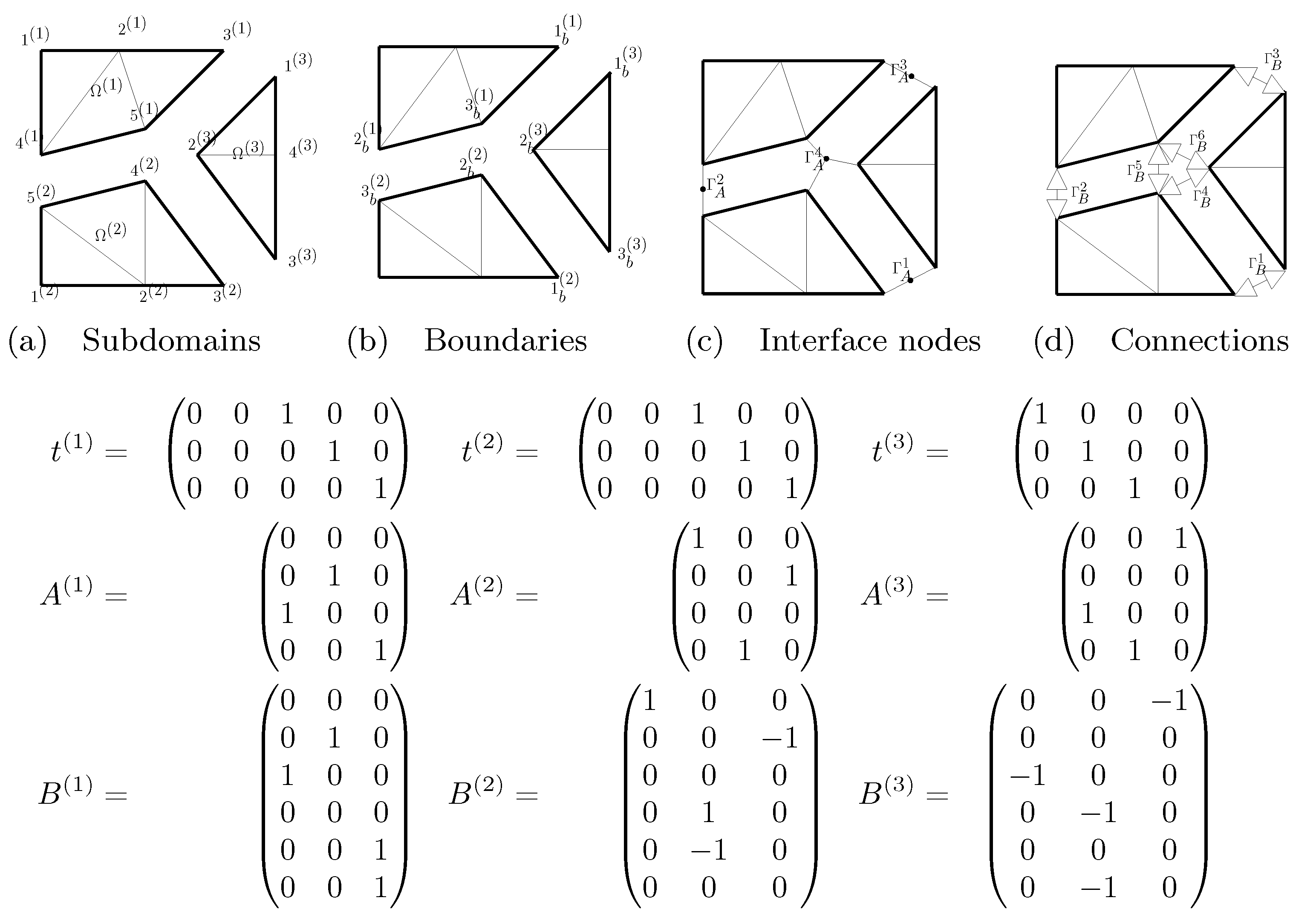
Any matrix $\mathbf{B}$ satisfying $Range\left(\mathbf{B}\right)=Ker\left(\mathbf{A}\right)$ can be assigned to dual assembly operator—see Figure 1 for the most classical choice. Note that in this case, multiple-points lead to $\mathbf{B}$ being rank-deficient. The number of relations characterizing the global dual interface ${\Gamma }_B$ is written $n_B$.

We introduce the classical primal and dual scaled assembly operators $\tilde{\mathbf{A}}$ and $\tilde{\mathbf{B}}$ [35], they satisfy the following properties:

$$\begin{array}{cc}\hfill & \mathbf{A}{\tilde{\mathbf{A}}}^T=\tilde{\mathbf{A}}{\mathbf{A}}^T=\mathbf{I},\hfill \\ \hfill & \mathbf{B}{\tilde{\mathbf{B}}}^T\mathbf{B}=\mathbf{B},\tilde{\mathbf{B}}{\mathbf{B}}^T\tilde{\mathbf{B}}=\tilde{\mathbf{B}}.\hfill \end{array}$$

(12)

Classically, the scaling operators are built as follows:

$$\left\{\begin{array}{cc}\hfill & \tilde{\mathbf{A}}={\left(\mathbf{A}\mathbf{D}{\mathbf{A}}^T\right)}^{-1}\mathbf{A}\mathbf{D},\hfill \\ \hfill & \tilde{\mathbf{B}}={\left(\mathbf{B}{\mathbf{D}}^{-1}{\mathbf{B}}^T\right)}^{†}\mathbf{B}{\mathbf{D}}^{-1},\hfill \end{array}\right.\mathrm{with}{D}^{\left(s\right)}=I^{\left(s\right)}\mathrm{or}diag\left(K_{t_{bb}}^{\left(s\right)}\right).$$

(13)

Note that if the same matrix $\mathbf{D}$ is chosen in definition of the primal and dual scaled assembly operators then the following property holds [36]:

$${\mathbf{A}}^T\tilde{\mathbf{A}}+{\tilde{\mathbf{B}}}^T\mathbf{B}=\mathbf{I}.$$

(14)

Remark 3.

The following trivial properties are worth recalling:

$$\mathrm{Range}\left(\mathbf{B}\right)\cap \mathrm{Ker}\left({\mathbf{B}}^T\right)=\left\{0\right\} \mathit{and} \mathrm{Range}\left(\tilde{\mathbf{B}}\right)\cap \mathrm{Ker}\left({\mathbf{B}}^T\right)=\left\{0\right\}.$$

2.3. Interface Problem and Solving Strategy

The problem to be solved is the concatenation of all local equilibriums:

$${\mathbf{g}}_{\mathbf{int}}\left(\mathbf{u}\right)+{\mathbf{g}}_{\mathbf{ext}}+{\mathbf{T}}^T{\lambda }_{\mathbf{b}}=0.$$

(15)

completed by the classical transmission conditions—continuity of displacements and balance of reactions:

$$\left\{\begin{array}{c}\hfill \mathbf{B}{\mathbf{u}}_{\mathbf{b}}=0,\\ \hfill \mathbf{A}{\lambda }_{\mathbf{b}}=0.\end{array}\right.$$

(16)

This section recalls the principle of nonlinear substructuring and condensation for dual and primal approach. More details can be found in [26].

2.3.1. Dual Approach

Formulation of the Condensed Problem

The dual formulation consists of using the interface traction ${\lambda }_B$, defined on ${\Gamma }_B$, as main unknown. Local reactions are defined as ${\lambda }_{\mathbf{b}}={\mathbf{B}}^T{\lambda }_B$ and thus they are automatically balanced $(\mathbf{A}{\lambda }_{\mathbf{b}}=0)$. The local equilibrium is used in its dual form (8) in order to define displacements whose gap measures the convergence of the solver. Using admissibility condition (7), and writing $r=\sum r^{\left(s\right)}$ the total number of rigid body motions, the system to be solved reads:

$$\begin{array}{cc}\hfill & \mathrm{Find}{\lambda }_B\in {\mathbb{R}}^{n_B},\alpha \in {\mathbb{R}}^r\mathrm{such}\mathrm{that}:\hfill \\ \hfill & \mathbf{B}({\mathbf{f}}_{\mathbf{nl}}({\mathbf{B}}^T{\mathbf{\lambda }}_B;{\mathbf{g}}_{\mathbf{ext}}) + \mathbf{TR}\alpha ) =0,\hfill \end{array}$$

(17)

$${\mathbf{R}}^T\left({\mathbf{g}}_{\mathbf{ext}}+{\mathbf{T}}^T{\mathbf{B}}^T{\lambda }_{B_0}\right)=0,$$

(18)

We introduce the notations ${\mathbf{R}}_{\mathbf{b}}=\mathbf{T}\mathbf{R}$ and ${\mathbf{G}}_B=\mathbf{B}{\mathbf{R}}_{\mathbf{b}}$.

Admissibility Condition: Projection Strategy

In practice, the solution ${\lambda }_B$ to the dual interface condensed problem (17) is sought iteratively in the admissible affine space defined by (18). As in classical linear FETI method, we compute a proper initialization ${\lambda }_{B_0}$ and look for the remaining part in $Ker\left({\mathbf{G}}_B^T\right)$ using the projector ${\mathbf{P}}_B$. The unknown thus takes the following form:

$${\lambda }_B={\lambda }_{B_0}+{\mathbf{P}}_B{\tilde{\lambda }}_B\mathrm{with}:\begin{array}{cc}\hfill & \left\{\begin{array}{cc}& {\mathbf{R}}^T\left({\mathbf{g}}_{\mathbf{ext}}+{\mathbf{T}}^T{\mathbf{B}}^T{\lambda }_{B_0}\right)=0,\hfill \\ \hfill & {\mathbf{R}}_{\mathbf{b}}^T{\mathbf{B}}^T{\mathbf{P}}_B=0.\hfill \end{array}\right.\hfill \end{array}$$

In practice, we use the following expressions:

$$\left\{\begin{array}{cc}\hfill & {\mathbf{P}}_B=\mathbf{I}-{\mathbf{Q}}_B{\mathbf{G}}_B{\left({\mathbf{G}}_B^T{\mathbf{Q}}_B{\mathbf{G}}_B\right)}^{-1}{\mathbf{G}}_B^T,\hfill \\ \hfill & {\lambda }_{B_0}=-{\mathbf{Q}}_B{\mathbf{G}}_B{\left({\mathbf{G}}_B^T{\mathbf{Q}}_B{\mathbf{G}}_B\right)}^{-1}{\mathbf{R}}^T{\mathbf{g}}_{\mathbf{ext}}.\hfill \end{array}\right.$$

(19)

where ${\mathbf{Q}}_B=\tilde{\mathbf{B}}\mathbf{Q}{\tilde{\mathbf{B}}}^T$ is a SPD matrix homogeneous to the (linearized) preconditioner or any of its approximations ($\mathbf{Q}$ is homogeneous to a boundary stiffness matrix). It is crucial to note that the matrix ${\mathbf{Q}}_B$ does not need to be updated during the nonlinear resolution (usually it is at most updated at the beginning of the increments of the Newton solver, ${\mathbf{Q}}_B=\mathbf{I}$ is even a classical choice).

For any ${\tilde{\lambda }}_B$ (even inexact), the magnitude $\alpha$ of the rigid body motions can be computed by minimizing the ${\mathbf{Q}}_B$-norm of the nonlinear interface condensed dual residual, which leads to:

$$\alpha ={\left({\mathbf{G}}_B^T{\mathbf{Q}}_B{\mathbf{G}}_B\right)}^{-1}{\mathbf{G}}_B^T{\mathbf{Q}}_B\mathbf{B}{\mathbf{f}}_{\mathbf{nl}}\left({\mathbf{B}}^T({\lambda }_{B_0}+{\mathbf{P}}_B{\tilde{\lambda }}_B);{\mathbf{g}}_{\mathbf{ext}}\right).$$

(20)

Using this expression for $\alpha$ in Equation (21), one recognizes the transposed projector. Finally the system to be solved can be written as:

$$\mathrm{Find}{\tilde{\lambda }}_B\in {\mathbb{R}}^{n_B}\mathrm{such}\mathrm{that}:{\rho }_B\left({\tilde{\lambda }}_B\right)\equiv {\mathbf{P}}_B^T\mathbf{B}{\mathbf{f}}_{\mathbf{nl}}\left({\mathbf{B}}^T({\lambda }_{B_0}+{\mathbf{P}}_B{\tilde{\lambda }}_B);{\mathbf{g}}_{\mathbf{ext}}\right)=0.$$

(21)

A Newton–Krylov Algorithm

The nonlinear substructuring and condensation method consists of solving interface problem (21) instead of global problem (1). The Newton method applied to this equation leads to, for $k⩾0$:

$$\left\{\begin{array}{cc}\hfill & \mathrm{Solve}\mathrm{for}d{\tilde{\lambda }}_B:\left[\frac{\partial {\rho }_B}{\partial {\tilde{\lambda }}_B}\left({\tilde{\lambda }}_{B_k}\right)\right]d{\tilde{\lambda }}_B=-{\rho }_B\left({\tilde{\lambda }}_{B_k}\right),\hfill \\ \hfill & \mathrm{Update}{\tilde{\lambda }}_{B_{k+1}}={\tilde{\lambda }}_{B_k}+d{\tilde{\lambda }}_B.\hfill \end{array}\right.$$

(22)

Two steps are involved in the solving process:

(i)

Computation of the right-hand side ${\rho }_B\left({\tilde{\lambda }}_{B_k}\right)$ of (22): independent solutions to nonlinear Neumann problems (8) per subdomains. These are computed by applying local Newton algorithms, and the resulting displacement are assembled to build the nonlinear projected interface residual ${\rho }_B\left({\tilde{\lambda }}_{B_k}\right)$.

(ii)

Solution to the tangent system of (22). This tangent system is defined on the interface and it has exactly the structure of a FETI system:

$$\frac{\partial {\rho }_B}{\partial {\tilde{\lambda }}_B}\left({\tilde{\lambda }}_{B_k}\right)={\mathbf{P}}_B^T\mathbf{B}{\mathbf{F}}_{\mathbf{t}}k{\mathbf{B}}^T{\mathbf{P}}_B,$$

where ${\mathbf{F}}_{\mathbf{t}}k$ is the notation for the tangent operator at ${\lambda }_{B_k}$ which is connected to the tangent stiffness matrix (9).

In the following, this solving process will be referred to as FETI-NL, it is presented in Algorithm 1.

Remark 4.

It is well known that the dual tangent system is only semi-definite because of the rank-deficiency of $\mathbf{B}$ in the presence of multiple points, which means that $d{\tilde{\lambda }}_B$ (and more generally ${\lambda }_B$) is defined up to corner modes [37], anyhow the mechanical quantity of interest ${\lambda }_{\mathbf{b}}={\mathbf{B}}^T{\lambda }_B$ is uniquely defined.

FETI Preconditioner

The preconditioning step of FETI-NL algorithm is involved at the tangent level, when classical FETI algorithm comes into play.

The preconditioned projected FETI problem can be written as:

$$\left(\tilde{\mathbf{B}}{\mathbf{S}}_{\mathbf{t}}k{\tilde{\mathbf{B}}}^T\right){\mathbf{P}}_B^T\mathbf{B}{\mathbf{F}}_{\mathbf{t}}k{\mathbf{B}}^T{\mathbf{P}}_{B}d{\tilde{\lambda }}_B=-\left(\tilde{\mathbf{B}}{\mathbf{S}}_{\mathbf{t}}k{\tilde{\mathbf{B}}}^T\right){\rho }_B\left({\tilde{\lambda }}_{B_k}\right),$$

(23)

where ${\mathbf{S}}_{\mathbf{t}}k$ is the primal Schur complement of which the dual Schur complement is a pseudo-inverse: ${\mathbf{F}}_{\mathbf{t}}k={\mathbf{S}}_{\mathbf{t}}{k}^{†}$. The choice of such a preconditioner is motivated by the quality of the approximation of the FETI inverse operator achieved by the scaled assembly (13) of local pseudo-inverses.

Remark 5.

It is now well understood that the quality of this preconditioner is highly dependent on how the decomposition into subdomains adapts to the problem to be solved. Typically, in the case of strongly heterogeneous problems, if the interface is not well positioned, a well chosen coarse grid problem should be added to (23) or multipreconditioning should be adopted [10,14]. Because these extra ingredients modify the structure of the system to be solved in a way which is for now not well ported to the nonlinear case, we need to assume that the classical preconditioned projected system (23) converges reasonably well using conjugate gradient. For instance, our approach is not yet able to handle plate or shell problems where a second-level preconditioner is needed to handle the corners of the subdomains [38].

2.3.2. Primal Approach

We here quickly recall the principle of primal formulation for nonlinear substructuring and condensation method.

Formulation of the Nonlinearly Condensed Problem

The primal formulation consists of using the interface displacement ${\mathbf{u}}_A$ defined on ${\Gamma }_A$ as main unknown. Local boundary displacements are defined as $\mathbf{u}={\mathbf{A}}^T{\mathbf{u}}_A$ and thus they are automatically continuous $(\mathbf{B}\mathbf{u}=0)$. The local equilibrium is used in its primal form (3) in order to define the reactions whose lack of balance measures the convergence of the solver. The system to be solved reads:

$$\begin{array}{cc}\hfill & \mathrm{Find}{\mathbf{u}}_A\in {\mathbb{R}}^{n_A}\mathrm{such}\mathrm{that}:\hfill \\ \hfill & {\rho }_A\left({\mathbf{u}}_A\right)\equiv \mathbf{A}{\mathbf{s}}_{\mathbf{nl}}\left({\mathbf{A}}^T{\mathbf{u}}_A;{\mathbf{g}}_{\mathbf{ext}}\right)=0.\hfill \end{array}$$

(24)

Newton–Krylov Algorithm

The strategy defined at Section 2.3.1 still holds with the primal approach. The tangent problem of global Newton algorithm becomes, at each iteration k:

$$\left(\mathbf{A}{\mathbf{S}}_{\mathbf{t}}k{\mathbf{A}}^T\right)d{\mathbf{u}}_A=-\mathbf{A}{\mathbf{s}}_{\mathbf{nl}}\left({\mathbf{A}}^T{\mathbf{u}}_{A_k};{\mathbf{g}}_{\mathbf{ext}}\right),$$

(25)

with ${\mathbf{S}}_{\mathbf{t}}k$ the tangent primal Schur complement defined in (4). The evaluation of the right-hand side involves the assembly of the nodal reactions associated with the solution of local nonlinear Dirichlet problems. The left-hand side has the structure of a classical primal Schur domain decomposition method. Tangent problems are thus solved with a classical BDD algorithm.

In the following, this solving process will be referred to as BDD-NL.

BDD Preconditioner

The classical preconditioner makes use of a scaled assembly of local inverses, which involves solving local Neumann problems, here again an initialization/projection procedure is used:

$$\begin{array}{cc}\hfill & d{\mathbf{u}}_A=d{\mathbf{u}}_{A_0}+{\mathbf{P}}_{A}d{\tilde{\mathbf{u}}}_A,\hfill \\ \hfill & \left(\tilde{\mathbf{A}}{\mathbf{F}}_{\mathbf{t}}k{\tilde{\mathbf{A}}}^T\right){\mathbf{P}}_A^T\left(\mathbf{A}{\mathbf{S}}_{\mathbf{t}}k{\mathbf{A}}^T\right){\mathbf{P}}_{A}d{\tilde{\mathbf{u}}}_A=-\left(\tilde{\mathbf{A}}{\mathbf{F}}_{\mathbf{t}}k{\tilde{\mathbf{A}}}^T\right){\mathbf{P}}_A^T{\rho }_A\left({\mathbf{u}}_{A_k}\right),\hfill \end{array}$$

(26)

where:

$$\left.\begin{array}{c}\hfill d{\mathbf{u}}_{A_0}=-{\mathbf{G}}_A{\left({\mathbf{G}}_A^T{\mathbf{S}}_{{\mathbf{A}}_k}{\mathbf{G}}_A\right)}^{-1}{\mathbf{G}}_A^T{\rho }_A\left({\mathbf{u}}_{A_k}\right)\\ \hfill {\mathbf{P}}_A=\mathbf{I}-{\mathbf{G}}_A{\left({\mathbf{G}}_A^T{\mathbf{S}}_{{\mathbf{A}}_k}{\mathbf{G}}_A\right)}^{-1}{\mathbf{G}}_A^T{\mathbf{S}}_{{\mathbf{A}}_k}\end{array}\right\}\mathrm{with}\left\{\begin{array}{cc}& {\mathbf{G}}_A=\tilde{\mathbf{A}}{\mathbf{R}}_{\mathbf{b}},\hfill \\ \hfill & {\mathbf{S}}_{{\mathbf{A}}_k}=\mathbf{A}{\mathbf{S}}_{\mathbf{t}}k{\mathbf{A}}^T,\hfill \end{array}\right.$$

are introduced to satisfy the optimality condition required when rigid body modes exist within substructures. It is important to note that contrary to the dual case, the projector needs to be updated at each iteration because the image space of the projector, $Ker\left({\mathbf{G}}_A^T{\mathbf{S}}_{{\mathbf{A}}_k}\right)$, depends on the current state of the system.

2.4. Typical Algorithm

Algorithm 1 sums up the main steps of the method with the dual nonlinear local problems, and FETI tangent solver (for one load increment). In the following, only the dual approach will be considered—see further Remark 7. Thus, for clarity reasons, we do not recall the algorithm for the primal approach, but the reader can refer to [26] for more details.

Three algorithms are nested: a global Newton solver for the interface nonlinear condensed problem, local Newton solvers to compute the nonlinear interface residual at each global iteration, and a linear Krylov solver for the tangent systems produced by the global Newton algorithm. For each solver, a stopping criterion monitors the convergence: ${\epsilon }_{GN}$ for global Newton, ${\epsilon }_K$ for Krylov, and ${\epsilon }_{LN}$ for local Newtons, they can be used either in absolute or relative form.

Because of these nested solvers, the FETI-NL method belongs to the family of inexact Newton methods. It is then important to carefully adapt the inner convergence criteria (${\epsilon }_{LN}$ and ${\epsilon }_K$) to the current convergence state: this question was addressed in [26,39]. In particular, a progressive decrease of ${\epsilon }_K$ [40] avoids tangent oversolving and saves communications.

At each loop of the global Newton algorithm, the nonlinear condensed interface residual is computed from the assembly of local nonlinear solutions. Tangent operators are also computed from the last local Newton iteration. Then, the tangent problem is solved with a FETI solver.

Algorithm 1: FETI-NL

define: ${\mathbf{r}}_{\mathbf{nl}}\left(\mathbf{u},{\lambda }_{\mathbf{b}}\right)={\mathbf{g}}_{\mathbf{int}}\left(\mathbf{u}\right)+{\mathbf{g}}_{\mathbf{ext}}+{\mathbf{T}}^T{\lambda }_{\mathbf{b}}$

initialization: ${\mathbf{u}}_0$ (with $\mathbf{B}\mathbf{T}{\mathbf{u}}_0=0$) and ${\tilde{\lambda }}_{B_0}$ given

admissibility condition: ${\lambda }_{B_0}=-{\mathbf{Q}}_B{\mathbf{G}}_B{\left({\mathbf{G}}_B^T{\mathbf{Q}}_B{\mathbf{G}}_B\right)}^{-1}{\mathbf{R}}^T{\mathbf{r}}_{\mathbf{nl}}\left({\mathbf{u}}_0,{\mathbf{P}}_B{\tilde{\lambda }}_{B_0}\right)$

Set $k=0$ (Global Newton index)

3. Nonlinear Preconditioner for FETI-NL

The aim of this section is to define and develop a new preconditioning strategy for the dual nonlinear condensed problem. Our guideline when designing a nonlinearly preconditioned approach is that we want the tangent system to be deemed as well-conditioned without resorting to additional tools. Consequently, the information arising from the nonlinear preconditioning should partly relieve the global Newton algorithm from the task of dealing with the nonlinearity of the global problem. We thus expect here a similar effect as the addition of the local nonlinear resolutions in the FETI-NL solver (compared to Newton + FETI), namely a reduction in global Newton iterations number.

The method we derive is inspired from the analysis of the role of scaling operators [41] which leads to techniques for the parallel recovery of admissible fields [37]. The idea is to reinterpret the preconditioned FETI method as the search of a (nonlinear) fixed point method on the interface. For the sake of clarity, the dependency of nonlinear operators ${\mathbf{f}}_{\mathbf{nl}}$ and ${\mathbf{s}}_{\mathbf{nl}}$ on external load ${\mathbf{g}}_{\mathbf{ext}}$ will be made implicit in the following. Reference to the current iteration number k will not be reminded either.

3.1. A Nonlinear Fixed Point

Let ${\lambda }_B={\lambda }_{B_0}+{\mathbf{P}}_B{\tilde{\lambda }}_B$ be an interface reaction field balanced with respect to rigid body motions. We define the displacement resulting from the solving of local Neumann problems:

$${\mathbf{u}}_{\mathbf{b}}={\mathbf{f}}_{\mathbf{nl}}\left({\mathbf{B}}^T{\lambda }_B\right)+{\mathbf{R}}_{\mathbf{b}}\alpha ,$$

${\mathbf{u}}_{\mathbf{b}}$ is not continuous ($\mathbf{B}{\mathbf{u}}_{\mathbf{b}}\ne 0$), except if ${\lambda }_B$ is the solution to the FETI-NL system. A continuous displacement can be build from ${\mathbf{u}}_{\mathbf{b}}$ by subtracting the scaled interface jump:

$${\widehat{\mathbf{u}}}_{\mathbf{b}}\equiv \left[\mathbf{I}-{\tilde{\mathbf{B}}}^T\mathbf{B}\right]{\mathbf{u}}_{\mathbf{b}}\Rightarrow \mathbf{B}{\widehat{\mathbf{u}}}_{\mathbf{b}}=0.$$

(27)

Note that using the expression of $\alpha$ given in (20) we have:

$$\begin{array}{c}\hfill \mathbf{B}{\mathbf{f}}_{\mathbf{nl}}\left({\mathbf{B}}^T{\lambda }_B\right)+\mathbf{B}{\mathbf{R}}_{\mathbf{b}}\alpha ={\mathbf{P}}_B^T\mathbf{B}{\mathbf{f}}_{\mathbf{nl}}\left({\mathbf{B}}^T{\lambda }_B\right)\\ \hfill \Rightarrow {\widehat{\mathbf{u}}}_{\mathbf{b}}=\left[\mathbf{I}-{\tilde{\mathbf{B}}}^T{\mathbf{P}}_B^T\mathbf{B}\right]{\mathbf{f}}_{\mathbf{nl}}\left({\mathbf{B}}^T{\lambda }_B\right)+{\mathbf{R}}_{\mathbf{b}}\alpha .\end{array}$$

(28)

The continuous displacement ${\widehat{\mathbf{u}}}_{\mathbf{b}}$ can be used as an input to local nonlinear Dirichlet problems, themselves leading to non-balanced reactions ${\widehat{\lambda }}_{\mathbf{b}}\equiv {\mathbf{s}}_{\mathbf{nl}}\left({\widehat{\mathbf{u}}}_{\mathbf{b}}\right)$ which can be balanced by subtracting the scaled interface lack of balance (the second expression makes use of (14)):

$${\widehat{\widehat{\lambda }}}_{\mathbf{b}}\equiv \left[\mathbf{I}-{\tilde{\mathbf{A}}}^T\mathbf{A}\right]{\widehat{\lambda }}_{\mathbf{b}}={\mathbf{B}}^T\tilde{\mathbf{B}}{\mathbf{s}}_{\mathbf{nl}}\left({\widehat{\mathbf{u}}}_{\mathbf{b}}\right)\Rightarrow \mathbf{A}{\widehat{\widehat{\lambda }}}_{\mathbf{b}}=0.$$

(29)

When we combine (29) and (27), using (6) to remove the rigid body motions, we obtain:

$${\widehat{\widehat{\lambda }}}_{\mathbf{b}}={\mathbf{B}}^T\tilde{\mathbf{B}}{\mathbf{s}}_{\mathbf{nl}}\left(\left[\mathbf{I}-{\tilde{\mathbf{B}}}^T{\mathbf{P}}_B^T\mathbf{B}\right]{\mathbf{f}}_{\mathbf{nl}}\left({\mathbf{B}}^T{\lambda }_B\right)\right).$$

(30)

If ${\lambda }_B$ is the solution to the FETI-NL problem, then ${\mathbf{u}}_{\mathbf{b}}$ is continuous ($\mathbf{B}{\mathbf{f}}_{\mathbf{nl}}\left({\mathbf{B}}^T{\lambda }_B\right)=0$), and since the primal and dual Schur complements are pseudo-inverse of each others, the rebuilt reaction is equal to the input reaction: ${\widehat{\widehat{\lambda }}}_{\mathbf{b}}={\mathbf{B}}^T{\lambda }_B$.

We consequently define the following nonlinear operator, associated to the fixed-point equation:

$${\mathbf{h}}_{\mathbf{nl}}\left({\lambda }_{\mathbf{b}}\right)\equiv {\mathbf{B}}^T\tilde{\mathbf{B}}{\mathbf{s}}_{\mathbf{nl}}\left(\left[\mathbf{I}-{\tilde{\mathbf{B}}}^T{\mathbf{P}}_B^T\mathbf{B}\right]{\mathbf{f}}_{\mathbf{nl}}\left({\lambda }_{\mathbf{b}}\right)\right)-{\lambda }_{\mathbf{b}},$$

(31)

and a new interface condensed problem can be defined as:

$$\begin{array}{c}\hfill \mathrm{Find}{\tilde{\lambda }}_B\mathrm{such}\mathrm{that}{\mathbf{h}}_{\mathbf{nl}}\left({\mathbf{B}}^T{\lambda }_{B_0}+{\mathbf{P}}_B{\tilde{\lambda }}_B\right)=0.\end{array}$$

(32)

Linear Case

In the linear case, the system can be simplified, using the explicit expressions of the Dirichlet-to-Neumann and Neumann-to-Dirichlet operators given in Equations (5) and (10), as well as the link between the primal and dual right-hand sides.

$$\begin{array}{cc}\hfill {\mathbf{h}}_{\mathbf{l}}\left({\mathbf{B}}^T{\lambda }_B\right)& ={\mathbf{B}}^T\tilde{\mathbf{B}}{\mathbf{s}}_{\mathbf{l}}\left(\left[\mathbf{I}-{\tilde{\mathbf{B}}}^T{\mathbf{P}}_B^T\mathbf{B}\right]{\mathbf{f}}_{\mathbf{l}}\left({\mathbf{B}}^T{\lambda }_B\right)\right)-{\mathbf{B}}^T{\lambda }_B\hfill \\ \hfill & ={\mathbf{B}}^T\tilde{\mathbf{B}}\left({\mathbf{S}}_{\mathbf{t}}\left[\mathbf{I}-{\tilde{\mathbf{B}}}^T{\mathbf{P}}_B^T\mathbf{B}\right]\left({\mathbf{F}}_{\mathbf{t}}{\mathbf{B}}^T{\lambda }_B+{\mathbf{b}}_{\mathbf{d}}\right)-{\mathbf{b}}_{\mathbf{p}}\right)-{\mathbf{B}}^T{\lambda }_B\hfill \\ \hfill & =-{\mathbf{B}}^T\tilde{\mathbf{B}}{\mathbf{S}}_{\mathbf{t}}{\tilde{\mathbf{B}}}^T{\mathbf{P}}_B^T\mathbf{B}\left({\mathbf{F}}_{\mathbf{t}}{\mathbf{B}}^T{\lambda }_B+{\mathbf{b}}_{\mathbf{d}}\right)\hfill \\ & +{\mathbf{B}}^T\left(\tilde{\mathbf{B}}\left({\mathbf{S}}_{\mathbf{t}}{\mathbf{F}}_{\mathbf{t}}({\mathbf{B}}^T{\lambda }_B+{\mathbf{b}}_{\mathbf{p}})-{\mathbf{b}}_{\mathbf{p}}\right)-{\lambda }_B\right)\hfill \\ \hfill & =-{\mathbf{B}}^T\tilde{\mathbf{B}}{\mathbf{S}}_{\mathbf{t}}{\tilde{\mathbf{B}}}^T{\mathbf{P}}_B^T\mathbf{B}\left({\mathbf{F}}_{\mathbf{t}}{\mathbf{B}}^T{\lambda }_B+{\mathbf{b}}_{\mathbf{d}}\right),\hfill \end{array}$$

where we used the duality between the Schur complements and the definition of the scaled assembly matrices.

One can recognize the projected preconditioned FETI system, multiplied on the left by ${\mathbf{B}}^T$—we recall that this operation converts the partially undefined traction between subdomains (because of redundancy at multiple points in ${\Gamma }_B$) into the well defined mechanical effort applied to subdomains (in $\left({\Gamma }^{\left(s\right)}\right)$).

Remark 6.

Even if the preconditioned FETI system takes the form of a fixed point, it is impossible to apply a stationary iteration. It is indeed well known that the operator is not a contraction; more precisely the spectrum is bounded from below by 1 [42].

Remark 7.

In the linear case, a fixed point system can also be derived for the primal approach in terms of a continuous displacement ${\mathbf{u}}_A$. In the nonlinear case, the difficulty is due to the handling of rigid body motions: in order to lead to well-posed Neumann problems, the displacement should be such that ${\mathbf{G}}_A^T\mathbf{A}{\mathbf{s}}_{\mathbf{nl}}\left({\mathbf{A}}^T{\mathbf{u}}_A\right)=0$ (nonlinear equivalent of the BDD-optimality condition). This equation characterizes a manifold, which is much more complex to handle than the constant affine space of the dual approach. This difficulty also applies to nonlinear FETI-DP and BDDC methods x [28].

3.2. Newton Method Applied to the Fixed Point System

Since a stationary iteration is not expected to converge, we propose to use a Newton solver. The method is motivated by the following relation obtained using the chain rule:

$$\begin{array}{cc}\hfill \frac{\partial {\mathbf{h}}_{\mathbf{nl}}\left({\mathbf{B}}^T({\lambda }_{B_0}+{\mathbf{P}}_B{\tilde{\lambda }}_B)\right)}{\partial {\tilde{\lambda }}_B}& ={\mathbf{B}}^T\left(\tilde{\mathbf{B}}{\mathbf{S}}_{\mathbf{t}}\left[\mathbf{I}-{\tilde{\mathbf{B}}}^T{\mathbf{P}}_B^T\mathbf{B}\right]{\mathbf{F}}_{\mathbf{t}}{\mathbf{B}}^T-\mathbf{I}\right){\mathbf{P}}_B.\hfill \end{array}$$

(33)

Note that ${\mathbf{F}}_{\mathbf{t}}$ is computed from the subdomains’ tangent matrix evaluated at ${\lambda }_{\mathbf{b}}={\mathbf{B}}^T{\lambda }_B$ whereas ${\mathbf{S}}_{\mathbf{t}}$ is computed from the subdomains’ tangent matrix evaluated at $[\mathbf{I}-{\tilde{\mathbf{B}}}^T{\mathbf{P}}_B^T\mathbf{B}]{\mathbf{f}}_{\mathbf{nl}}\left({\mathbf{B}}^T{\lambda }_B\right)$.

It can be convenient to adopt a modified Newton strategy where ${\mathbf{F}}_{\mathbf{t}}$ and ${\mathbf{S}}_{\mathbf{t}}$ are computed from the same configuration. In that case we have ${\mathbf{F}}_{\mathbf{t}}={\mathbf{S}}_{\mathbf{t}}^{†}$ and the following simplification holds:

$$\begin{array}{c}\hfill \frac{\partial {\mathbf{h}}_{\mathbf{nl}}\left({\mathbf{B}}^T({\lambda }_{B_0}+{\mathbf{P}}_B{\tilde{\lambda }}_B)\right)}{\partial {\tilde{\lambda }}_B}\simeq -{\mathbf{B}}^T\left(\tilde{\mathbf{B}}{\mathbf{S}}_{\mathbf{t}}{\tilde{\mathbf{B}}}^T{\mathbf{P}}_B^T\mathbf{B}{\mathbf{F}}_{\mathbf{t}}{\mathbf{B}}^T{\mathbf{P}}_B\right).\end{array}$$

(34)

If we consider the $k^{th}$ iteration, ${\lambda }_{B_k}={\lambda }_{B_0}+{\mathbf{P}}_B{\tilde{\lambda }}_{B_k}$, of a Newton method applied to (32), we have:

$$\begin{array}{c}\hfill \frac{\partial {\mathbf{h}}_{\mathbf{nl}}\left({\mathbf{B}}^T{\lambda }_{B_k}\right)}{\partial {\tilde{\lambda }}_B}d{\tilde{\lambda }}_B=-{\mathbf{h}}_{\mathbf{nl}}\left({\mathbf{B}}^T{\lambda }_{B_k}\right)\mathrm{and}{\lambda }_{B_{k+1}}={\lambda }_{B_k}+{\mathbf{P}}_{B}d{\tilde{\lambda }}_B.\end{array}$$

From the expression (34) of the tangent operator and the definition (31) of nonlinear operator ${\mathbf{h}}_{\mathbf{nl}}$, one can notice that ${\mathbf{B}}^T$ can be put in factor on the left of the equation above:

$${\mathbf{B}}^T\underset{{\displaystyle -{\mathbf{H}}_{{B,t}_k}}}{\underbrace{\left(\tilde{\mathbf{B}}{\mathbf{S}}_{\mathbf{t}}k{\tilde{\mathbf{B}}}^T{\mathbf{P}}_B^T\mathbf{B}{\mathbf{F}}_{\mathbf{t}}k{\mathbf{B}}^T{\mathbf{P}}_B\right)}}d{\tilde{\lambda }}_B={\mathbf{B}}^T\underset{{\displaystyle {\mathbf{h}}_{B,nl}\left({\lambda }_{B_k}\right)}}{\underbrace{\left[\tilde{\mathbf{B}}{\mathbf{s}}_{\mathbf{nl}}\left(\left[\mathbf{I}-{\tilde{\mathbf{B}}}^T{\mathbf{P}}_B^T\mathbf{B}\right]{\mathbf{f}}_{\mathbf{nl}}\left({\mathbf{B}}^T{\lambda }_{B_k}\right)\right)-{\lambda }_{B_k}\right]}}.$$

(35)

Thanks to Remark 3, we can directly consider the system:

$${\mathbf{H}}_{{B,t}_k}d{\tilde{\lambda }}_B=-{\mathbf{h}}_{B,nl}\left({\lambda }_{B_k}\right).$$

(36)

This system possesses solutions and the mechanical quantity ${\mathbf{B}}^T{\lambda }_{B_{k+1}}$ is uniquely defined. Moreover, it has the following properties:

• The left-hand side is a typical linear preconditioned projected FETI operator. It can be expected to be well-conditioned without further enhancements, at least for sufficiently regular problems and decompositions; coupling with robustification techniques [10,14] will be considered in future studies.
• The right-hand side ${\mathbf{h}}_{B,nl}$ is the composition of two nonlinear local operators: all subdomains first solve independent nonlinear Neumann systems, then there is one all-neighbor communication (application of $\mathbf{B}$) and a coarse projection, then all subdomains solve independent nonlinear Dirichlet problems and there is another all-neighbor communication (application of $\tilde{\mathbf{B}}$).
• The tangent system can not be solved using (projected) preconditioned conjugate gradient. Indeed the system (36) can be written ${\tilde{M}}^{-1}Mx=z$, where the operator $M=\left[\mathbf{B}{\mathbf{F}}_{\mathbf{t}}k{\mathbf{B}}^T\right]$ and the preconditioner ${\tilde{M}}^{-1}=\left[\tilde{\mathbf{B}}{\mathbf{S}}_{\mathbf{t}}k{\tilde{\mathbf{B}}}^T\right]$ are symmetric (semi)-definite positive, but the right-hand side $z={\mathbf{h}}_{B,nl}\left({\lambda }_{B_k}\right)$ does not take the form of a preconditioned residual (we do not known y such that $z={\tilde{M}}^{-1}y$). The latter is required to apply the preconditioned conjugate gradient algorithm, we thus chose to use a GMRes solver for (36).

Compared to the FETI-NL strategy, the tangent operator is intrinsically preconditioned, and the right-hand side is computed by two nonlinear solves instead of one (and two assemblies instead of one). This solving process will be referred to as FETI-precNL in the following, it is described in Algorithm 2 where the same precision ${\epsilon }_{LN}$ was used for both (Neumann and Dirichlet) local nonlinear systems.

Algorithm 2: FETI-precNL

define: ${\mathbf{r}}_{\mathbf{nl}}\left(\mathbf{u},{\lambda }_{\mathbf{b}}\right)={\mathbf{g}}_{\mathbf{int}}\left(\mathbf{u}\right)+{\mathbf{g}}_{\mathbf{ext}}+{\mathbf{T}}^T{\lambda }_{\mathbf{b}}$

define: ${\mathbf{r}}_{{\mathbf{nl}}_{\mathbf{i}}}\left({\mathbf{u}}_{\mathbf{i}},{\widehat{\mathbf{u}}}_{\mathbf{b}}\right)={\mathbf{g}}_{{\mathbf{int}}_{\mathbf{i}}}\left([{\mathbf{u}}_{\mathbf{i}},{\widehat{\mathbf{u}}}_{\mathbf{b}}]\right)+{\mathbf{g}}_{{\mathbf{ext}}_{\mathbf{i}}}$

initialization: ${\mathbf{u}}_0$ (with $\mathbf{B}\mathbf{T}{\mathbf{u}}_0=0$) and ${\tilde{\lambda }}_{B_0}$ given

admissibility condition: ${\lambda }_{B_0}=-{\mathbf{Q}}_B{\mathbf{G}}_B{\left({\mathbf{G}}_B^T{\mathbf{Q}}_B{\mathbf{G}}_B\right)}^{-1}{\mathbf{R}}^T{\mathbf{r}}_{\mathbf{nl}}\left({\mathbf{u}}_0,{\mathbf{P}}_B{\tilde{\lambda }}_{B_0}\right)$

Set $k=0$ (Global Newton index)

3.3. Equivalence between Classical and Nonlinearly Preconditioned Problems

By construction, the fixed point is attained when the dual system is solved:

$${\rho }_B\left({\tilde{\lambda }}_B\right)=0\Rightarrow {\mathbf{h}}_{\mathbf{nl}}\left({\mathbf{B}}^T({\lambda }_{B_0}+{\mathbf{P}}_B{\tilde{\lambda }}_B)\right)=0.$$

Conversely, we can prove that if ${\tilde{\lambda }}_B$ is such that ${\mathbf{h}}_{\mathbf{nl}}\left({\mathbf{B}}^T({\lambda }_{B_0}+{\mathbf{P}}_B{\tilde{\lambda }}_B)\right)=0$ then, at least locally, ${\tilde{\lambda }}_B$ is the unique solution to ${\rho }_B\left({\tilde{\lambda }}_B\right)=0$ (up to a term in $Ker\left({\mathbf{G}}_B^T\right)$). Indeed, let us define:

$${\mathbf{u}}_{\mathbf{b}}={\mathbf{f}}_{\mathbf{nl}}\left({\mathbf{B}}^T{\lambda }_B\right).$$

The fixed point can be written as—note that potential rigid body motions cancel out in the following computations:

$${\mathbf{B}}^T\tilde{\mathbf{B}}{\mathbf{s}}_{\mathbf{nl}}\left({\mathbf{u}}_{\mathbf{b}}-{\tilde{\mathbf{B}}}^T{\mathbf{P}}_B^T\mathbf{B}{\mathbf{u}}_{\mathbf{b}}\right)={\mathbf{s}}_{\mathbf{nl}}\left({\mathbf{u}}_{\mathbf{b}}\right).$$

Premultiplying by $\tilde{\mathbf{B}}$ and using (12), we have:

$$\tilde{\mathbf{B}}\left({\mathbf{s}}_{\mathbf{nl}}\left({\mathbf{u}}_{\mathbf{b}}-{\tilde{\mathbf{B}}}^T{\mathbf{P}}_B^T\mathbf{B}{\mathbf{u}}_{\mathbf{b}}\right)-{\mathbf{s}}_{\mathbf{nl}}\left({\mathbf{u}}_{\mathbf{b}}\right)\right)=0.$$

(37)

Using a first order Taylor series, we have:

$$\tilde{\mathbf{B}}{\mathbf{S}}_{\mathbf{t}}{\tilde{\mathbf{B}}}^T{\mathbf{P}}_B^T\mathbf{B}{\mathbf{u}}_{\mathbf{b}}+o\left({\tilde{\mathbf{B}}}^T{\mathbf{P}}_B^T\mathbf{B}{\mathbf{u}}_{\mathbf{b}}\right)=0.$$

Being given the symmetry, positiveness and semi-definiteness properties satisfied by matrix $\left(\tilde{\mathbf{B}}{\mathbf{S}}_{\mathbf{t}}{\tilde{\mathbf{B}}}^T\right)$, the following implication holds:

$${\mathbf{h}}_{\mathbf{nl}}\left({\mathbf{B}}^T{\lambda }_B\right)=0\Rightarrow {\mathbf{P}}_B^T\mathbf{B}{\mathbf{f}}_{\mathbf{nl}}\left({\mathbf{B}}^T{\lambda }_B\right)=0.$$

4. Assessments

We propose two test cases. The first one is meant to assess the method on a classical nonlinear transient diffusion problem. The second one is a static thermal problem with a material law designed to show zero energy modes which are treated by the natural coarse problem.

The implementation of all methods is performed in a Python code. For each test case, the nonlinear variational formulation of the domains’ behavior is implemented using the Python interface of FEniCS software [43]. One of the major advantage of FEniCS is the possibility to directly write variational formulations, the discretized tangent operators and nonlinear residuals being then easily computable by dedicated built-in integration methods. Various behaviors can thus be quickly and conveniently implemented. Unfortunately, the software does not give easy access to Gauss point, making it difficult to consider material nonlinearity relying on internal variables as classically encountered in structure mechanics.

Meshes are composed of triangular continuous piecewise linear (P1) Lagrange finite elements and were computed with the Gmsh software [44]. Delaunay tessellation is used, even if the geometry is simple, the meshes are not ruled.

The overall resolution process is implemented in a Python code (global Newton solver, local Newton solvers and tangent solver). Only the computation of the tangent operators and of the nonlinear interface residual is performed with FEniCS at each global/local iteration. Parallel aspects are handled with the mpi4py module for Python, using MPI library.

The code was tested on standard Linux workstations. The lack of optimization of our program, partly linked to the use of an interpreted language (Python) and the FEniCS overlay, only allowed the computation of small problems, and prevented us from reliable CPU measurements. The aim of these examples is to show that the method has some potential, and that it seems to behave better than FETI-NL which was tested together with BDD-NL [26]. Note that we are fully aware that in the nonlinear context there is no absolute solver and for sure it would be easy to design problems where FETI-precNL behaves worse than other methods. In particular poorly shaped subdomains are likely to undergo unwantedly high level of nonlinearity when solving local problems with non-converged interface conditions; a careful driving of the increments should be set up.

A more general implementation is under study in order to derive robustness and scalability performance results on more representative test cases, in particular mechanical problems with (visco)plastic components.

4.1. Water Diffusion in Soils

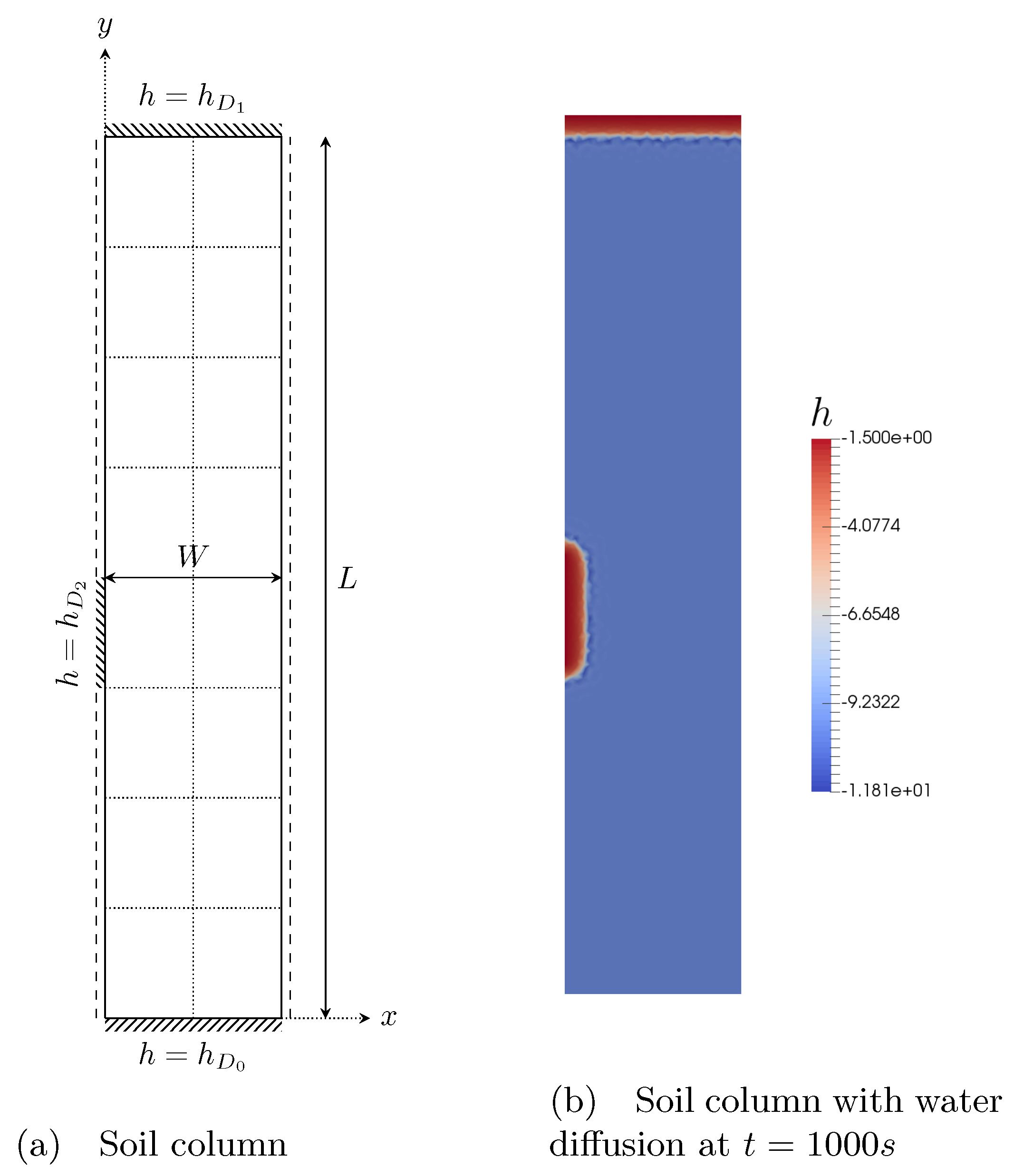
This test-case is inspired from the standard Polmann case [45,46]: the problem to be solved is the diffusion in two directions of water in a column of soil (see Figure 2a). The considered rectangular domain is $\mathsf{\Omega }=\left[0,W\right]\times \left[0,L\right]$. Geometrical parameters are given in

Table 1. Geometrical, Van Genuchten and load parameters for the soil column.

Geometrical Parameters [m]
L	1
W	0.2
Load Parameters [m]
$h_{D_0}$	−10
$h_{D_1}$	−1.5
$h_{D_2}$	−1.5
Van Genuchten Parameters
${\theta }_r$	0.368
${\theta }_s$	0.102
$K_s$	9.22 × 10${}^{-5}$ [m.s${}^{-1}$]
$\alpha$	3.35 [m${}^{-1}$]
n	2
m	0.5

. Initial pressure field is chosen to be homogeneous:

$$h(x,t<0)=h_{D_0}.$$

At time $t=0$, a pressure $h=h_{D_1}$ is imposed on the edge defined by $y=L$, and $h=h_{D_2}$ on the edge defined by $\left(x=0,y\in \left[3L/8;L/2\right]\right)$; the bottom edge $y=0$ is maintained at $h=h_{D_0}$. Remaining outer walls are chosen to be impermeable (null flow). Load parameters are also given on Table 1.

The Richards equation for water diffusion is considered here in its classical form:

$$\begin{array}{ccc}\hfill \mathrm{Find}\mathrm{scal}& \mathrm{ar}\mathrm{pressure}\mathrm{field}h(x,t)\mathrm{such}\mathrm{that}:\hfill & \hfill \frac{\partial \theta \left(h\right)}{\partial t}-\nabla ·\left(K\left(h\right)\nabla \left(h-z\right)\right),\end{array}$$

where:

• $\theta \left(h\right)$ is the volumetric water content: $\theta \left(h\right)={\theta }_r+\left({\theta }_s-{\theta }_r\right)S\left(h\right)$, with ${\theta }_r,{\theta }_s$ the residual and maximal water contents, and S the saturation degree.
• $K\left(h\right)$ is the soil hydraulic conductivity: $K\left(h\right)=K_s{K}_r\left(h\right)$, with $K_s,K_r$ the intrinsic and relative conductivities.

Van Genuchten model is used for the saturation degree and the relative conductivity:

$$\left\{\begin{array}{cc}\hfill & S\left(h\right)={\left(1+{\epsilon \left|h\right|}^n\right)}^{-m},\hfill \\ \hfill & K_r\left(h\right)={\left(1-{\left(\epsilon \left|h\right|\right)}^{n-1}{\left(1+{\left(\epsilon \left|h\right|\right)}^n\right)}^{-m}\right)}^2{\left(S\left(h\right)\right)}^{1/2},\hfill \end{array}\right.$$

with $\epsilon$ a scale parameter inversely proportional to the mean pore diameter. Material parameters are also given in Table 1.

Remark 8.

As all transient problems dealt with implicit time integration, the approximation of the Richards equation does not involve rigid body modes within subdomains. This leads to FETI bearing no natural coarse space. In order to ensure the scalability of the method, in a linearized context, an augmentation coarse space shall be added based on rigid body motions [47], another option would be to use GENEO modes or multipreconditioning [48].

Note that the absence of natural coarse space is correlated to the limited propagation of phenomena in a given time step (finite celerity of waves in the hyperbolic case or exponential decay in the parabolic case). Our approach which intensifies local computations, makes sense, even if in itself it can not cure the non-scalability. Coupling nonlinear preconditioning with augmentation or multipreconditioning will be the subject of future studies.

For the time integration, a simple discrete implicit Euler scheme is used with time step $\mathsf{\Delta }t$. Writing $h^n=h\left(x,t_n\right)$, one has:

$${\left.{\displaystyle \frac{\partial \theta \left(h\right)}{\partial t}}\right|}_{t=t_{n+1}}={\displaystyle \frac{\theta \left(h^{n+1}\right)-\theta \left(h^n\right)}{\mathsf{\Delta }t}}.$$

The time step is taken equal to: $\mathsf{\Delta }t=20s$.

Let $H_d^1\left(\mathsf{\Omega }\right)$ denote the subspace of square-integrable functions with square-integrable gradient which respect the given Dirichlet conditions, and let $H_0^1\left(\mathsf{\Omega }\right)$ be the associated vector space. The global nonlinear system to be solved on the whole domain $\mathsf{\Omega }$, at each time step, can be written as:

$$\begin{array}{cc}\hfill & \begin{array}{cc}\hfill \mathrm{Being}\mathrm{given}{h}^n& \in H_d^1\left(\mathsf{\Omega }\right),\mathrm{find}{h}^{n+1}\in H_d^1\left(\mathsf{\Omega }\right)\mathrm{such}\mathrm{that}\forall w\in H_0^1\left(\mathsf{\Omega }\right):\hfill \\ \hfill & {\mathcal{G}}_{int}\left(h^{n+1},w\right)+{\mathcal{G}}_{ext}\left(h^n,w\right)=0\hfill \end{array}\hfill \\ \hfill \mathrm{with}:& \left\{\begin{array}{cc}\hfill {\mathcal{G}}_{int}\left(h^{n+1},w\right)& \equiv {\int }_{\mathsf{\Omega }}{\displaystyle \frac{\partial \theta \left(h^{n+1}\right)}{\mathsf{\Delta }t}}wd\mathsf{\Omega }+{\int }_{\mathsf{\Omega }}K\left(h^{n+1}\right)\nabla h^{n+1}·\nabla wd\mathsf{\Omega }\hfill \\ & -{\int }_{\mathsf{\Omega }}K\left(h^{n+1}\right)\nabla y·\nabla wd\mathsf{\Omega }\hfill \\ \hfill {\mathcal{G}}_{ext}\left(h^n,w\right)& \equiv -{\int }_{\mathsf{\Omega }}{\displaystyle \frac{\theta \left(h^n\right)}{\mathsf{\Delta }t}}wd\mathsf{\Omega }=0.\hfill \end{array}\right.\hfill \end{array}$$

By choosing a discretization and applying the Finite Element theory to this system, one derives operators $g_{int}$ and $g_{ext}$ from ${\mathcal{G}}_{int}$ and ${\mathcal{G}}_{ext}$. The spatial discretization here involves 5244 degrees of freedom. The domain is split into 16 subdomains, leading to 333 interface degrees of freedom (see Figure 2a). The relative precision of each solver is set to ${\epsilon }_{rel}={10}^{-6}$, and absolute precision to ${\epsilon }_{abs}={10}^{-20}$.

Remark 9.

Richards equation is time-dependent, however our contribution is only related to the acceleration of nonlinear space problems, we thus focus on the solving of the nonlinear system produced at each step of the implicit integration Euler scheme.

Readers interested in the global performance of solving strategies, including in particular the treatment of time dependence, may refer to absolutely scalable algorithms as defined in [49,50]. Note that algorithms allowing local nonlinear resolutions were proved to improve the space scalability of certain nonlinear problems in [28].

The following three methods are compared: BDD-NL, FETI-NL and FETI-precNL. The comparison is performed on the number of iterations of the three nested solvers: global Newton iterations (cumulated over time steps), Krylov iterations (cumulated over global Newton iterations and time steps) and local Newton iterations (being given the parallelism of these solves, at each global Newton loop, the maximum over subdomains of local Newton iterations is stored; this value is then cumulated over global Newton iterations and time steps). The Krylov iterations are of particular importance since each of them is associated with two all-neighbors exchanges and at least one all-to-all reduction, which often affects the scalability of the methods. The results are given in

Table 2. Richards equation—global iterations.

# Global Newton Cumulated Iterations
Time	BDD-NL	FETI-NL	FETI-precNL	Gains of FETI-precNL (%)
				vs. BDD-NL	vs. FETI-NL
20	8	9	4	50	56
80	35	39	15	57	62
400	147	159	73	50	54
1000	311	325	179	42	45

,

Table 3. Richards equation—Krylov iterations.

# Krylov Cumulated Iterations
Time	BDD-NL	FETI-NL	FETI-precNL	Gains of FETI-precNL (%)
				vs. BDD-NL	vs. FETI-NL
20	32	37	16	50	57
80	157	169	65	59	62
400	715	714	338	53	53
1000	1535	1535	835	46	46

and

Table 4. Richards equation—local iterations.

# Local Newton Cumulated Iterations
Time	BDD-NL	FETI-NL	FETI-precNL	Ratios of FETI-precNL
				over BDD-NL	over FETI-NL
20	224	249	241	1,08	0,97
80	595	714	618	1,04	0,87
400	1576	2020	1981	1,26	0,98
1000	2559	3173	3608	1,41	1,14

. Figure 2b shows the state of the column after 1000 s.

On this problem, BDD-NL and FETI-NL methods were quite equivalent (see Table 2 and Table 3: at last time step, a total of 1535 cumulated Krylov iterations was recorded for both methods, while global Newton cumulated iterations numbers reached 311 and 325 for primal and dual approach, respectively), with a smaller local cost for primal approach (at the last time step, only 2559 cumulated local iterations were needed, versus 3173 for dual approach). FETI-precNL method was however way more efficient than these two approaches, with a total of only 179 cumulated global Newton iterations (see Table 2). The corresponding gains, in terms of global Newton iterations, compared to BDD-NL (resp. FETI-NL) method, range between 42% and 57% (resp. 45% and 62%) on the whole resolution. Regarding the Krylov cumulated iterations (see Table 3), the gains of FETI-precNL solver range between 46% and 59% versus primal approach, and vary from 46% to 62% compared to the dual approach. The gain of FETI-precNL solver, compared to BDD-NL and FETI-NL methods, depends on the intensity of the nonlinearity during each time step: as time increases, the speed of the diffusion decreases, resulting in a slow decrease of the FETI-precNL gain.

The cost of nonlinear preconditioning, i.e., additional local nonlinear iterations (in parallel), is evaluated in Table 4 by the ratios of the numbers of local Newton iterations for FETI-precNL compared to other methods: a maximal ratio of 1.41 is reached at the end of the resolution for BDD-NL method (1.14 for FETI-NL method). This additional cost is expected to be much less expensive than the decrease of about 50% in cumulated Krylov iterations (and the associated communications between processors).

A comparison is also made with classical NKS solving process with BDD algorithm as linear solver. Results are given in

Table 5. Richards equation—comparison with NKS method.

# Global Newton Cumulated Iterations
Time	NKS	FETI-precNL	Gains of FETI-precNL (%)
20	21	4	81
100	72	20	72
200	117	42	64
400	189	73	61
700	279	121	57
1000	368	179	51
# Krylov cumulated iterations
Time	NKS	FETI-precNL	Gains of FETI-precNL (%)
20	84	16	81
100	321	89	72
200	546	189	65
400	906	338	63
700	1356	573	58
1000	1801	835	54
# Local Newton cumulated iterations
Time	NKS	FETI-precNL	Ratio of FETI-precNL over NKS
20	22	241	10.95
100	77	769	9.99
200	127	1354	10.66
400	209	1981	9.48
700	314	2779	8.85
1000	418	3608	8.63

for the three involved algorithms (global Newton, Krylov and local Newton). For the classical NKS method, at each time step, the number of local Newton iterations is equal to the number of global Newton iterations plus one (the +1 is required to initialize the global solver). Gains range for global Newton and Krylov solver, between 51 and 82%, over the whole resolution. The ratio between (parallel) local Newton iterations is close to 10 at the beginning of the resolution and then slowly decreases, a cost which should be largely balanced by the 80% gain in the number of Krylov iterations (which involve communications between processors).

4.2. Nonlinear Thermal Problem

A second numerical test involves a symmetrized stationary nonlinear thermal behavior, described by the following partial differential equation in the domain $\mathsf{\Omega }$:

$$r_{vol}-\nabla ·\left(-K\left(T\right)\nabla T\right)=0,$$

with T the temperature, $r_{vol}$ a source of heat, and $K\left(T\right)$ the thermal conductivity. Nonlinearity comes from the dependence of K with respect to the temperature T, which is usually set to a linear or a power law:

$$K\left(T\right)=1+\alpha T\mathrm{or}K\left(T\right)={\left(1+T\right)}^{\alpha },$$

(38)

where $\alpha$ is a real number, parameter of the conductivity law. In the context of the nonlinear preconditioner for FETI-NL solver, in order to satisfy property (6), we chose a slightly different expression, where K depends on the gradient of T, in the spirit of linear elasticity:

$$K\left(T\right)={\left(1+\nabla T·\nabla T\right)}^{\alpha }.$$

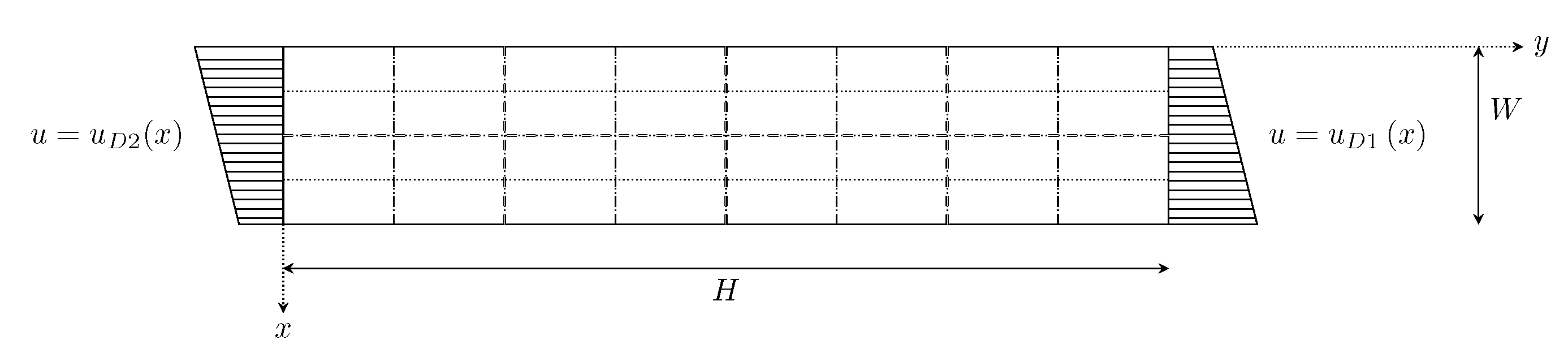
$\mathsf{\Omega }$ is a rectangular domain: $\mathsf{\Omega }=\left[0,L\right]\times \left[0,l\right]$, with Dirichlet boundary conditions (see Figure 3) on the left and right sides, and null flux condition on the top and bottom sides. Geometry and load parameters are given in

Table 6. Geometrical, material and load parameters: nonlinear thermal behavior.

Geometrical Parameters
H	1
W	0.2
Material parameters
$\alpha$	$\in \left\{0,0.2,0.4,0.6\right\}$
Load parameters
$u_{D1}\left(x\right)$	$10x+2$
$u_{D2}\left(x\right)$	$-10x+4$
$r_{vol}$	0

. Different levels of nonlinearity are considered, via an incremental variation of the parameter $\alpha$, which is sampled between $\alpha =0$ (linear case) and ${\alpha }_{max}=0.6$.

Using the same notations for the Sobolev subspace of admissible functions, the global nonlinear system to be solved on the whole domain $\mathsf{\Omega }$, at each time step, can eventually be written in weak form:

$$\begin{array}{cc}\hfill & \begin{array}{cc}\hfill \mathrm{Find}& T\in H^1\left(\mathsf{\Omega }\right)\mathrm{such}\mathrm{that}\forall w\in H_0^1\left(\mathsf{\Omega }\right):\hfill \\ \hfill & {\mathcal{G}}_{int}\left(T,w\right)+{\mathcal{G}}_{ext}\left(w\right)=0,\hfill \end{array}\hfill \\ \hfill \mathrm{with}:& \left\{\begin{array}{cc}\hfill {\mathcal{G}}_{int}\left(T,w\right)& \equiv -{\int }_{\mathsf{\Omega }}K\left(T\right)\nabla T·\nabla wd\mathsf{\Omega },\hfill \\ \hfill {\mathcal{G}}_{ext}\left(w\right)& \equiv {\int }_{\mathsf{\Omega }}{r}_{vol}wd\mathsf{\Omega }.\hfill \end{array}\right.\hfill \end{array}$$

By choosing a discretization and applying the Finite Element theory to this system, one derives operators $g_{int}$ and $g_{ext}$ from ${\mathcal{G}}_{int}$ and ${\mathcal{G}}_{ext}$.

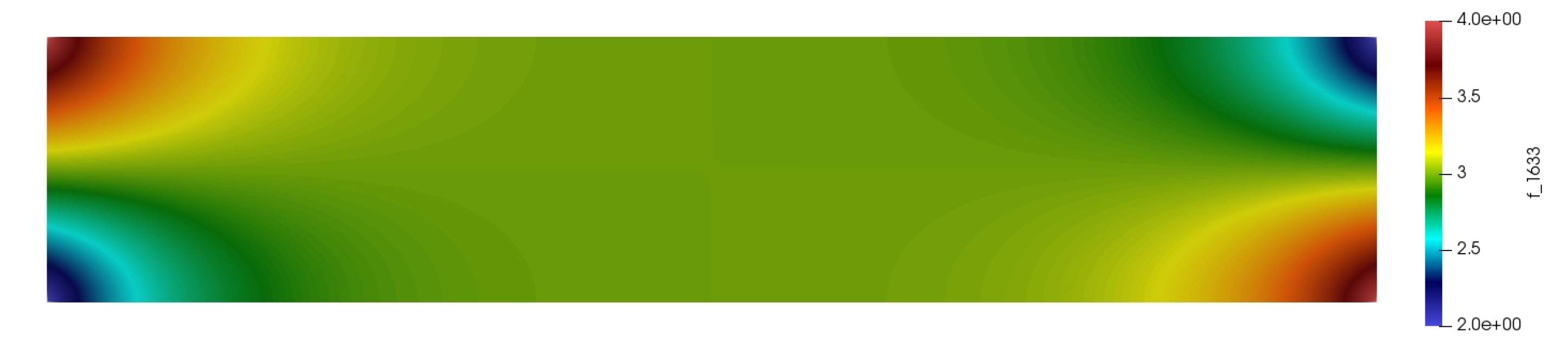
We tried to assess the (strong) scalability of the methods on this example. For the problem given in Table 6, we considered 3 different decompositions involving, respectively, 8 ($4\times 2$ subdomains, leading to a coarse space of dimension 4), 16 ($8\times 2$ subdomains, leading to a coarse space of dimension 12) and 32 subdomains ($8\times 4$ subdomains, leading to a coarse space of dimension 24), see Figure 3. To perform the three levels of substructuring, we use the same global mesh and refine only the substructuring. The global mesh is composed of 21,342 nodes and 43,959 elements. The solution map for $\alpha =6\times {10}^{-1}$ in presented of Figure 4.

We here used a synchronization of the stopping criteria of tangent solvers with the evolution of the global interface residual (see [40] for the general theory and [26] for its application in BDD-NL and FETI-NL), in order to avoid unnecessary iterations. Following common values and safeguards, we chose (the expression is given with FETI-precNL notations but equivalent methods were applied with other solvers):

$$\left\{\begin{array}{cc}\hfill & {\epsilon }_{K_k}=\gamma {\left(\frac{\parallel {\mathbf{h}}_{\mathbf{nl}}\left({{\lambda }_{\mathbf{b}}}_k\right)\parallel }{\parallel {\mathbf{h}}_{\mathbf{nl}}\left({{\lambda }_{\mathbf{b}}}_{k-1}\right)\parallel }\right)}^{\alpha }\mathrm{with}\gamma =0.7,\alpha =1.8,{\epsilon }_{K_0}={10}^{-2},\hfill \\ \hfill & \mathrm{if}\gamma {\epsilon }_{K_{k-1}}^{\alpha }>0.1:{\epsilon }_{K_k}=max\left\{{\epsilon }_{K_k},\gamma {\epsilon }_{K_{k-1}}^{\alpha }\right\},\hfill \\ \hfill & {\epsilon }_{K_k}=min\left\{{\epsilon }_{K_k},0.9\right\}.\hfill \end{array}\right.$$

(39)

For the 16 and 32 subdomains decompositions, we also defined a strategy where the nonlinear preconditioner was deactivated when the solver was “close to” convergence (this notion still needs an automatization procedure); this enabled to save local Newton iterations.

The numbers of iterations of the three nested solvers are compared for BDD-NL, FETI-NL and FETI-precNL methods: global Newton iterations (for each value of parameter $\alpha$), Krylov iterations (cumulated over global Newton loops) and local Newton iterations (cumulated over global Newton loops). Results are given in

Table 7. Nonlinear thermal behavior: global Newton and Krylov iterations.

# Global Newton Iterations
	BDD-NL			FETI-NL			FETI-precNL			Gains of FETI-precNL (%)
										vs. BDD-NL			vs. FETI-NL
#SD	8	16	32	8	16	32	8	16	32	8	16	32	8	16	32
$\alpha =0$	1	1	1	1	1	1	1	1	1	0	0	0	0	0	0
$\alpha =0.2$	6	6	7	5	6	5	3	3	4	50	50	43	40	50	20
$\alpha =0.4$	7	6	8	7	8	9	3	3	4	57	50	50	57	63	56
$\alpha =0.6$	7	6	8	8	7	9	4	4	5	43	33	38	50	43	44
# Krylov iterations
	BDD-NL			FETI-NL			FETI-precNL			Gains of FETI-precNL (%)
										vs. BDD-NL			vs. FETI-NL
#SD	8	16	32	8	16	32	8	16	32	8	16	32	8	16	32
$\alpha =0$	8	8	14	8	8	15	8	8	15	0	0	−6	0	0	0
$\alpha =0.2$	20	21	30	17	24	32	17	17	29	15	19	3	0	29	9
$\alpha =0.4$	22	22	31	20	25	40	16	15	27	27	32	13	20	40	33
$\alpha =0.6$	21	21	38	25	23	43	22	20	33	−5	5	13	12	13	23

and

Table 8. Nonlinear thermal behavior: local Newton iterations.

Max # Local Newton Iterations
	BDD-NL			FETI-NL			FETI-precNL			Ratio of FETI-precNL
										vs. BDD-NL			vs. FETI-NL
#SD	8	16	32	8	16	32	8	16	32	8	16	32	8	16	32
$\alpha =0$	1	1	1	1	1	1	2	2	2	2.	2.	2.	2.	2.	2.
$\alpha =0.2$	11	13	17	11	14	14	18	14	17	1.6	1.1	1	1.6	1	1.2
$\alpha =0.4$	15	15	29	18	20	33	22	18	20	1.5	1.2	1.1	1.2	0.9	0.6
$\alpha =0.6$	18	17	20	24	24	34	29	24	29	1.6	1.4	1.5	1.2	1	0.9

: the former presents the expected gains (reduction of global Newton and Krylov iterations), the latter gives the resulting costs (increase of local Newton computations).

We observe that FETI-precNL almost always behaves better than FETI-NL and BDD-NL. Furthermore, FETI-precNL seems to be less sensitive to the increase of the number of subdomains (at most 5 global Newton iterations are required to be compared with the 8 and 9 iterations for the other methods) and to the increase of the nonlinearity. In terms of communications (measured by the number of Krylov iterations), FETI-precNL needs, on average, 14% less exchanges than BDD-NL and 20% less exchanges than FETI-NL. The increase of the number of iterations between the 16- and 32-subdomain decompositions is a bit unexpected (but in that case the characteristic length of subdomains was not modified whereas the size of the interface was doubled); note that the increase is more moderate with FETI-precNL than with other approaches and even compared to the linear case. If we concentrate on the two finest decompositions (more relevant in the DD context), average gains are of 14 and 25% respectively. The extra-cost is limited since, on average, only 28% local solutions are needed compared to BDD-NL and 7% compared to FETI-NL.

5. Conclusions

This article investigates a new technique of preconditioning for FETI solver, in the context of the nonlinear substructuring and condensation method. A nonlinear version of the classical scaled Dirichlet preconditioner is built under the form of a nonlinear fixed point condensed system, in place of the classical FETI-NL nonlinear interface condensed problem. A global Newton algorithm is used to solve this new nonlinearly preconditioned interface problem, and tangent operators have the exact form of classical preconditioned projected FETI operators of which a good condition number can be expected. This solving process is called FETI-precNL. One iteration of FETI-precNL involves two times more local (fully parallel) nonlinear computations than other nonlinear domain decomposition methods like FETI-NL and BDD-NL. The hope is that this intensification of local computation gives better estimate of the actual state of the structure and limits the number of interface iterations which involve many communications and lower the parallel performance of the methods.

Numerical assessments on two small academic test cases show that interesting performance can be achieved with FETI-precNL method, when compared to BDD-NL and FETI-NL solvers. The first test case is a water diffusion problem in a soil column (which does not produce rigid body modes), and the second one a symmetrized nonlinear thermal case. For the first test, FETI-precNL method clearly performs better than BDD-NL and FETI-NL methods (gains are about 50%) in term of Krylov iterations, which are the more communication demanding steps of the domain decomposition algorithms. For the second test case, several decompositions were considered, for purposes of a strong scalability study: as expected, the performance of the solver does not collapse when the number of subdomains grows (although further analysis should assess the scalability of the solving process in a real High Performance Computing context). Moreover, average gains of 14 and 25% (compared to BDD-NL and FETI-NL, respectively) were achieved for the two finest decompositions. These first results are promising, and large scale implementation for mechanical problems is in progress.

In the future, we will try to port robustness-enhancing features which are necessary in order to tackle problems of industrial complexity. Anyhow adapted coarse spaces [10,12] add constraints that bend the search space into a manifold (instead of a vector space), which makes the nonlinear solving more complex. The idea of defining a nonlinear version of multipreconditioning [14] is seducing but far from simple either.

Furthermore, the ability to concentrate nonlinear computations at the scale of the subdomains triggers the difficulty of load balancing between processor. Note that one advantage of our approach is that subdomains not concerned by the nonlinearity have the possibility to idle and reduce their power consumption while waiting for the evolution of the nonlinear subdomains. This is to be compared with a classical approach where all subdomains need to compute tangent systems all the time even if their own computation does not contribute to the progress of the simulation which is driven by the localized nonlinearity. In the future, we will address the load balancing issue by using an adaptive approach: starting from coarse simulations, we should be able to adapt the discretization to the localization of errors, and to adapt the decomposition not only to the density of elements but also to the intensity of the nonlinearity. Another possibility will be to investigate asynchronous versions of our algorithms in the spirit of [51].

References

- Dryja, M.; Widlund, O. An Additive Variant of the Schwarz Alternating Method for the Case of Many Subregions; Department of Computer Science, Courant Institute: New York, NY, USA, 1987. [Google Scholar]
- Cai, X.C.; Sarkis, M. A restricted additive Schwarz preconditioner for general sparse linear systems. SIAM J. Sci. Comput. 1999, 21, 792–797. [Google Scholar] [CrossRef] [Green Version]
- Farhat, C.; Roux, F.X. A method of finite element tearing and interconnecting and its parallel solution algorithm. Int. J. Numer. Methods Eng. 1991, 32, 1205–1227. [Google Scholar] [CrossRef]
- Mandel, J. Balancing domain decomposition. Commun. Numer. Methods Eng. 1993, 9, 233–241. [Google Scholar] [CrossRef]
- Farhat, C.; Lesoinne, M.; LeTallec, P.; Pierson, K.; Rixen, D. FETI-DP: A dual-primal unified FETI method—Part I: A faster alternative to the two-level FETI method. Int. J. Numer. Methods Eng. 2001, 50, 1523–1544. [Google Scholar] [CrossRef]
- Dohrmann, C.R. A preconditioner for substructuring based on constrained energy minimization. SIAM J. Sci. Comput. 2003, 25, 246–258. [Google Scholar] [CrossRef]
- Gander, M.J.; Zhang, H. Optimized interface preconditioners for the FETI method. In Domain Decomposition Methods in Science and Engineering XXI; Springer: Berlin, Germany, 2014; Volume 98, pp. 657–665. [Google Scholar]
- Roux, F.X.; Magoulès, F.; Series, L.; Boubendir, Y. Approximation of optimal interface boundary conditions for two-Lagrange multiplier FETI method. In Domain Decomposition Methods in Science and Engineering; Springer: Berlin, Germany, 2005; Volume 40, pp. 283–290. [Google Scholar]
- Efendiev, Y.; Galvis, J.; Lazarov, R.; Willems, J. Robust domain decomposition preconditioners for abstract symmetric positive definite bilinear forms. ESAIM Math. Model. Numer. Anal. 2012, 46, 1175–1199. [Google Scholar] [CrossRef] [Green Version]
- Spillane, N.; Rixen, D.J. Automatic spectral coarse spaces for robust FETI and BDD algorithms. Internat. J. Num. Meth. Engin. 2013, 95, 953–990. [Google Scholar] [CrossRef]
- Beirão da Veiga, L.; Pavarino, L.F.; Scacchi, S.; Widlund, O.B.; Zampini, S. Isogeometric BDDC preconditioners with deluxe scaling. SIAM J. Sci. Comput. 2014, 36, A1118–A1139. [Google Scholar] [CrossRef] [Green Version]
- Klawonn, A.; Radtke, P.; Rheinbach, O. FETI-DP Methods with an Adaptive Coarse Space. SIAM J. Numer. Anal. 2015, 53, 297–320. [Google Scholar] [CrossRef]
- Bridson, R.; Greif, C. A multipreconditioned conjugate gradient algorithm. SIAM J. Matrix Anal. Appl. 2006, 27, 1056–1068. [Google Scholar] [CrossRef] [Green Version]
- Gosselet, P.; Rixen, D.; Roux, F.X.; Spillane, N. Simultaneous-FETI and Block-FETI: Robust domain decomposition with multiple search directions. Int. J. Numer. Methods Eng. 2015, 104, 905–927. [Google Scholar] [CrossRef] [Green Version]
- Cools, S.; Vanroose, W. The communication-hiding pipelined BiCGstab method for the parallel solution of large unsymmetric linear systems. Parallel Comput. 2017, 65, 1–20. [Google Scholar] [CrossRef] [Green Version]
- Cai, X.C.; Gropp, W.D.; Keyes, D.E.; Tidriri, M.D. Newton-Krylov-Schwarz methods in CFD. In Numerical Methods for the Navier–Stokes Equations; Springer: Berlin, Germany, 1994; pp. 17–30. [Google Scholar]
- Bhardwaj, M.; Day, D.; Farhat, C.; Lesoinne, M.; Pierson, K.; Rixen, D. Application of the FETI Method to ASCI Problems: Scalability Results on One Thousand Processors and Discussion of Highly Heterogeneous Problems; Technical Report; Sandia National Labs.: Albuquerque, NM, USA; Livermore, CA, USA, 1999. [Google Scholar]
- Biros, G.; Ghattas, O. Inexactness issues in the Lagrange-Newton-Krylov-Schur method for PDE-constrained optimization. In Large-Scale PDE-Constrained Optimization; Springer: Berlin, Germany, 2003; pp. 93–114. [Google Scholar]
- Klawonn, A.; Lanser, M.; Rheinbach, O.; Wellein, G.; Wittmann, M. Energy efficiency of nonlinear domain decomposition methods. Int. J. High Perform. Comput. Appl. 2021, 35, 237–253. [Google Scholar] [CrossRef]
- Cai, X.C.; Keyes, D.E. Nonlinearly preconditioned inexact Newton algorithms. SIAM J. Sci. Comput. 2002, 24, 183–200. [Google Scholar] [CrossRef] [Green Version]
- Marcinkowski, L.; Cai, X.C. Parallel Performance of Some Two-Level ASPIN Algorithms. In Domain Decomposition Methods in Science and Engineering; Kornhuber, R., Hoppe, R., Périaux, J., Pironneau, O., Widlund, O., Xu, J., Eds.; Springer: Berlin, Heidelberg, 2005; Volume 40, pp. 639–646. [Google Scholar]
- Dolean, V.; Gander, M.J.; Kheriji, W.; Kwok, F.; Masson, R. Nonlinear preconditioning: How to use a nonlinear Schwarz method to precondition Newton’s method. SIAM J. Sci. Comput. 2016, 38, A3357–A3380. [Google Scholar] [CrossRef] [Green Version]
- Heinlein, A.; Lanser, M. Additive and Hybrid Nonlinear Two-Level Schwarz Methods and Energy Minimizing Coarse Spaces for Unstructured Grids. SIAM J. Sci. Comput. 2020, 42, A2461–A2488. [Google Scholar] [CrossRef]
- Ladevèze, P.; Néron, D.; Gosselet, P. On a mixed and multiscale domain decomposition method. Comput. Methods Appl. Mech. Eng. 2007, 196, 1526–1540. [Google Scholar] [CrossRef] [Green Version]
- Gosselet, P.; Blanchard, M.; Allix, O.; Guguin, G. Non-invasive global-local coupling as a Schwarz domain decomposition method: Acceleration and generalization. Adv. Model. Simul. Eng. Sci. 2018, 5. [Google Scholar] [CrossRef] [Green Version]
- Negrello, C.; Gosselet, P.; Rey, C.; Pebrel, J. Substructured formulations of nonlinear structure problems-influence of the interface condition. Int. J. Numer. Methods Eng. 2016, 107, 1083–1105. [Google Scholar] [CrossRef] [Green Version]
- Negrello, C.; Gosselet, P.; Rey, C. A new impedance accounting for short and long range effects in mixed substructured formulations of nonlinear problems. Int. J. Numer. Methods Eng. 2017, 114, 675–693. [Google Scholar] [CrossRef]
- Klawonn, A.; Lanser, M.; Rheinbach, O. Nonlinear FETI-DP and BDDC Methods. SIAM J. Sci. Comput. 2014, 36, A737–A765. [Google Scholar] [CrossRef]
- Hinojosa, J.; Allix, O.; Guidault, P.A.; Cresta, P. Domain decomposition methods with nonlinear localization for the buckling and post-buckling analyses of large structures. Adv. Eng. Softw. 2014, 70, 13–24. [Google Scholar] [CrossRef]
- Klawonn, A.; Lanser, M.; Rheinbach, O.; Uran, M. New Nonlinear FETI-DP Methods Based on a Partial Nonlinear Elimination of Variables. In Proceedings of the 23rd International Conference on Domain Decomposition Methods, Jeju Island, Korea, 5–10 July 2015; Springer: Berlin, Germany, 2017; Volume 116, pp. 207–215. [Google Scholar]
- Klawonn, A.; Lanser, M.; Rheinbach, O.; Uran, M. Nonlinear FETI-DP and BDDC Methods: A Unified Framework and Parallel Results. SIAM J. Sci. Comput. 2017, 39, C417–C451. [Google Scholar] [CrossRef] [Green Version]
- Ciarlet, P.G. Linear and Nonlinear Functional Analysis with Applications; Society for Industrial and Applied Mathematics: Philadelphia, PA, USA, 2013. [Google Scholar]
- Brune, P.R.; Knepley, M.G.; Smith, B.F.; Tu, X. Composing scalable nonlinear algebraic solvers. SIAM Rev. 2015, 57, 535–565. [Google Scholar] [CrossRef] [Green Version]
- Agoshkov, V.I. Poincaré-Steklov’s operators and domain decomposition methods in finite dimensional spaces. In Proceedings of the First International Symposium on Domain Decomposition Methods for Partial Differential Equations, Paris, France, 7–9 January 1987; SIAM: Paris, France, 1988; pp. 73–112. [Google Scholar]
- Klawonn, A.; Widlund, O.B. FETI and Neumann-Neumann iterative substructuring methods: Connections and new results. Commun. Pure Appl. Math. 2001, 54, 57–90. [Google Scholar] [CrossRef]
- Gosselet, P.; Rey, C.; Rixen, D. On the initial estimate of interface forces in FETI methods. Comput. Methods Appl. Mech. Eng. 2003, 192, 2749–2764. [Google Scholar] [CrossRef] [Green Version]
- Parret-Fréaud, A.; Rey, V.; Gosselet, P.; Rey, C. Improved recovery of admissible stress in domain decomposition methods—Application to heterogeneous structures and new error bounds for FETI-DP. Int. J. Numer. Methods Eng. 2016. [Google Scholar] [CrossRef]
- Farhat, C.; Mandel, J. The two-level FETI method for static and dynamic plate problems Part I: An optimal iterative solver for biharmonic systems. Comput. Methods Appl. Mech. Eng. 1998, 155, 129–151. [Google Scholar] [CrossRef]
- Klawonn, A.; Lanser, M.; Rheinbach, O.; Uran, M. On the Accuracy of the Inner Newton Iteration in Nonlinear Domain Decomposition. In Domain Decomposition Methods in Science and Engineering XXIV; Bjørstad, P.E., Brenner, S.C., Halpern, L., Kim, H.H., Kornhuber, R., Rahman, T., Widlund, O.B., Eds.; Springer International Publishing: Cham, Switzerland, 2018; pp. 435–443. [Google Scholar]
- Eisenstat, S.C.; Walker, H.F. Choosing the forcing terms in an inexact Newton method. SIAM J. Sci. Comput. 1996, 17, 16–32. [Google Scholar] [CrossRef]
- Rixen, D.J.; Farhat, C. A simple and efficient extension of a class of substructure based preconditioners to heterogeneous structural mechanics problems. Int. J. Numer. Methods Eng. 1999, 44, 489–516. [Google Scholar] [CrossRef]
- Toselli, A.; Widlund, O. Domain Decomposition Methods—Algorithms and Theory; Springer Series in Computational Mathematics; Springer: Berlin/Heidelberg, Germany, 2005; Volume 34. [Google Scholar] [CrossRef]
- Alnæs, M.; Blechta, J.; Hake, J.; Johansson, A.; Kehlet, B.; Logg, A.; Richardson, C.; Ring, J.; Rognes, M.E.; Wells, G.N. The FEniCS project version 1.5. Arch. Numer. Softw. 2015, 3, 9–23. [Google Scholar]
- Geuzaine, C.; Remacle, J.F. Gmsh: A 3-D finite element mesh generator with built-in pre-and post-processing facilities. Int. J. Numer. Methods Eng. 2009, 79, 1309–1331. [Google Scholar] [CrossRef]
- Celia, M.A.; Bouloutas, E.T.; Zarba, R.L. A general mass-conservative numerical solution for the unsaturated flow equation. Water Resour. Res. 1990, 26, 1483–1496. [Google Scholar] [CrossRef]
- Sochala, P. Méthodes Numériques pour les Écoulements Souterrains et Couplage avec le Ruissellement. Ph.D. Thesis, École Nationale des ponts et Chaussées, Marne-la-Vallée, France, 2008. [Google Scholar]
- Farhat, C.; Chen, P.; Mandel, J. A scalable Lagrange multiplier based domain decomposition method for implicit time-dependent problems. Int. J. Numer. Methods Eng. 1995, 38, 3831–3858. [Google Scholar] [CrossRef]
- Leistner, M.C.; Gosselet, P.; Rixen, D.J. Recycling of Solution Spaces in Multi-Preconditioned FETI Methods Applied to Structural Dynamics. Int. J. Numer. Methods Eng. 2018. [Google Scholar] [CrossRef]
- Kanapady, R.; Tamma, K. A-scalability and an integrated computational technology and framework for non-linear structural dynamics. Part 1: Theoretical developments and parallel formulations. Int. J. Numer. Methods Eng. 2003, 58, 2265–2293. [Google Scholar] [CrossRef]
- Kanapady, R.; Tamma, K. A-scalability and an integrated computational technology and framework for non-linear structural dynamics. Part 2: Implementation aspects and parallel performance results. Int. J. Numer. Methods Eng. 2003, 58, 2295–2323. [Google Scholar] [CrossRef]
- Magoulès, F.; Szyld, D.B.; Venet, C. Asynchronous optimized Schwarz methods with and without overlap. Numer. Math. 2017, 137, 199–227. [Google Scholar] [CrossRef]
Figure 1.
Local numbering, interface numbering, trace and assembly operators.
Figure 2.
Richards equation: soil column with water diffusion in two directions.