An Analytical Expression for Magnet Shape Optimization in Surface-Mounted Permanent Magnet Machines


Department of Mechanical Engineering, Faculty of Engineering, Arak University, Arak 38156-8-8849, Iran
Math. Comput. Appl. 2018, 23(4), 57; https://0-doi-org.brum.beds.ac.uk/10.3390/mca23040057
Submission received: 16 July 2018
/
Revised: 2 October 2018
/
Accepted: 2 October 2018
/
Published: 5 October 2018
(This article belongs to the Special Issue Mathematical Models for the Design of Electrical Machines)
Abstract
:Surface-mounted permanent magnet machines are widely used in low and medium speed applications. Pulsating torque components is the most crucial challenge, especially in low-speed applications. Magnet pole shape optimization can be used to mitigate these components. In this research, an analytical model is proposed to calculate the magnetic vector potential in surface-mounted permanent magnet machines. A mathematical expression is also derived for optimal the magnet shape to reduce the cogging torque and electromagnetic torque components. The presented model is based on the resolution of the Laplace’s and Poisson’s equations in polar coordinates by using the subdomain method and applying hyperbolic functions. The proposed method is applied to the performance computation of a surface-mounted permanent magnet machine, i.e., a 3-phase 12S-10P motor. The analytical results are validated through the finite element analysis (FEA) method.
1. Introduction
Surface-mounted permanent magnet machines are interested in high-performance applications because of their high efficiency and power density. However, the noise and vibration caused by pulsating torque components seriously affect the machine performance. Pulsating torque is greatly affected by the distribution of the magnetic field and the configuration of the permanent magnets. Therefore, pulsating torque mitigation can be performed using magnet shape optimization to obtain a better magnetic field waveform and also to reduce the cogging torque and electromagnetic torque, effectively.
An extensive variety of techniques such as magnet skewing [1,2,3,4], magnet-arc optimization [5,6,7,8,9], magnet shape optimization [10], and magnet displacing [2,3,4,7,8,9] for minimizing cogging torque in permanent magnet motors is documented in the literature.
A variety of techniques including analytical and numerical methods have been conducted to evaluate the pulsating torque components in electrical machines. Numerical methods like the finite element method (FEA) give accurate results and are time-consuming especially in the first step of the design stage. Semi-analytical methods including conformal mapping [11,12,13,14] and Magnetic Equivalent Circuit (MEC) [15,16,17], and analytical methods including the subdomain model [18,19,20,21,22,23,24,25,26,27,28,29,30,31,32,33] are reported to model electrical machines and are useful in the design optimization stage. The subdomain model is more accurate than the other analytical models [15].
Indeed, the global or local saturation effect influences the electromagnetic performances, e.g., on the ripple/cogging torque [34]. To overcome that issue, recently, a new technique to account for finite soft-magnetic material permeabilities in the subdomain technique was developed by applying the superposition principle in both directions in polar or Cartesian coordinates [35,36]. According to Reference [37], the Dubas’ superposition technique [35,36] is very interesting since it enables the magnetic field calculation in the material of slotted geometries. This technique has been implemented in radial-flux electrical machines considering finite soft-magnetic material permeability [34]. The Dubas’s superposition technique could have been used to develop a new model with the consideration of the saturation effect. In References [38,39,40,41], an analytical model has been introduced to compute electric machine performance by using the subdomain method.
However, no analytical expression was found at present to calculate the optimal magnet pole shape in surface-mounted permanent magnet machines in order to minimize the pulsating torque components.
The focus of this paper is to derive an analytical expression for the optimal magnet pole shape in surface-mounted permanent magnet machines to reduce pulsating torque components. An analytical model is presented based on the resolution of the Laplace’s and Poisson’s equations in surface-mounted permanent magnet machines by using the subdomain method whilst considering pole shape optimization. It is shown that the developed model can effectively estimate the magnetic field, cogging torque, electromagnetic torque, back electromotive force and self/mutual inductance. This model is applied to the performance calculation of a surface-mounted permanent magnet motor, i.e., a 3-phase 12S-10P motor. It is shown that the results of the analytical model are in close agreement with the results of the FEA method.
2. Subdomain Definition
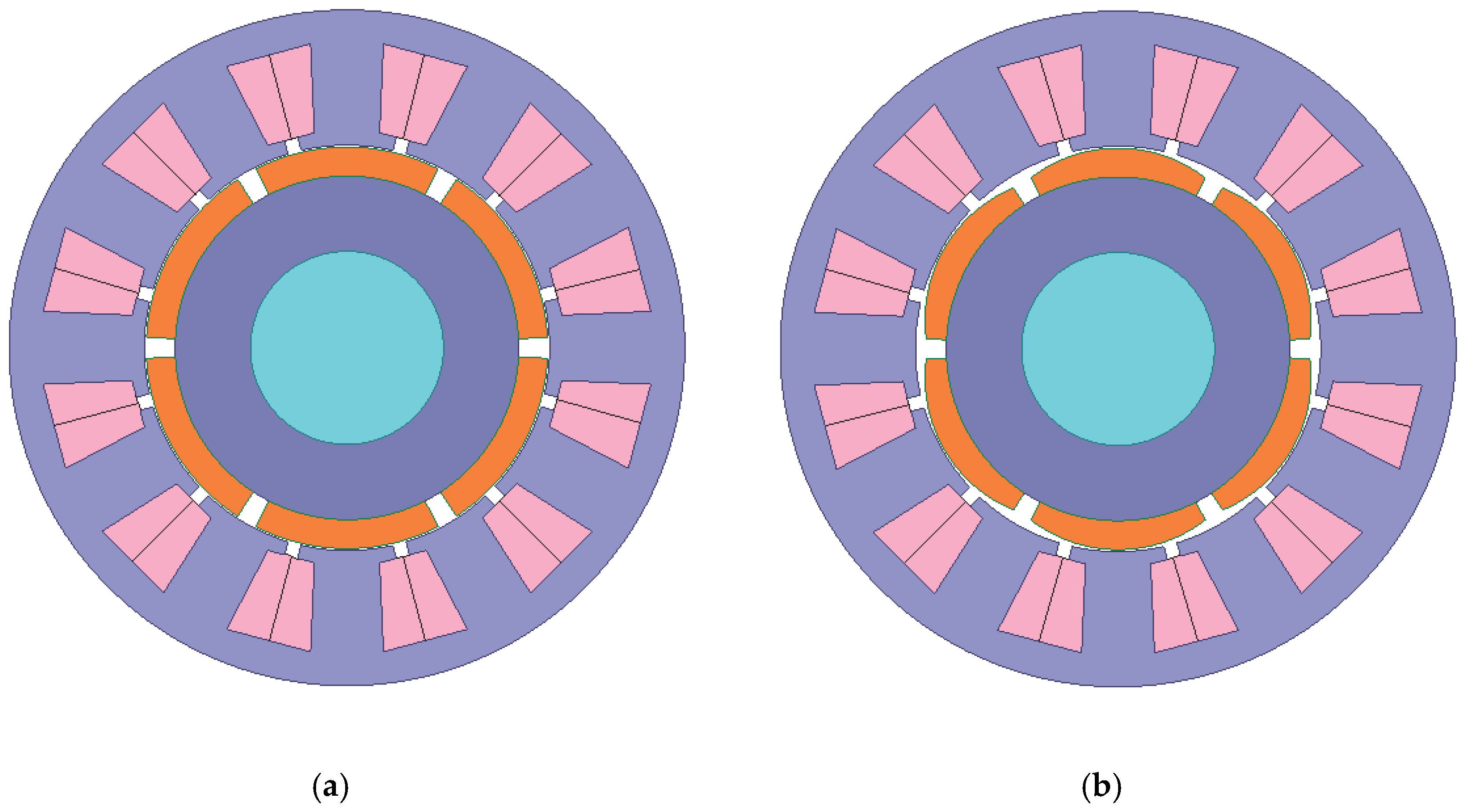
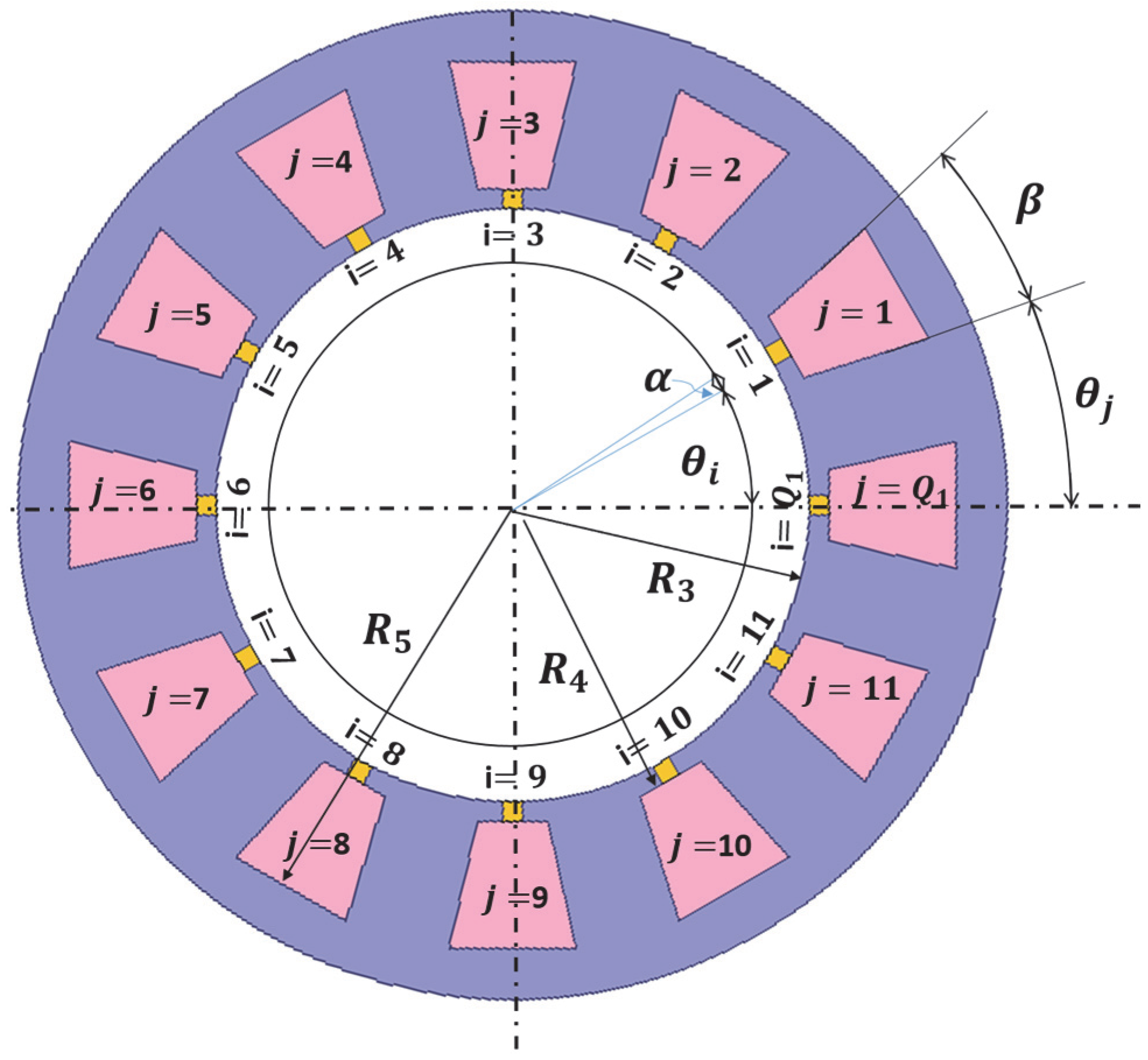
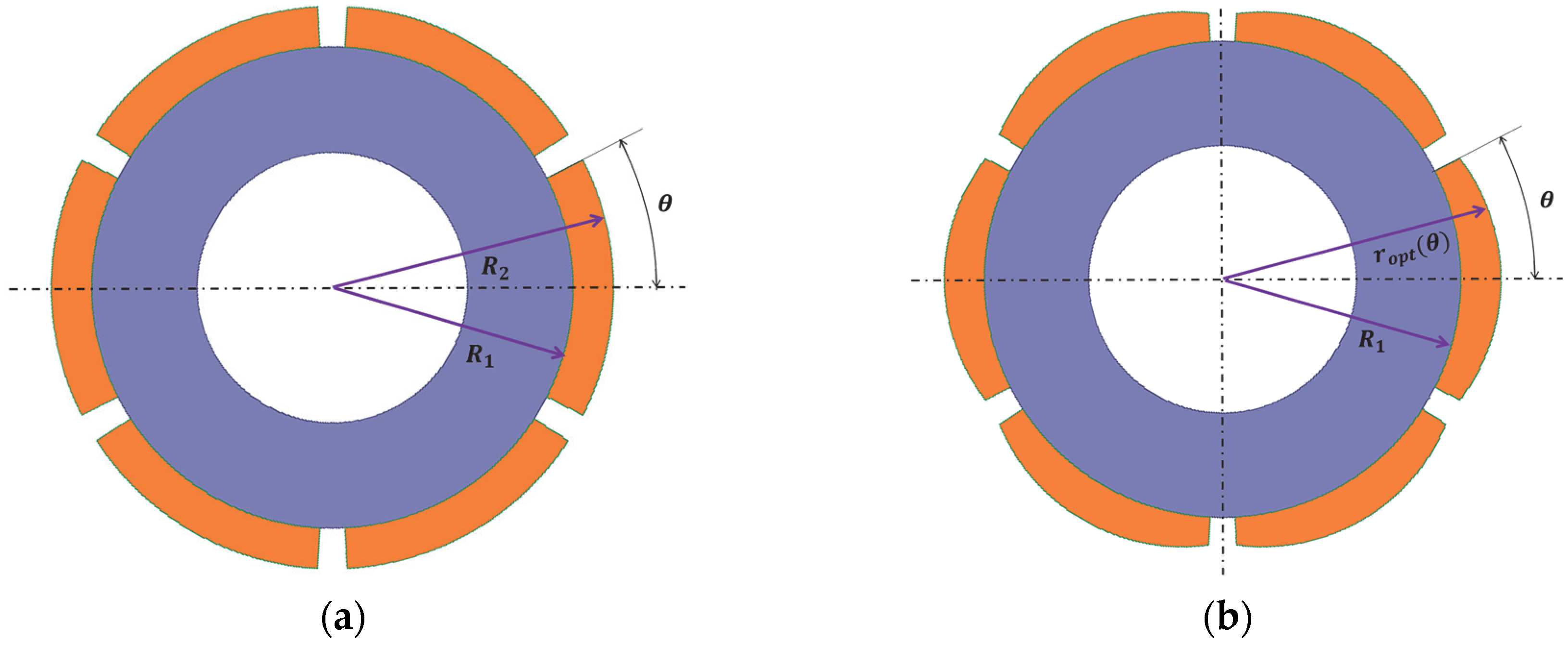
The schematic representation of the investigated machines is shown in Figure 1. The machine model is divided into four subdomains. The stator which has two subdomains including the slot regions (domain ), the slot opening regions (domain ) and the airgap subdomain (region ) are shown in Figure 2. The rotor has one subdomain including the permanent magnet regions (domain ), as shown in Figure 3.
The angular position of the -th stator slot and -th stator slot opening are defined as (1) and (2), respectively.
3. Magnetic Vector Potential Computation
The general solution to Laplace’s or Poisson’s equations in each subdomain is developed in this section. The Laplace equation can be described in the polar form as
By replacing by , one obtains
The 2D analytical model in quasi-Cartesian coordinates is formulated with the following assumptions:
- The end effects are neglected (i.e., the machine is infinitely long: the magnetic variables are independent of z).
- The stator is assumed to be infinitely permeable (i.e., the saturation effect is neglected) with zero electrical conductivity.
- The relative magnetic permeability and electrical conductivity of the solid rotor and shaft are assumed to be constant.
- The current density in the slots has only one component along the z-axis.
3.1. Magnetic Vector Potential in the Stator Slot Subdomain (Region j)
The Poisson equation in the stator slot subdomain is given by
where , and is the slot current density.
The Neumann boundary conditions at the bottom and at each side of the slot are obtained as
The general solution of Equation (5) using the separation of variables method is given by
where is a positive integer and the coefficients and are determined based on the continuity and interface conditions.
The continuity of the magnetic vector potential between the subdomain and the region leads to
The interface condition (9) gives
3.2. Magnetic Vector Potential in the Stator Slot Opening Subdomain (Region i)
The Laplace equation in the stator second inner slot opening subdomain is given by
where and .
The Neumann boundary conditions at the bottom and at each side of the slot are obtained as
The general solution of Equation (12) using the separation of variables method is given by
where is a positive integer and the coefficients, , , and are determined based on the continuity and interface conditions.
The continuity of the magnetic vector potential between the subdomain and the regions and leads to
The interface condition (15) gives
The interface condition (16) gives
3.3. Magnetic Vector Potential in the Air-Gap Subdomain (Region II)
The Laplace equation in the air-gap subdomain is given by
where and .
The general solution of Equation (21), considering the periodicity boundary conditions is obtained as
where is a positive integer.
The coefficients , , and are determined by considering the continuity of the magnetic vector potential between the internal airgap subdomain II and the region i using a Fourier series expansion of interface condition (23) and (24) over the airgap interval.
The continuity of the magnetic vector potential between the internal airgap subdomain and the regions and leads to
The interface condition (23) gives
The interface condition (24) gives
3.4. Magnetic Vector Potential in the Rotor Permanent Magnet Subdomain (Region I)
The Poisson equation in the rotor permanent magnet subdomain is given by
where and , and are the tangential and radial components of magnetization.
3.4.1. Radial Magnetization
The radial and tangential components of radial magnetization for the surface-mounted design can be expressed as
where is the magnet pole width to magnet pitch ratio.
3.4.2. Parallel Magnetization
The radial and tangential components of the parallel magnetization for the surface-mounted design can be expressed as
where
For a surface-mounted design, the Neumann boundary conditions at the bottom of the permanent magnet are obtained as
The general solution of Equation (29) using the separation of variables method is given by
where is a positive integer and the coefficients and are determined based on the continuity and interface conditions.
The continuity of the magnetic vector potential between the subdomain and the regions leads to
The interface condition (40) gives
4. Magnet Pole Shape Optimization
The general solution for the magnetic potential distribution in the air-gap subdomain is
The normal flux density is defined as
As the permeability of the stator/rotor iron core is much larger than that of air, the following boundary conditions are employed
- The scalar magnetic potential is expressed as in the inner stator surfaceor
- The normal flux density waveforms is sinusoidal in the inner stator surface and expressed as . Therefore,or
From the boundary conditions (46) and (48), we can get
At the position of , the magnetic potential is expressed as
or
In the outer surface of the rotor, the magnetic potential can be derived as
or
or
or
Therefore, the optimum magnet radii can be expressed as
5. Performance Calculation
The electromagnetic torque is obtained using the Maxwell stress tensor and expressed as
where is the axial length of the motor and is calculated by
The final expression of the electromagnetic torque can be expressed as
where,
For single layer winding, the phase flux vector is calculated by
where is the number of conductors in the stator slot, C is a matrix connection between the stator slots and phase connections, and is the slot flux.
For the stator slots, is given by
where is the stator fill factor and is the area of the stator slot.
For double-layer winding, the phase flux vector is calculated by
where
and
For the stator slots, is given by
The back-EMF of phase A is given by
where is the rotor angular speed and is the flux linkage per phase A.
The stator inductance (self-inductance) of phase A is given by
where is the peak current in phase A.
The mutual inductance of phase A and phase B is given by
where is the number of phase turns, is magnetic flux in phase A, and is the peak current in phase B.
6. Model Evaluation
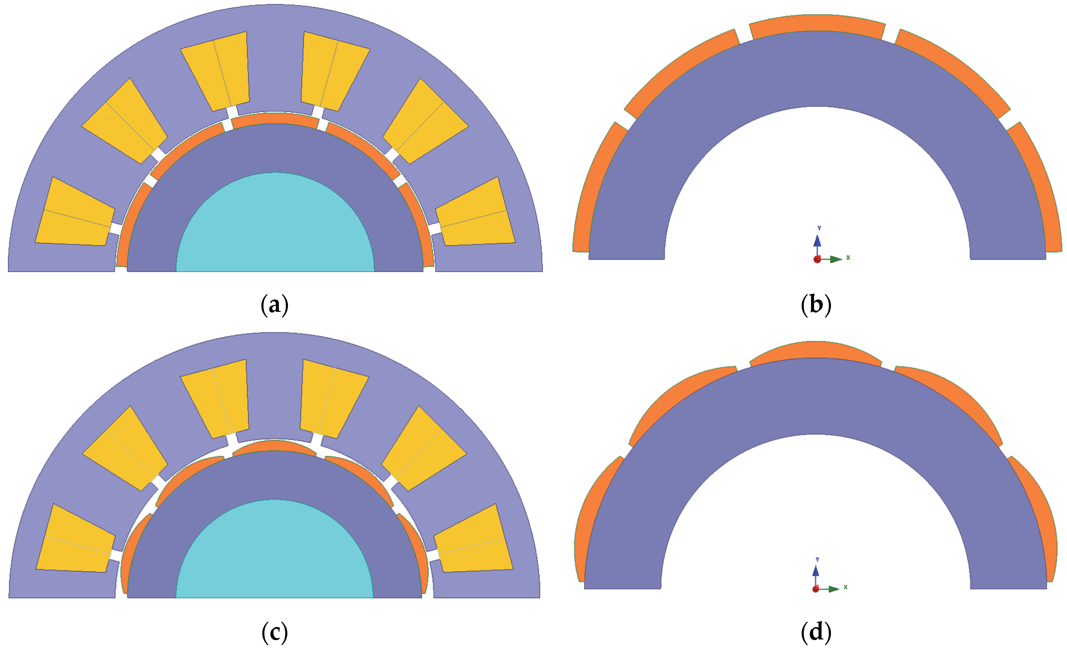
In this section, the presented analytical model is used to study the magnetic flux density, electromagnetic torque, and back-electromotive force of a 12S-10P motor. The results of the analytical method are then verified by the results of the finite element method. A 2D model of the studied brushless permanent magnet motor is shown in Figure 4 and the motor parameters are given in Table 1. The PM magnetization is radial. The slot contains two coils as shown in Figure 4a. In order to have a good precision in the analytical evaluation, the number of harmonic terms used in the computations is equal to 50 (air-gap and PM subdomains) and 30 (slots and slot-opening subdomain).
We have to solve a system of linear equations with the same number of unknowns (i.e., 12). The matrix connection between the stator slots and phase connections of each layer for the investigated motor are given by
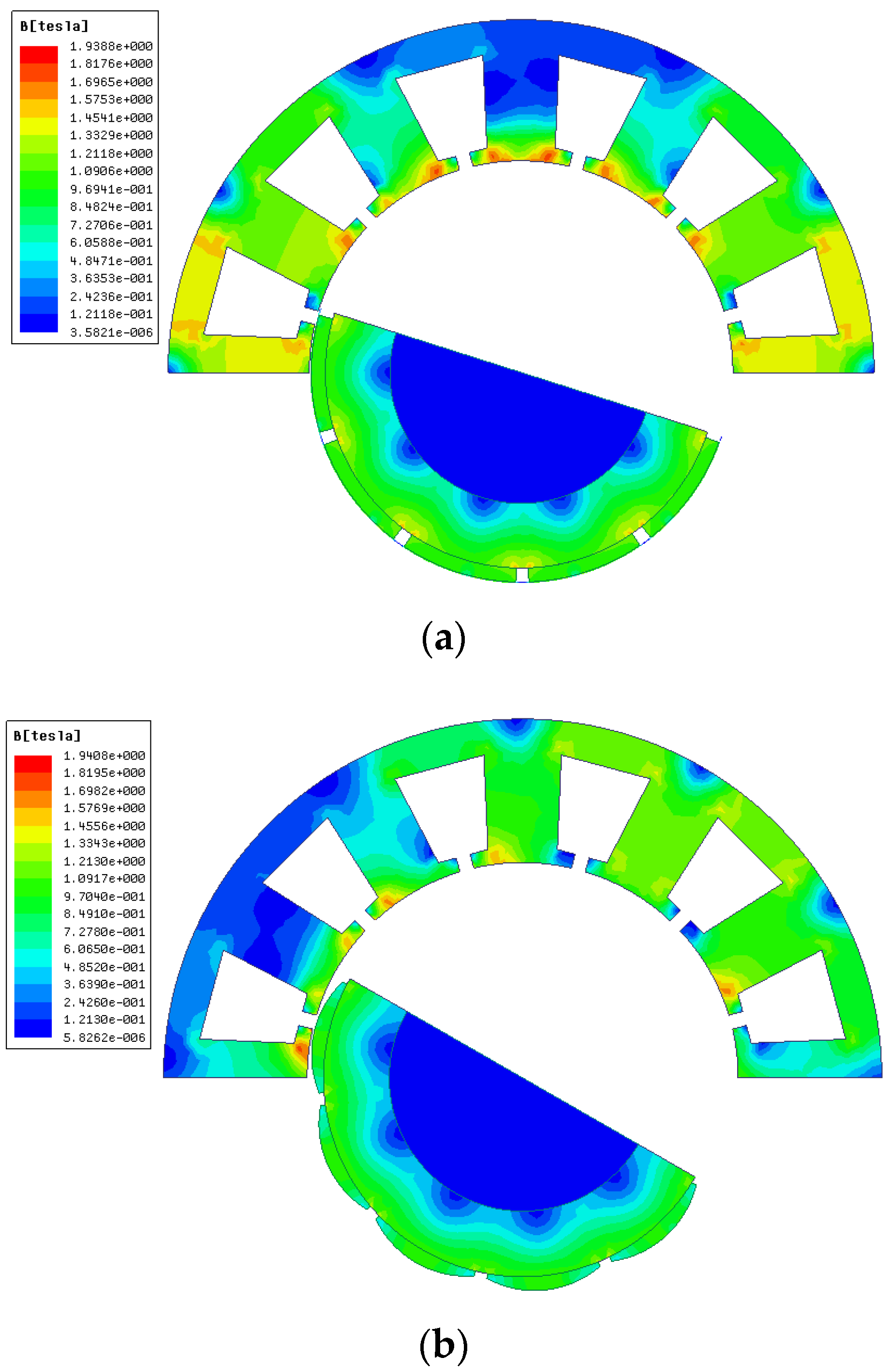
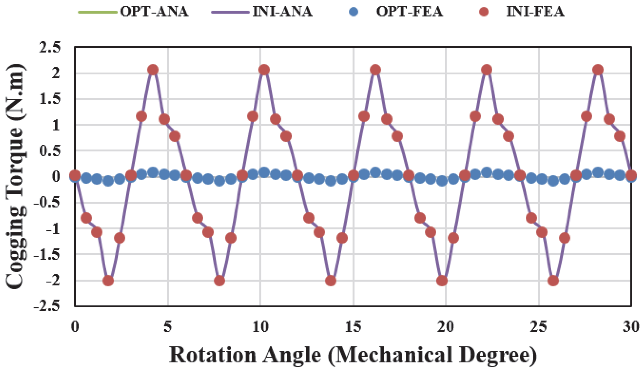
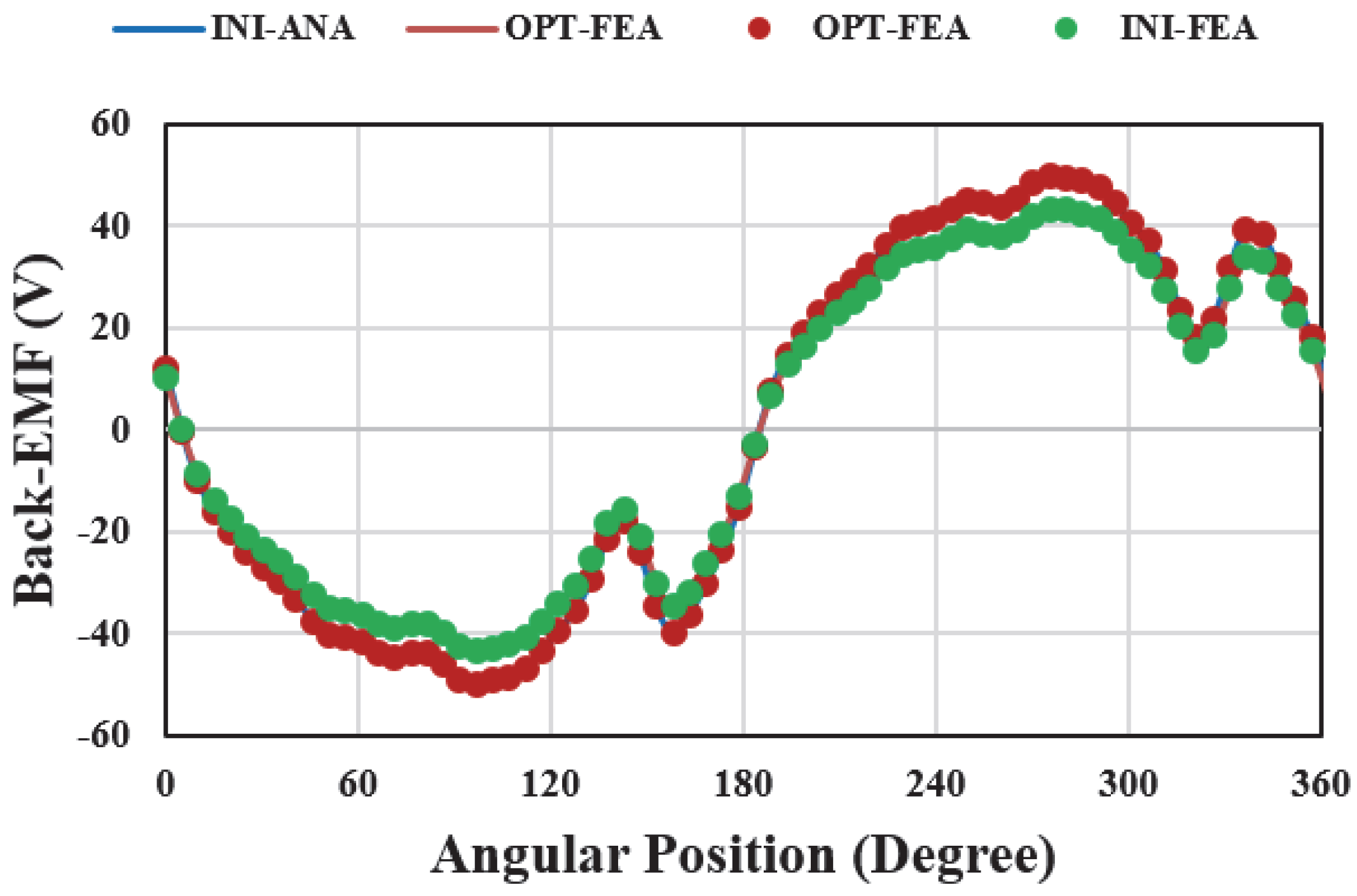
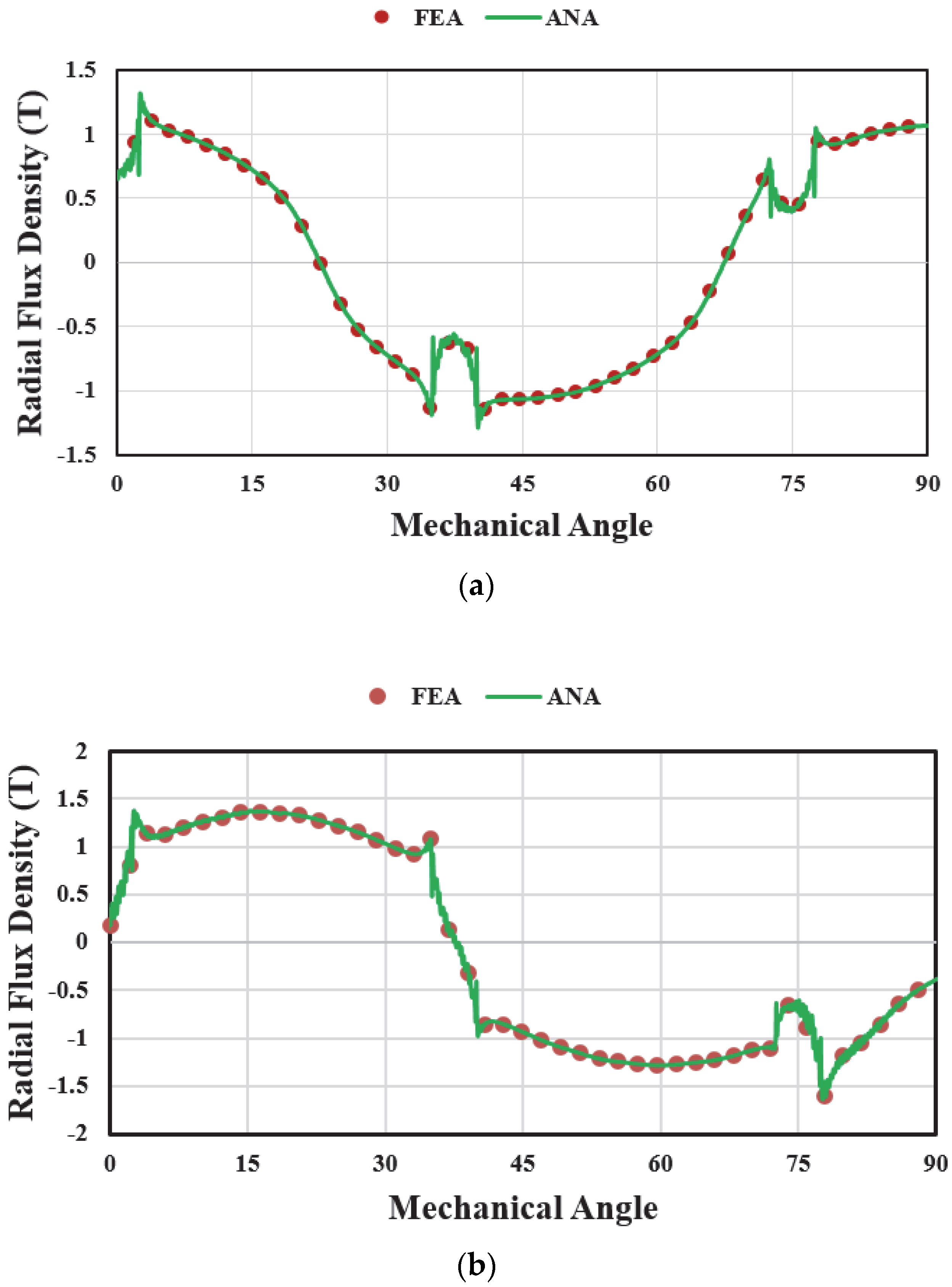
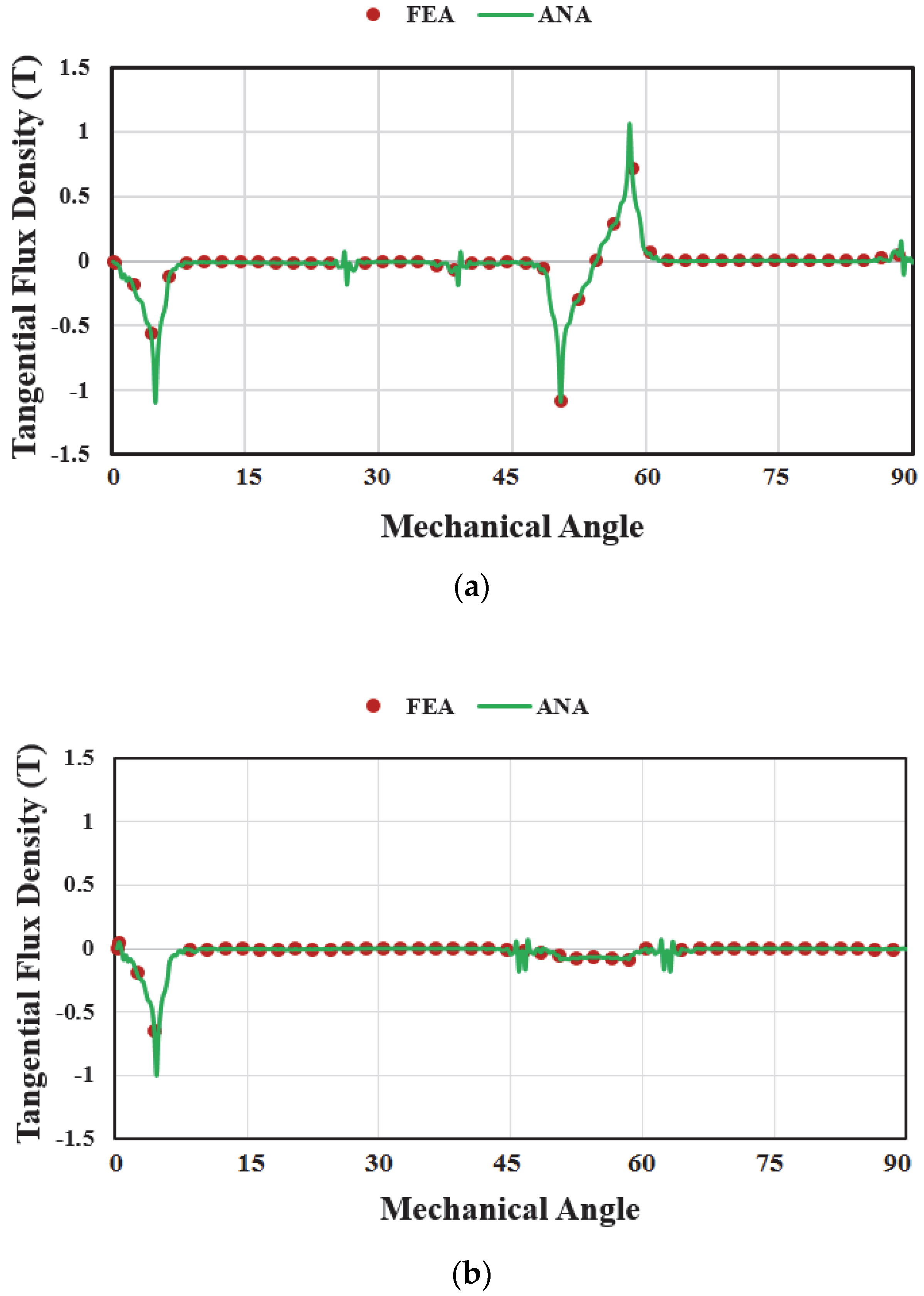
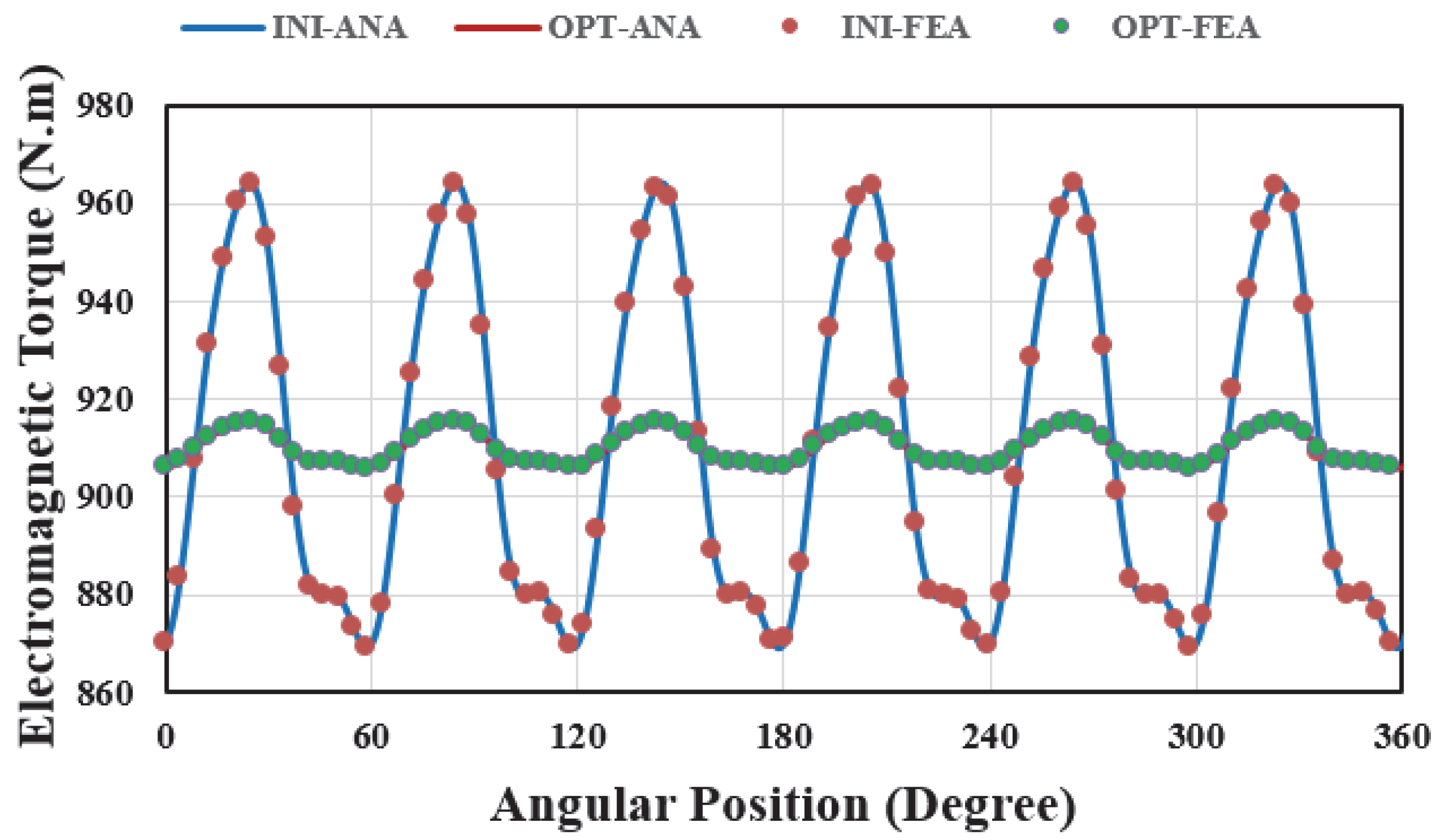
The 2D finite element method is applied to the performance calculation of the motor with uniform and non-uniform rotor shapes. The magnetic field distribution in the studied motors is represented in Figure 5. Open circuit analytical and numerical comparisons of the cogging torque for both motors with initial and optimal magnet shapes are shown in Figure 6. The on-load comparison of the back electromotive force of the investigate motors with the initial and optimal magnet shapes is carried out analytically and numerically as shown in Figure 7. An analytical and numerical comparison of the radial flux density for the 12S-10P motor in an open circuit and on-load condition is shown in Figure 8. An analytical and numerical comparison of tangential flux density for the 12S-10P motor in open circuit and on-load condition is shown in Figure 9. An on-load comparison of the electromagnetic torque of the 12S-10P motor with the initial and optimal magnet shapes is shown in Figure 10.
7. Conclusions
A mathematical expression for the optimal magnet shape in surface mounted permanent magnet machines was considered in this paper. The Fourier analysis method based on the subdomain method using hyperbolic functions is applied to derive the analytical expressions for the calculation of magnetic vector potential, magnetic flux density, cogging torque, electromagnetic torque and back-electromotive force in surface-mounted permanent magnet machines. This model is applied for the performance computation of a 12S-10P surface-mounted permanent magnet motor. The results of the proposed model have been verified thanks to the FEA results. In future work, the iron permeability for global saturation can be considered in the analytical model by Dubas’ superposition technique [35,36].
Conflicts of Interest
The author declares no conflict of interest.
References
- Jahns, T.M.; Soong, W.L. Pulsating torque minimization techniques for permanent magnet AC motor drives—A review. IEEE Trans. Ind. Electron. 1996, 43, 321–330. [Google Scholar] [CrossRef]
- Bianchi, N.; Bolognani, S. Design techniques for reducing the cogging torque in surface-mounted PM motors. IEEE Trans. Ind. Appl. 2002, 38, 1259–1265. [Google Scholar] [CrossRef]
- Lukaniszyn, M.; Jagiela, M.; Wrobel, R. Optimization of permanent magnet shape for minimum cogging torque using a genetic algorithm. IEEE Trans. Magn. 2004, 40, 1228–1231. [Google Scholar] [CrossRef]
- Lateb, R.; Takorabet, N.; Meibody-Tabar, F. Effect of magnet segmentation on the cogging torque in surface-mounted permanent-magnet motors. IEEE Trans. Magn. 2006, 42, 442–445. [Google Scholar] [CrossRef]
- Ackermann, B.; Sottek, R.; Janssen, J.H.H.; van Steen, R.I. New technique for reducing cogging torque in a class of brushless DC motors. IEE Proc. B Electric Power Appl. 1992, 139, 315–320. [Google Scholar] [CrossRef]
- Ishikawa, T.; Slemon, G.R. A method of reducing ripple torque in permanent magnet motors without skewing. IEEE Trans. Magn. 1993, 29, 2028–2031. [Google Scholar] [CrossRef]
- Keyhani, C.B.; Studer, T.; Sebastian, S.K.; Murthy, A. Study of cogging torque in permanent magnet machines. Electric Mach. Power Syst. 1999, 27, 665–678. [Google Scholar] [CrossRef]
- Li, T.; Slemon, G. Reduction of cogging torque in permanent magnet motors. IEEE Trans. Magn. 1988, 24, 2901–2903. [Google Scholar]
- Hwang, C.C.; John, S.B.; Wu, S.S. Reduction of cogging torque in spindle motors for CD-ROM drive. IEEE Trans. Magn. 1998, 34, 468–470. [Google Scholar] [CrossRef]
- Jabbari, A.; Shakeri, M.; Nabavi Niaki, S.A. Pole shape optimization of permanent magnet synchronous motors using the reduced basis technique. Iran. J. Electr. Electron. Eng. 2010, 6, 48–55. [Google Scholar]
- Markovic, M.; Jufer, M.; Perriard, Y. Reducing the cogging torque in brushless DC motors by using conformal mappings. IEEE Trans. Magn. 2004, 40, 451–455. [Google Scholar] [CrossRef]
- Zarko, D.; Ban, D.; Lipo, T.A. Analytical calculation of magnetic field distribution in the slotted air gap of a surface permanent-magnet motor using complex relative air-gap permeance. IEEE Trans. Magn. 2006, 42, 1828–1837. [Google Scholar] [CrossRef]
- Boughrara, K.; Zarko, D.; Ibtiouen, R.; Touhami, O.; Rezzoug, A. Magnetic field analysis of inset and surface-mounted permanent-magnet synchronous motors using Schwarz–Christoffel transformation. IEEE Trans. Magn. 2009, 45, 3166–3178. [Google Scholar] [CrossRef]
- Ilhan, E.; Gysen, B.L.J.; Paulides, J.J.H.; Lomonova, E.A. Analytical hybrid model for flux switching permanent magnet machines. IEEE Trans. Magn. 2010, 46, 1762–1765. [Google Scholar] [CrossRef]
- Tang, Y.; Motoasca, T.E.; Paulides, J.J.H.; Lomonova, E.A. Analytical modeling of flux-switching machines using variable global reluctance networks. In Proceedings of the 2012 XXth International Conference on Electrical Machines, Marseille, France, 2–5 September 2012; pp. 2792–2798. [Google Scholar]
- Hua, W.; Zhang, G.; Cheng, M.; Dong, J. Electromagnetic performance analysis of hybrid-excited flux-switching machines by a nonlinear magnetic network model. IEEE Trans. Magn. 2011, 47, 3216–3219. [Google Scholar] [CrossRef]
- Gu, Q.; Gao, H. Effect of slotting in PM electric machines. Electric Mach. Power Syst. 1985, 10, 273–284. [Google Scholar]
- Boules, N. Prediction of no-load flux density distribution in permanent magnet machines. IEEE Trans. Ind. Appl. 1985, 3, 633–643. [Google Scholar] [CrossRef]
- Ackermann, B.; Sottek, R. Analytical modeling of the cogging torque in permanent magnet motors. Electr. Eng. Archiv fur Elektrotechnik 1995, 78, 117–125. [Google Scholar] [CrossRef]
- Radun, A. Analytical calculation of the switched reluctance motor’s unaligned inductance. IEEE Trans. Magn. 1999, 35, 4473–4481. [Google Scholar] [CrossRef]
- Rasmussen, K.F.; Davies, J.H.; Miller, T.J.E.; McGelp, M.I.; Olaru, M. Analytical and numerical computation of air-gap magnetic fields in brushless motors with surface permanent magnets. IEEE Trans. Ind. Appl. 2000, 36, 1547–1554. [Google Scholar] [Green Version]
- Wang, X.; Li, Q.; Wang, S.; Li, Q. Analytical calculation of air-gap magnetic field distribution and instantaneous characteristics of brushless DC motors. IEEE Trans. Energy Convers. 2003, 18, 424–432. [Google Scholar] [CrossRef]
- Liu, Z.J.; Li, J.T. Analytical solution of air-gap field in permanent-magnet motors taking into account the effect of pole transition over slots. IEEE Trans. Magn. 2007, 43, 3872–3883. [Google Scholar] [CrossRef]
- Liu, Z.J.; Li, J.T.; Jiang, Q. An improved analytical solution for predicting magnetic forces in permanent magnet motors. J. Appl. Phys. 2008, 103, 07F135. [Google Scholar] [CrossRef]
- Liu, Z.J.; Li, J.T. Accurate prediction of magnetic field and magnetic forces in permanent magnet motors using an analytical solution. IEEE Trans. Energy Convers. 2008, 23, 717–726. [Google Scholar] [CrossRef]
- Kumar, P.; Bauer, P. Improved analytical model of a permanent-magnet brushless DC motor. IEEE Trans. Magn. 2008, 44, 2299–2309. [Google Scholar] [CrossRef]
- Lubin, T.; Mezani, S.; Rezzoug, A. Exact analytical method for magnetic field computation in the air gap of cylindrical electrical machines considering slotting effects. IEEE Trans. Magn. 2010, 46, 1092–1099. [Google Scholar] [CrossRef]
- Gysen, B.L.; Ilhan, E.; Meessen, K.J.; Paulides, J.J.; Lomonova, E.A. Modeling of flux switching permanent magnet machines with fourier analysis. IEEE Trans. Magn. 2010, 46, 1499–1502. [Google Scholar] [CrossRef]
- Boughrara, K.; Ibtiouen, R.; Lubin, T. Analytical prediction of magnetic field in parallel double excitation and spoke-type permanent-magnet machines accounting for tooth-tips and shape of polar pieces. IEEE Trans. Magn. 2012, 48, 2121–2137. [Google Scholar] [CrossRef]
- Boughrara, K.; Lubin, T.; Ibtiouen, R. General subdomain model for predicting magnetic field in internal and external rotor multiphase flux-switching machines topologies. IEEE Trans. Magn. 2013, 49, 5310–5325. [Google Scholar] [CrossRef]
- Tiang, T.L.; Ishak, D.; Jamil, M.K.M. Complete subdomain model for surface-mounted permanent magnet machines. In Proceedings of the 2014 IEEE Conference on Energy Conversion, Johor Bahru, Malaysia, 11–13 October 2014; pp. 140–145. [Google Scholar]
- Liu, X.; Hu, H.; Zhao, J.; Belahcen, A.; Tang, L.; Yang, L. Analytical solution of the magnetic field and EMF calculation in ironless BLDC motor. IEEE Trans. Magn. 2016, 52, 1–10. [Google Scholar] [CrossRef]
- Dubas, F.; Espanet, C. Analytical solution of the magnetic field in permanent-magnet motors taking into account slotting effect: No-load vector potential and flux density calculation. IEEE Trans. Magn. 2009, 45, 2097. [Google Scholar] [CrossRef]
- Roubache, L.; Boughrara, K.; Dubas, F.; Ibtiouen, R. New subdomain technique for electromagnetic performances calculation in radial-flux electrical machines considering finite soft-magnetic material permeability. IEEE Trans. Magn. 2018. [Google Scholar] [CrossRef]
- Dubas, F.; Boughrara, K. New scientific contribution on the 2-D subdomain technique in Cartesian coordinates: Taking into account of iron parts. Math. Comput. Appl. 2017, 22, 17. [Google Scholar]
- Dubas, F.; Boughrara, K. New scientific contribution on the 2-D subdomain technique in polar coordinates: Taking into account of iron parts. Math. Comput. Appl. 2017, 22, 42. [Google Scholar]
- Hannon, B.; Sergeant, P.; Dupré, L. Two-dimensional Fourier-based modeling of electric machines. In Proceedings of the 2017 IEEE International Electric Machines and Drives Conference, Miami, FL, USA, 21–24 May 2017; pp. 1–8. [Google Scholar]
- Jabbari, A. 2D Analytical Modeling of Magnetic Vector Potential in Surface Mounted and Surface Inset Permanent Magnet Machines. Iran. J. Electr. Electron. Eng. 2017, 13, 362–373. [Google Scholar]
- Jabbari, A. Exact analytical modeling of magnetic vector potential in surface inset permanent magnet DC machines considering magnet segmentation. J. Electr. Eng. 2018, 69, 39–45. [Google Scholar] [CrossRef] [Green Version]
- Jabbari, A. Analytical Modeling of Magnetic Field Distribution in Inner Rotor Brushless Magnet Segmented Surface Inset Permanent Magnet Machines. Iran. J. Electr. Electron. Eng. 2018, 14, 259–269. [Google Scholar]
- Jabbari, A. Analytical Modeling of Magnetic Field Distribution in Multiphase H-Type Stator Core Permanent Magnet Flux Switching Machines. Iran. J. Sci. Tech. Trans. Electr. Eng. 2018, 3, 1–13. [Google Scholar] [CrossRef]
Figure 1.
The geometrical representation of the investigated machines with (a) uniform rotor shape, (b) non-uniform rotor shape.
Figure 1.
The geometrical representation of the investigated machines with (a) uniform rotor shape, (b) non-uniform rotor shape.

Figure 2.
The stator subdomains including the and regions.

Figure 3.
The rotor permanent magnet subdomain. (a) Uniform rotor, (b) non-uniform rotor.

Figure 4.
The cross-sections of the studied motor. (a) with the uniform rotor; (b) uniform rotor, (c) with the optimal rotor, (d) optimal rotor.
Figure 4.
The cross-sections of the studied motor. (a) with the uniform rotor; (b) uniform rotor, (c) with the optimal rotor, (d) optimal rotor.

Figure 5.
The magnetic field distribution in the 12S-10P motor. (a) Initial magnet shape; (b) Optimal magnet shape.
Figure 5.
The magnetic field distribution in the 12S-10P motor. (a) Initial magnet shape; (b) Optimal magnet shape.

Figure 6.
An open circuit analytical and numerical comparison of the cogging torque.

Figure 7.
An on-load analytical and numerical comparison of Back-EMF.

Figure 8.
An analytical and numerical comparison of radial flux density for the 12S-10P motor. (a) Open circuit condition; (b) On-load condition.
Figure 8.
An analytical and numerical comparison of radial flux density for the 12S-10P motor. (a) Open circuit condition; (b) On-load condition.

Figure 9.
An analytical and numerical comparison of the tangential flux density for the 12S-10P motor. (a) Open circuit condition; (b) On-load condition.
Figure 9.
An analytical and numerical comparison of the tangential flux density for the 12S-10P motor. (a) Open circuit condition; (b) On-load condition.

Figure 10.
An on-load analytical and numerical comparison of the electromagnetic torque for the 12S-10P motor.
Figure 10.
An on-load analytical and numerical comparison of the electromagnetic torque for the 12S-10P motor.


Table 1.
The specification of the investigated motors.
| Parameter | Value |
|---|---|
| Rotor Outer Diameter | 208 mm |
| Rotor Inner Diameter | 130 mm |
| Number of poles | 10 |
| Pole Arc | 35° |
| Pole Thickness | 20 mm |
| Magnet material | NEO-39SH |
| Stator Outer Diameter | 350 mm |
| Stator Inner Diameter | 210 mm |
| Number of Slots | 12 |
| Stator Tooth Width | 30 mm |
| Stator Yoke Width | 26 mm |
| Slot Open | 7 mm |
| Tip Thickness | 2.5 mm |
| Slot Skew | 0° |
| Stator Length | 100 mm |
| Lamination material | M 19–0.5 mm |
© 2018 by the author. Licensee MDPI, Basel, Switzerland. This article is an open access article distributed under the terms and conditions of the Creative Commons Attribution (CC BY) license (http://creativecommons.org/licenses/by/4.0/).
Share and Cite
MDPI and ACS Style
Jabbari, A. An Analytical Expression for Magnet Shape Optimization in Surface-Mounted Permanent Magnet Machines. Math. Comput. Appl. 2018, 23, 57. https://0-doi-org.brum.beds.ac.uk/10.3390/mca23040057
AMA Style
Jabbari A. An Analytical Expression for Magnet Shape Optimization in Surface-Mounted Permanent Magnet Machines. Mathematical and Computational Applications. 2018; 23(4):57. https://0-doi-org.brum.beds.ac.uk/10.3390/mca23040057
Chicago/Turabian StyleJabbari, Ali. 2018. "An Analytical Expression for Magnet Shape Optimization in Surface-Mounted Permanent Magnet Machines" Mathematical and Computational Applications 23, no. 4: 57. https://0-doi-org.brum.beds.ac.uk/10.3390/mca23040057