High-Order Methods Applied to Nonlinear Magnetostatic Problems

Abstract

This paper presents a comparison between two high-order modeling methods for solving magnetostatic problems under magnetic saturation, focused on the extraction of machine parameters. Two formulations are compared, the first is based on the Newton-Raphson approach, and the second successively iterates the local remanent magnetization and the incremental reluctivity of the nonlinear soft-magnetic material. The latter approach is more robust than the Newton-Raphson method, and uncovers useful properties for the fast and accurate calculation of incremental inductance. A novel estimate for the incremental inductance relying on a single additional computation is proposed to avoid multiple nonlinear simulations which are traditionally operated with finite difference linearization or spline interpolation techniques. Fast convergence and high accuracy of the presented methods are demonstrated for the force calculation, which demonstrates their applicability for the design and analysis of electromagnetic devices.

1. Introduction

Electrical machine design often aims at achieving the highest power density, as it leads to weight and cost savings. High power density can be reached by different means, such as using efficient cooling methods [1] or by considering permanent magnets and slotted iron structures, where the latter benefits from a high magnetic permeability, and hence, a higher magnetic field within the same volume. However, the $BH$-characteristics of soft-magnetic materials exhibit strong nonlinearity when exposed to high field strengths which are necessary to reach increased power density. Motor topologies in current research, such as reluctance [2,3,4] or flux-switching machines [5], entirely rely on these phenomena. It is, therefore, of high importance to be able to rigorously calculate global electromagnetic quantities, such as forces and inductances, in presence of nonlinear material characteristics, as well as obtaining accurate local field distribution. Although local effects might not impair the global machine parameters calculation, it can affect the outcome of shape [6,7] and topology [8] optimizations. The attempts in improving the computational efficiency of the aforementioned machine design have focused the research on fast semi-analytical modeling techniques [9], and towards numerical methods ever more accurate. The high-order methods, which exploit higher-order elements, allow the increase of the degree of smoothness of the solution. Consequently, a faster convergence is achieved resulting in fewer degrees of freedom (dof) for the same error compared to low-order methods such as the Finite Elements Method (FEM). Recently, two high-order methods have gained attention namely, the Spectral Element Method (SEM) and Isogeometric Analysis (IGA) [10,11]. They are applied to modeling of magnetic devices such as actuators and electrical machines in [12,13,14,15].

In this paper, the high-order methods are applied to the modeling of magnetostatic problems under magnetic saturation. Although the implementation is addressed to isotropic and non-hysteretic properties for soft-magnetic materials, more complex material models can be included [16]. Two iterative approaches are considered to build the nonlinear material solvers. The first is based on the Newton-Raphson (NR) approach, and the second linearizes the model at each iteration with the help of an incremental reluctivity and remanence of the iron. The second approach allows the accurate estimation of the incremental inductance using a unique additional static computation. The nonlinear magnetostatic distributions of both high-order modeling methods are compared to the results obtained with standard magnetostatic simulation in FEM. Smoother results are obtained from the novel incremental inductance estimate, and faster convergence, i.e., higher accuracy per dof, is verified for the force computation. The post-processing routines, the fast convergence and excellent accuracy of SEM and IGA methods, are demonstrated on simple benchmarks, although these general results are applicable to any electrical machine geometry without shape limitation, in magnetostatic regime under saturation.

2. Modeling Methods

The presented work uses three different modeling methods for field computation applied to electrical machine analysis in which nonlinear isotropic iron is considered. Although they share the same Galerkin formulation [10], each of these methods uses different basis functions, quadrature rules, and space discretization techniques, which are briefly defined in the next section. A convergence analysis for different hp-refinements is performed, from which the reference space discretization is chosen for each modeling technique, and used for further comparison.

2.1. Finite Element Method

The Finite Element Method is the most popular and established method for solving a wide variety of problems described by partial differential equations. The results presented in this paper are based on the commercial software Altair/Flux2D [17]. It uses a space discretization based on triangular or quadrilateral meshes. First and second-order elements allow the expression of the problem in a large but sparse matrix and to obtain a relatively fast solution in 2D. The solution obtained by means of FEM is known to be very dependent on the mesh refinement, requiring both time and experience. Additionally, a curved geometry is approximated by linear or quadratic elements which influence the solution accuracy or comes at the cost of a high number of mesh elements, or h-refinement. Several coarse meshes will be used for comparing convergences obtained with the higher-order methods with the same number of dof, while a much denser mesh will be used to generate the reference solution for this method. Higher-order methods aim at offering more geometrical flexibility for design compared to FEM, as well as demonstrating a faster convergence while maintaining an acceptable overall computational effort.

2.2. Spectral Element Method

In both high-order methods, the geometry is discretized into two dimensional (2D) conforming patches and continuity is imposed on their interfaces. In the first benchmark, introduced in Figure 3a, the C-core geometry is discretized in 40 patches, and p-refinement is used to increase the order of the basis functions up to the eleventh order. Each patch is mapped to a parent element, where calculations are conducted [18]. In the parent element ${[-1,1]}^2$, Legendre polynomials are used as basis functions, the Lagrangian interpolation polynomials are used to change the representation to a nodal form, and obtain the gradients on the grid. Corresponding nodes of the grid are the Lobatto-Gauss-Legendre (LGL) roots [10,19]. These nodes have the particularity to include end-points {−1, 1}, hence, the Gauss-Lobatto quadrature is applied for numerical integration. The order of the Legendre polynomials directly links to the number of nodes in each parametric direction of the element. Complex shapes can be modeled, notwithstanding proper mapping transformations and operators of the contravariant fluxes are found [10,20].

2.3. Isogeometric Analysis

Isogeometric Analysis (IGA) has introduced a new paradigm in employing the same basis functions to represent exactly complex geometrical shapes, compute and visualize the solution [21]. These basis functions are structured through a tensor-product of B-splines which is the same functional description used in CAD models, and therefore, motivates their use. The physical domain containing the geometry is mapped to a rectangular computational domain on which the basis functions and their gradients are known and where the integrals are calculated through numerical Gaussian quadrature [22]. Contrarily to the Gauss-Lobatto quadrature, the end-points are not present in the quadrature nodes. The set of basis functions, which is mapped onto the physical domain, can be enriched by means of hp-refinements. Essential boundary conditions are imposed through $L^2$ projection [11]. Mathematical derivations introducing the framework of IGA can be found in [23] and its application to electromagnetic problems with linear material characteristics have been discussed in [14].

3. Problem Formulation

The Galerkin method is used to pass from the strong form of the problem deriving from Maxwell’s and constitutive equations, to the variational formulation, which is implemented [10]. The general 2D magnetostatic problem formulation with linear material characteristics with respect to the nodal magnetic vector potential, A, is given as a set of linear equations in matrix form:

$$\begin{array}{cc}\hfill SA& =I_{\mathrm{rhs}},\hfill \end{array}$$

(1)

$$\begin{array}{cc}\hfill {A|}_{{\mathsf{\Gamma }}_D}& =0,\hfill \end{array}$$

(2)

$$\begin{array}{cc}\hfill \frac{\partial A}{\partial \mathbf{n}}{|}_{{\mathsf{\Gamma }}_N}& =0,\hfill \end{array}$$

(3)

where,

$$\begin{array}{cc}\hfill S_{i,j}& ={\int }_{\mathsf{\Omega }}\nu \left(\mathbf{x}\right)\mathrm{grad}{\omega }_j·\mathrm{grad}{\omega }_{i}d\mathbf{x},\hfill \end{array}$$

(4)

$$\begin{array}{cc}\hfill I_{\mathrm{coil},i}& ={\int }_{{\mathsf{\Omega }}_{\mathrm{coil}}}{J}_{\mathrm{coil}}{\omega }_{i}d\mathbf{x},\hfill \end{array}$$

(5)

$$\begin{array}{cc}\hfill I_{\mathrm{pm},i}& ={\int }_{{\mathsf{\Omega }}_{\mathrm{pm}}}\nu \left(\mathbf{x}\right)\mathbf{M}·\mathrm{curl}{\omega }_{i}d\mathbf{x},\hfill \end{array}$$

(6)

in which $\omega$ are the set of basis functions considered depending on the method used. The right-hand side, $I_{\mathrm{rhs}}$, sums the different sources contributions described in (5) and (6). In the 2D Cartesian formulation, A represents the z component of the magnetic vector potential at the nodes, which naturally satisfies the divergence-free property. The magnetic flux density derives from the curl of the potential such as

$$\begin{array}{c}\hfill \mathbf{B}=\mathrm{curl}A=\left(\begin{array}{c}{\nabla }_{y}A\\ -{\nabla }_{x}A\\ 0\end{array}\right).\end{array}$$

(7)

The relative reluctivity $\nu \left(\mathbf{x}\right)={\left({\mu }_0{\mu }_r\left(\mathbf{x}\right)\right)}^{-1}$ depends on the material defined for each patch. The imposed current density source $J_{\mathrm{coil}}$ is considered uniformly distributed in the conductor, which is valid for magnetostatic problems such as considered in this paper. Therefore, the skin and proximity effects are neglected. For a permanent magnet, the source is derived from the curl of the magnetization vector, which in most cases, is uniformly distributed such that $\left|\mathbf{M}\right|={\mu }_0^{-1}{B}_{\mathrm{rem}}$. As expressed in (6), the action of the curl operator is transferred to the basis functions $\mathit{\omega }$ in the spirit of the Galerkin procedure, i.e., by multiplying by the test functions, integrating by parts and using the Green formula. This general formulation can be used to describe the non-uniform magnetization arising from nonlinear soft-magnetic material characteristics as well.

3.1. Successive Iterations (SI)

Beyond a certain level of magnetic excitation, the soft-magnetic iron material saturates, which decreases the relative permeability. In the meantime, the magnetic moments in the iron align locally with the field excitation direction, which creates an overall non-uniform magnetization. This non-uniform magnetization in the iron can be captured with the help of the spline interpolant of the discrete $BH$ values of the material characteristic, such as the one shown in the Figure 1. The modulus of the flux density, $B_{\mathrm{mod}}$, is calculated at each node together with the incremental reluctivity $\nu (\mathbf{x},\mathbf{B})$ and the non-uniform magnetization vector

$${\mathbf{M}}_{\mathrm{iron}}(\mathbf{x},\mathbf{B})=\mathit{\alpha }{B}_r{\mu }_0^{-1},$$

(8)

where $B_r$ is the remanent flux density in the iron, which is zero in the linear region. A graphical representation of the algorithm is given on Figure 1. The parameter $\mathit{\alpha }=\mathbf{B}{B}_{\mathrm{mod}}^{-1}$ represents the directional cosines of the flux density vector and helps orienting the magnetic remanence of the iron. As a result, an iterative model is proposed, where the solution is used to calculate the magnetic flux density distribution B in the soft-magnetic regions followed by the magnetic remanence and incremental reluctivity. Finally, the stiffness matrix entry from (4) is modified in the soft-magnetic regions, and an additional magnetic source term is added to the right-hand side:

$$\begin{array}{cc}\hfill S_{i,j}& ={\int }_{{\mathsf{\Omega }}_{\mathrm{iron}}}\nu (\mathbf{x},\mathbf{B})\mathrm{grad}{\omega }_j·\mathrm{grad}{\omega }_{i}d\mathbf{x},\hfill \end{array}$$

(9)

$$\begin{array}{cc}\hfill I_{\mathrm{iron},i}& ={\int }_{{\mathsf{\Omega }}_{\mathrm{iron}}}\nu (\mathbf{x},\mathbf{B}){\mathbf{M}}_{\mathrm{iron}}(\mathbf{x},\mathbf{B})·\mathrm{curl}{\omega }_{i}d\mathbf{x}.\hfill \end{array}$$

(10)

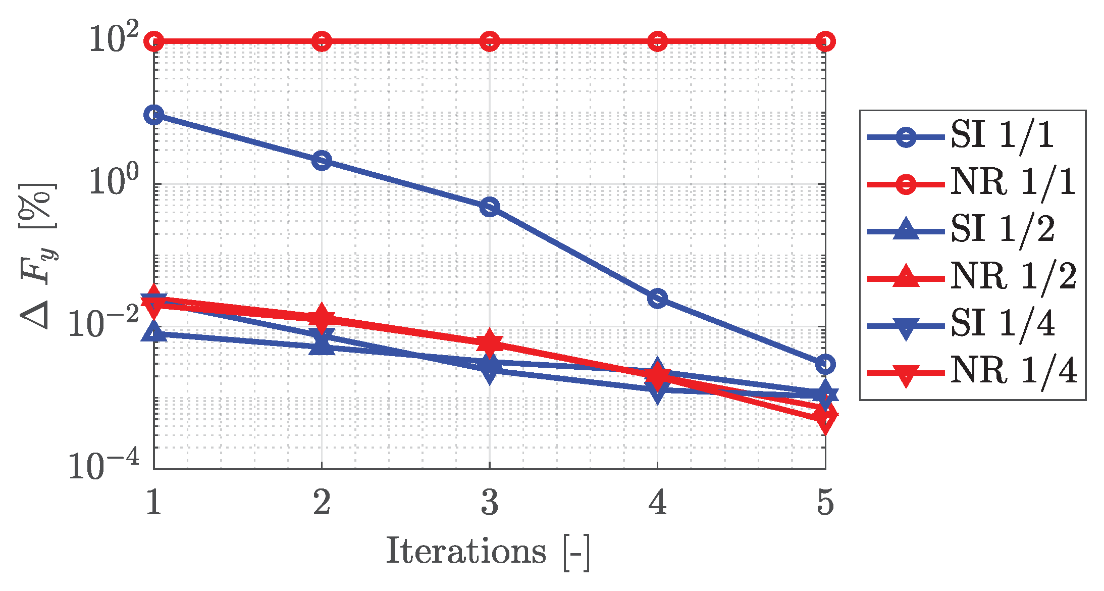
At each iteration, the solution vector is stored and the difference with the previous solution regarding the $L^2$ norm is calculated per patch. The maximum value is represented in the convergence comparison presented in Figure 2. The SI method presents some similarities with the locally convergent version of the fixed-point method discussed in [24,25]. The developed model is linearly convergent, robust, and contains a physical interpretation. Moreover, the non-uniform magnetic source term is useful to obtain additional parameters and insights of the electrical machine efficiently, such as the incremental inductance, which is detailed in section IV-B.

3.2. Newton-Raphson

A NR solver is considered to allow quadratic convergence to the solution. Such method is based on a first-order Taylor expansion of the residual which is to be minimized. The derivation details specific to a magnetic application can be found in [16]. The solution in the $n-$th iteration is approximated with a linearization $\mathrm{d}A$ and the solution A from the previous iteration:

$$A^n=A^{n-1}+\mathrm{d}{A}^{n-1},$$

(11)

where the increment $\mathrm{d}A$ is calculated as

$$J\mathrm{d}{A}^{n-1}=r.$$

(12)

Rewriting (1), the residual r is expressed as

$$r=I_{\mathrm{rhs}}-S_1\mathrm{d}{A}^{n-1}.$$

(13)

From (12), the Jacobian is defined as the derivative of the residual with respect to the solution vector

$$J={\displaystyle \frac{\partial r}{\partial A}}=S_1+S_2,$$

(14)

with

$$\begin{array}{cc}\hfill S_{1i,j}& ={\int }_{\mathsf{\Omega }}\nu (\mathbf{x},\mathbf{B})\mathrm{grad}{\omega }_j·\mathrm{grad}{\omega }_{i}d\mathbf{x},\hfill \end{array}$$

(15)

$$\begin{array}{cc}\hfill S_{2i,j}& ={\int }_{{\mathsf{\Omega }}_{\mathrm{iron}}}2\frac{\partial \nu (\mathbf{x},\mathbf{B})}{\partial B^2}\mathrm{grad}{\omega }_j·\mathbb{B}·\mathrm{grad}{\omega }_{i}d\mathbf{x},\hfill \end{array}$$

(16)

$$\begin{array}{cc}\hfill \mathbb{B}& =\left[\begin{array}{cc}{B}_y^2& -B_x{B}_y\\ -B_x{B}_y& B_x^2\end{array}\right].\hfill \end{array}$$

(17)

The NR method is implemented in the high-order method framework and the convergence is compared with the SI method in Figure 2. An important distinction between the SI and NR methods lies in the pre-processing of the $BH$-curve and the definition of the reluctivity $\nu (\mathbf{x},\mathbf{B})$:

$$\begin{array}{cc}\hfill \nu ={\nu }_{\mathrm{inc}}=\frac{\partial H}{\partial B},& \mathrm{with}\mathrm{SI},\hfill \end{array}$$

(18)

$$\begin{array}{cc}\hfill \nu ={\nu }_{\mathrm{app}}=\frac{H}{B},& \mathrm{with}\mathrm{NR}.\hfill \end{array}$$

(19)

Moreover, in the SI method, it may be necessary to ensure that the outputs of the algorithm are bounded by their physical limits with:

$$\begin{array}{c}\hfill {\nu }_r\in [{\nu }_{\mathrm{inc}}\left(0_{+}\right),1],\end{array}$$

(20)

$$\begin{array}{c}\hfill B_r\in [0,B_{\mathrm{sat}}],\end{array}$$

(21)

indeed, BH-curves may include an elbow within the very first data points which should not be considered. In the NR method, the $BH$-curve should be monotonic and may be linearly extended for higher values of the field. The NR method is especially valuable for time-domain problems [26], where the computational time becomes more critical. Additionally, to further enhance the convergence speed, relaxation methods [27,28] or hybrid methods [29] can be considered.

4. Post-Processing

In electrical machine design optimization, global quantities such as forces (attraction, propulsion, ripples) or inductances (self, mutual, magnetizing or incremental) are often present in the objective function or constraints. Therefore, it is important to ensure such quantities are computed both efficiently and accurately.

4.1. Force Calculation

In the FEM software, the electromechanical force is computed through the Virtual-Work (VW) method which relies on the differentiation of the magnetic co-energy $W_{\mathrm{m}}$ with respect to the displacement:

$$F_{\mathrm{VW}}=-\frac{\partial W_{\mathrm{m}}}{\partial \mathbf{x}},$$

(22)

$$W_{\mathrm{m}}={\int }_{\mathsf{\Omega }}d{W}_{\mathrm{m}}dV,$$

(23)

$$d{W}_{\mathrm{m}}={\int }_0^H\mathbf{B}\left(\mathbf{H}\right)d\mathbf{H}.$$

(24)

Because the $BH$-curve of the soft-magnetic material is nonlinear, this method tends to linearize this relation around the operating point. Its implementation is more cumbersome and requires the evaluation of volume integrals, using the nodal solution obtained iteratively. Additional evaluations are normally required to obtain the co-energy differentiation approximation around the operating point, although more efficient implementations have been proposed in [30,31].

Another method is the use of the Maxwell’s Stress Tensor (MST), $\mathbb{T}$, and is implemented for the considered high-order methods. By combining the Lorentz force equation, Ampere’s law and the Green-Ostrogradski theorem, the electromagnetic force can be written as:

$$F_{\mathrm{MST}}={\mu }_0^{-1}{\oint }_{\mathcal{S}}\mathbb{T}·\mathbf{n}dS,$$

(25)

$${\mathbb{T}}_{i,j}=(B_i{B}_j-\frac{1}{2}{\delta }_{i,j}{B}^2).$$

(26)

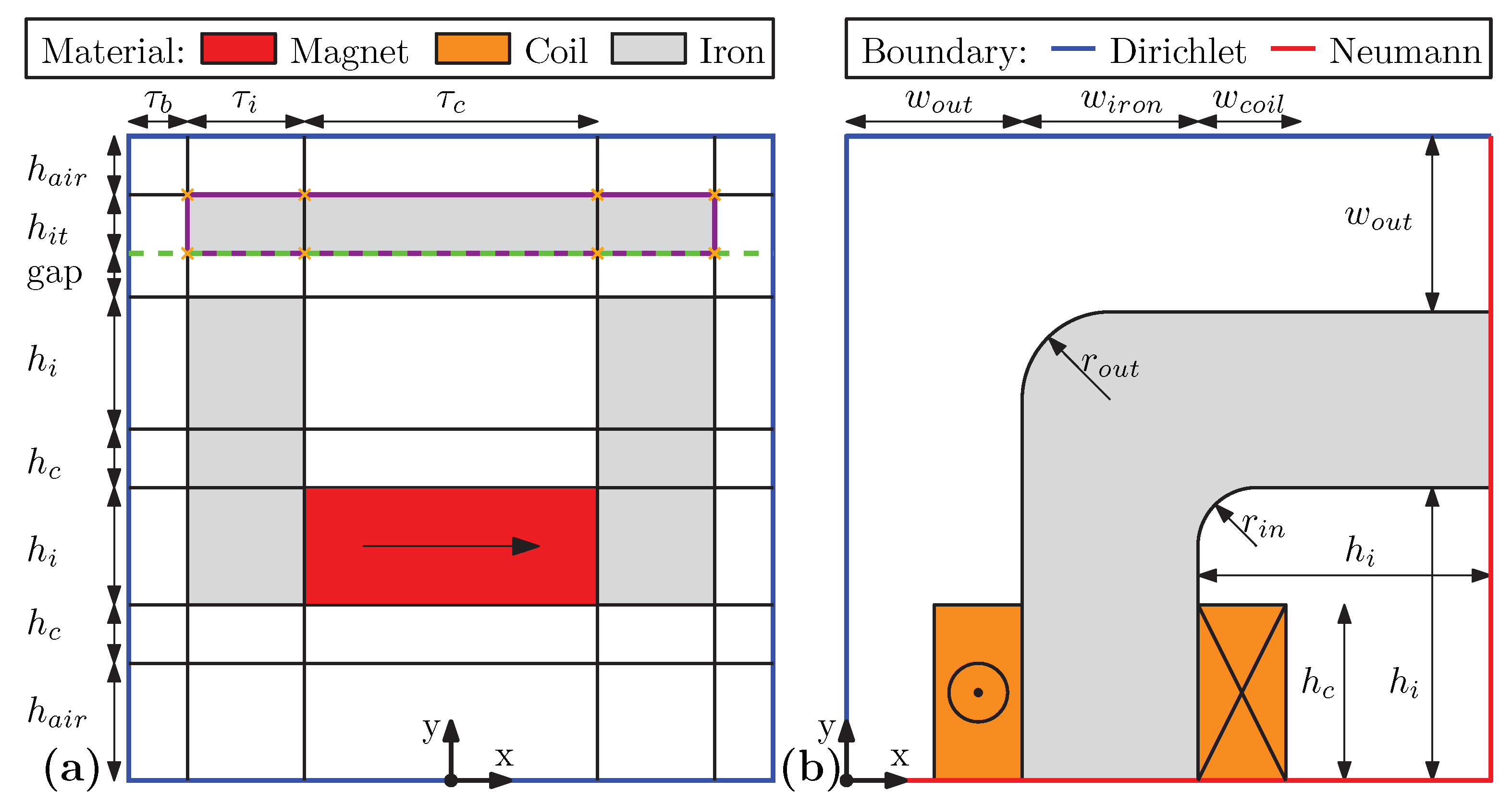
This formulation requires only one computation, and the numerical quadrature is reduced to an enclosing contour instead of all interior points, which reduces the computational load. It can be seen that some freedom exists in the choice of the enclosing contour. Hence, two integration paths are proposed, and can be seen in Figure 3a: the first path, pictured in magenta, takes the contour (CT) directly surrounding the solid of interest. The other path, in dashed green, only considers the top of the airgap (AG), because other lines lie on the Dirichlet boundary, where the solution and gradients vanish exactly.

4.2. Flux Linkage and Inductances Calculation

A direct evaluation of the magnetic vector potential in the coil region is used to obtain the flux linked by the coil, which is energized with a non-zero current source $I=J_{\mathrm{coil}}{S}_{\mathrm{coil}}=I_0$:

$$\begin{array}{cc}\hfill \varphi & =\frac{1}{S_{\mathrm{coil}}}{\int }_{V_{\mathrm{coil}}}A\left(\mathbf{x}\right)dV,I=I_0.\hfill \end{array}$$

(27)

While the apparent and incremental inductances are equal for linear materials, a distinction should be made in case of nonlinear iron characteristics.

$$L_{\mathrm{app}}=\frac{\varphi }{I_0},$$

(28)

$$L_{\mathrm{inc}}=\frac{\partial \varphi }{\partial I}\left(I_0\right).$$

(29)

Only the incremental inductance represents the saturation in the material and constitutes a useful parameter for order-reduction models [32], cross-coupling effects modeling and sensorless control [33]. When the magnetic circuit is energized by the $I_0$ current, a secondary magnetic source is induced in the nonlinear iron, as described in the SI method by Equation (10). Furthermore, by removing the current source, it is possible to compute the fluxes generated solely by the remanent magnetization in the iron:

$$\begin{array}{cc}\hfill {\varphi }_{\mathrm{rem}}& =\frac{1}{S_{\mathrm{coil}}}{\int }_{V_{\mathrm{coil}}}A\left(\mathbf{x}\right)dV,I=0.\hfill \end{array}$$

(30)

This method presents some analogies with the frozen permeability method which has been used in [34] for separating the different flux linkage contributions. Consequently, disregarding which of the SI or NR method is chosen, after the final iteration which determines $\varphi$, a unique simulation is needed to compute ${\varphi }_{rem}$ and therefore the proposed incremental inductance estimate can be calculated with:

$$\begin{array}{cc}\hfill L_{\mathrm{inc}}& =\frac{\varphi -{\varphi }_{\mathrm{rem}}}{I_0}.\hfill \end{array}$$

(31)

Indeed, the flux linkage characteristic is nonlinear with respect to current, similarly as the $BH$-curve, and the tangent of the flux linkage meets the intercept ${\varphi }_{\mathrm{rem}}$. On the contrary, in the FEM software, there is no direct option for the incremental inductance calculation. Therefore, to approach (29), a finite difference method must be considered which solves a two or three steps scenario and linearize the flux linkage around each operating current point $(\pm 1.0\times {10}^{-4}\mathrm{A})$. Such a method results in a parameter estimation which is less smooth and accurate, as well as more computationally cumbersome.

5. Results

Two different electromagnetic problems are simulated in SEM, IGA, and FEM. The topologies are presented in Figure 3, while the dimensions are summarized in

Table 1. Parameters for Benchmarks I and II.

Benchmark I Parameter	Value	Benchmark II Parameter	Value
${\tau }_c$	5 mm	$w_{iron}$	10 mm
${\tau }_i$	2 mm	$h_c$	10 mm
${\tau }_b$	5 mm	$w_{out}$	12 mm
$h_{air}$	5 mm	$r_{in}$	2 mm
$h_c$	2 mm	$r_{out}$	5 mm
$h_i$	3 mm	$w_{coil}$	5 mm
$h_{it}$	2 mm	$h_i$	18 mm
gap	1 mm

. Benchmark I is a C-core actuator, with straight corners, comporting a permanent magnet $(B_{\mathrm{rem}}=1.38\mathrm{T})$. Benchmark II is a quarter magnetic circuit of a transformer, with round edges.

5.1. Benchmark I

In Figure 4, different discretizations arising from p-refinements for SEM and hp-refinements for IGA are used to solve Benchmark I, with both SI and NR methods, and the attraction force $-F_y$ calculated with both integration contours (AG and CT) are given. It is interesting to note that the force obtained from both SI and NR methods have extremely close values, because the field distribution matches in the airgap and on the MST integration contour, although the field distribution differs locally in the iron, as seen on Figure 5. With IGA, different hp-refinements combinations can result in the same number of dof. For the range of dof considered in this paper, a mesh size subdivision of 4 per parametric direction offers the least sensitivity on the force calculation with respect to the order of the polynomial used. Therefore, the IGA reference discretization using $h=1/4$, $p=4$ and four Gauss points per direction and generating 2052 dof is chosen to compare the distribution of the magnetic vector potential in Figure 5 and Figure 6. The same number of dof is taken to generate the reference SEM discretization, which corresponds to $p=7$, and demonstrates good results as well. The mesh of FEM is still relatively coarse for this number of dof, therefore, a finer second-order mesh with 142841 nodes is generated to obtain the reference discretization results of

Table 2. Force comparison for Benchmark I reference solutions.

Method	Calculation	${\mathit{F}}_{\mathit{x}}$[N/mm]	${\mathit{F}}_{\mathit{y}}$[N/mm]
FEM	VW	$-1.774\times {10}^{-15}$	$-\mathbf{5.329}\times {10}^{-1}$
IGA	MST - CT	$-2.852\times {10}^{-15}$	$-5.288\times {10}^{-1}$
	MST - AG	$-3.578\times {10}^{-15}$	$-5.322\times {10}^{-1}$
SEM	MST - CT	$+3.018\times {10}^{-15}$	$-5.447\times {10}^{-1}$
	MST - AG	$+3.795\times {10}^{-15}$	$-5.318\times {10}^{-1}$
Difference	Regarding ${\mathit{F}}_{\mathit{y}}$ from	FEM(VW) [%]	IGA(AG) [%]
FEM	VW	-	0.157
IGA	MST - CT	0.780	0.624
	MST - AG	0.130	-
SEM	MST - CT	2.203	2.458
	MST - AG	0.213	0.036

, which demonstrate the slow convergence of FEM. Although not directly demonstrated in this paper, the convergence of the residual is faster for lower degrees of the basis functions. This might explain the slight advantage in terms of convergence speed for IGA over SEM in Figure 2. Moreover, although the convergence of the residual differs depending on the selected solver, the convergence of the force in the airgap shown on Figure 7, is similar between both solvers and requires around 5 iterations to be as close as ${10}^{-3}$% of the final value. It can be seen that on coarse grids without subdivision, i.e., $h=1/1$, the SI method is more robust than NR which fails to converge due to conditioning issues.

The values and differences of the attraction force $F_y$ for the reference solutions are gathered in Table 2. Good agreement can be seen between the high-order methods using the MST, and the VW calculation in FEM. Moreover, excellent agreement between SEM and IGA is obtained with airgap integration. The amplitude of the MST diverges at the geometric corners. As the integration is done per line, the airgap integration presents two singularities when the contour one exhibits eight in total, leading to some discrepancy, as shown on Figure 4. The airgap integration is favored, as numerical noise is minimized by taking advantage of having three contributions lying on Dirichlet boundaries, where the fields and their gradients vanish exactly. Finally, the numerical error of the contour integration is higher in SEM than in IGA since the corner points are included in the Gauss-Lobatto quadrature.

In Figure 6, the magnetic vector potential is shown for Benchmark I, as well as the absolute difference between FEM and both SEM and IGA solutions obtained with the reference discretizations. The solution obtained by FEM is expressed on a rectangular 2D grid for each patch. The same procedure is applied with the high-order methods, where the solution is interpolated on the common grid so that the solutions can be compared.

It is tedious to compare the computational effort as the methods are implemented on different platforms. The commercial FEM software is heavily optimized for solving big sparse linear systems. Moreover, its simulation time together with the meshing time is difficult to estimate. Otherwise, SEM and IGA, are implemented in MATLAB with different implementation strategies and no particular optimization of the code speed has been performed. Therefore, more research is necessary to improve the platforms and evaluate the computational load of the methods.

5.2. Benchmark II

For Benchmark II, the flux linkage is calculated for several currents and interpolated by splines, in the same way as the $BH$-curve. This interpolant is then differentiated with respect to the current and constitutes a smooth reference solution. The remanent flux linearization method introduced in this paper and calculated with Equation (31) perfectly evaluates the original differentiation of Equation (29). This novel method demonstrates a noticeable gain in both smoothness and accuracy compared to the finite difference approach used with FEM for the incremental inductance calculation, as shown in Figure 8. It should be noted that the incremental inductance computed from the remanent flux linearization is calculated independently from other current levels in the Figure 8. Therefore, for an accurate calculation of the incremental inductance for $I=10\mathrm{A}$, it is not necessary to calculate the apparent inductances for other current levels, as it is done in the case of finite difference or spline interpolation techniques. Instead the incremental inductance is computed from the remanent flux ${\varphi }_{\mathrm{rem}}$. Such accurate insights are beneficial in highly saturated machine control [35,36,37], and in field-weakening machine-based applications [34]. Moreover, the computational efficiency of this calculation makes it appealing in repetitive loops present in design optimization problems.

6. Conclusions

In this paper, two methods using high-order polynomials have been applied to the modeling and analysis of two benchmark problems with nonlinear material $BH$-curve. Calculation methods for extracting electrical machine characteristics in presence of nonlinear material, such as force, flux linkage and inductances have been discussed. The convergence of the force for different space discretizations has been shown. A convergence analysis of the residual of the solution obtained from two different formulations has been presented. SEM and IGA have demonstrated a higher accuracy per degree of freedom when compared to FEM which demonstrates the applicability of such methods for the design-through-analysis of electrical machines under magnetic saturation. Finally, a novel incremental inductance calculation technique has been proposed which increases the accuracy compared to existing methods while being computationally advantageous.

References

- Van Beek, T.A.; Jansen, J.W.; Gysen, B.L.J.; Lomonova, E.A. Comparison of direct and indirectly liquid-cooled coreless linear actuators with multi-layer coils. In Proceedings of the 11th International Symposium on Linear Drives for Industry Applications (LDIA), Osaka, Japan, 6–8 September 2017; pp. 1–6. [Google Scholar]
- Bao, J.; Gysen, B.L.J.; Boynov, K.; Paulides, J.J.H.; Lomonova, E.A. Torque Ripple Reduction for 12-Stator/10- Rotor-Pole Variable Flux Reluctance Machines by Rotor Skewing or Rotor Teeth Non-Uniformity. IEEE Trans. Magn. 2017, 53, 1–5. [Google Scholar] [CrossRef]
- Djelloul-Khedda, Z.; Boughrara, K.; Dubas, F.; Ibtiouen, R. Nonlinear Analytical Prediction of Magnetic Field and Electromagnetic Performances in Switched Reluctance Machines. IEEE Trans. Magn. 2017, 53, 1–11. [Google Scholar] [CrossRef]
- Mohammed, B.; Boughrara, K.; Dubas, F.; Ibtiouen, R. Two-Dimensional Exact Subdomain Technique of Switched Reluctance Machines with Sinusoidal Current Excitation. Math. Comput. Appl. 2018, 23, 59. [Google Scholar]
- Gysen, B.L.J.; Ilhan, E.; Meessen, K.J.; Paulides, J.J.H.; Lomonova, E.A. Modeling of flux switching permanent magnet machines with Fourier analysis. IEEE Trans. Magn. 2010, 46, 1499–1502. [Google Scholar] [CrossRef]
- Lee, S.; Lee, J.; Cho, S. Isogeometric Shape Optimization of Ferromagnetic Materials in Magnetic Actuators. IEEE Trans. Magn. 2016, 52, 1–8. [Google Scholar] [CrossRef]
- Dang Manh, N.; Evgrafov, A.; Gravesen, J.; Lahaye, D. Iso-geometric shape optimization of magnetic density separators. COMPEL Int. J. Comput. Math. Electr. Electron. Eng. 2014, 33, 1416–1433. [Google Scholar] [CrossRef]
- Gangl, P.; Amstutz, S.; Langer, U. Topology Optimization of Electric Motor Using Topological Derivative for Nonlinear Magnetostatics. IEEE Trans. Magn. 2016, 52, 1–4. [Google Scholar] [CrossRef]
- Ramakrishnan, K.; Curti, M.; Zarko, D.; Mastinu, G.; Paulides, J.J.H.; Lomonova, E.A. Comparative analysis of various methods for modelling surface permanent magnet machines. IET Electr. Power Appl. 2017, 11, 540–547. [Google Scholar] [CrossRef]
- Kopriva, D.A. Implementing Spectral Methods for Partial Differential Equations; Springer: Dordrecht, The Netherlands, 2009. [Google Scholar]
- Vázquez, R. A new design for the implementation of isogeometric analysis in Octave and Matlab: GeoPDEs 3.0. Comput. Math. Appl. 2016, 72, 523–554. [Google Scholar] [CrossRef]
- De Gersem, H. Coupled finite element - spectral element discretization for models with circular inclusions and far field domains. In Proceedings of the 4th International Conference on Computation in Electromagnetics, Bournemouth, UK, 8–11 April 2002; p. 27. [Google Scholar]
- Curti, M.; van Beek, T.A.; Jansen, J.W.; Gysen, B.L.J.; Lomonova, E.A. General Formulation of the Magnetostatic Field and Temperature Distribution in Electrical Machines Using Spectral Element Analysis. IEEE Trans. Magn. 2018, 54, 1–9. [Google Scholar] [CrossRef]
- Bontinck, Z.; Corno, J.; Gersem, H.D.; Kurz, S.; Pels, A.; Schöps, S.; Wolf, F.; de Falco, C.; Dölz, J.; Vázquez, R.; et al. Recent Advances of Isogeometric Analysis in Computational Electromagnetics. arXiv, 2017; arXiv:1709.06004. [Google Scholar]
- Mahariq, I. On the application of the spectral element method in electromagnetic problems involving domain decomposition. Turk. J. Electr. Eng. Comput. Sci. 2017, 25, 1059–1069. [Google Scholar] [CrossRef]
- Gyselinck, J.; Vandevelde, L.; Melkebeek, J.; Dular, P. Complementary two-dimensional finite element formulations with inclusion of a vectorized Jiles-Atherton model. COMPEL Int. J. Comput. Math. Electr. Electron. Eng. 2004, 23, 959–967. [Google Scholar] [CrossRef]
- Flux 12.2 User’s Guide. 2016. Available online: https://altairhyperworks.com/product/flux (accessed on 29 January 2019).
- Trefethen, L.N. Spectral Methods in MATLAB; Society for Industrial and Applied Mathematics: Philadelphia, PA, USA, 2000. [Google Scholar]
- Kopriva, D.A.; Gassner, G. On the quadrature and weak form choices in collocation type discontinuous Galerkin spectral element methods. J. Sci. Comput. 2010, 44, 136–155. [Google Scholar] [CrossRef]
- Curti, M.; Paulides, J.J.H.; Lomonova, E.A. Magnetic Modeling of a Linear Synchronous Machine with the Spectral Element Method. IEEE Trans. Magn. 2017, 53, 1–6. [Google Scholar] [CrossRef]
- Cottrell, J.A.; Hughes, T.J.; Bazilevs, Y. Isogeometric Analysis: Toward Integration of CAD and FEA; John Wiley & Sons: Hoboken, NJ, USA, 2009. [Google Scholar]
- Buffa, A.; Sangalli, G.; Vázquez, R. Isogeometric methods for computational electromagnetics: B-spline and T-spline discretizations. J. Comput. Phys. 2014, 257, 1291–1320. [Google Scholar] [CrossRef]
- Da Veiga, L.B.; Buffa, A.; Sangalli, G.; Vázquez, R. Mathematical analysis of variational isogeometric methods. Acta Numer. 2014, 23, 157–287. [Google Scholar] [CrossRef]
- Dlala, E.; Arkkio, A. Analysis of the Convergence of the Fixed-Point Method Used for Solving Nonlinear Rotational Magnetic Field Problems. IEEE Trans. Magn. 2008, 44, 473–478. [Google Scholar] [CrossRef]
- Dlala, E.; Arkkio, A. General formulation for the Newton-Raphson method and the fixed-point method in finite-element programs. In Proceedings of the XIX International Conference on Electrical Machines, Rome, Italy, 6–8 September 2010; pp. 1–5. [Google Scholar]
- Yan, S.; Jin, J.M.; Wang, C.F.; Kotulski, J.D. Numerical study of a time-domain finite element method for nonlinear magnetic problems in three dimensions. Prog. Electromagn. Res. 2015, 153, 69–91. [Google Scholar] [CrossRef]
- Fujiwara, K.; Okamoto, Y.; Kameari, A.; Ahagon, A. The Newton-Raphson method accelerated by using a line search—Comparison between energy functional and residual minimization. IEEE Trans. Magn. 2005, 41, 1724–1727. [Google Scholar] [CrossRef]
- Li, S.; Cui, X. An edge-based smoothed finite element method for nonlinear magnetostatic and eddy current analysis. Appl. Math. Model. 2018, 62, 287–302. [Google Scholar] [CrossRef]
- Vande Sande, H.; Boonen, T.; De Gersem, H.; Henrotte, F.; Hameyer, K. A hybrid Picard-Newton acceleration scheme for non-linear timeharmonic problems. In Proceedings of the 6th International Conference on Computational Electromagnetics, Aachen, Germany, 4–6 April 2006; pp. 1–2. [Google Scholar]
- Kim, D.H.; Lowther, D.A.; Sykulski, J.K. Efficient force calculations based on continuum sensitivity analysis. IEEE Trans. Magn. 2005, 41, 1404–1407. [Google Scholar]
- Kim, D.H.; Lowther, D.A.; Sykulski, J.K. Efficient Global and Local Force Calculations Based on Continuum Sensitivity Analysis. IEEE Trans. Magn. 2007, 43, 1177–1180. [Google Scholar] [CrossRef]
- Bottesi, O.; Alberti, L.; Sabariego, R.V.; Gyselinck, J. Finite element small-signal simulation of electromagnetic devices considering eddy currents in the laminations. IEEE Trans. Magn. 2017, 53, 1–8. [Google Scholar] [CrossRef]
- El-Murr, G.; Giaouris, D.; Finch, J.W. Online cross-coupling and self incremental inductances determination of salient permanent magnet synchronous machines. In Proceedings of the 5th IET International Conference on Power Electronics, Machines and Drives (PEMD 2010), Brighton, UK, 19–21 April 2010; pp. 1–4. [Google Scholar]
- Li, G.J.; Zhu, Z.Q.; Jewell, G. Performance investigation of hybrid excited switched flux permanent magnet machines using frozen permeability method. IET Electr. Power Appl. 2015, 9, 586–594. [Google Scholar] [CrossRef]
- Lin, Z.; Reay, D.; Williams, B.; He, X. High-performance current control for switched reluctance motors based on on-line estimated parameters. IET Electr. Power Appl. 2010, 4, 67–74. [Google Scholar] [CrossRef]
- Hemmati, S.; Kojoori, S.S.; Saied, S.; Lipo, T.A. Modelling and experimental validation of internal short-circuit fault in salient-pole synchronous machines using numerical gap function including stator and rotor core saturation. IET Electr. Power Appl. 2013, 7, 391–399. [Google Scholar] [CrossRef]
- Wang, L.; Aleksandrov, S.; Tang, Y.; Paulides, J.J.H.; Lomonova, E.A. Fault-tolerant electric drive and space-phasor modulation of flux-switching permanent magnet machine for aerospace application. IET Electr. Power Appl. 2017, 11, 1416–1423. [Google Scholar] [CrossRef]
Figure 1.
Graphical representation of the SI algorithm. Underlying -curve corresponds to the soft-magnetic material Cogent M800 50Hz 50A.
Figure 2.
Comparison of the convergence of the residual in Benchmark I.
Figure 3.
(a) Benchmark I: C-core permanent magnet actuator. (b) Benchmark II: Rounded-edge magnetic circuit quarter.
Figure 4.
Convergence of the attraction force for Benchmark I for different refinements.
Figure 5.
Differences in the magnetic vector potential distribution in [Vs/m] between (a) IGA(SI)-IGA(NR) and (b) SEM(SI)-SEM(NR) solutions, all using the reference discretizations.
Figure 6.
(a) Magnetic potential distribution in [Vs/m] and isolines obtained with IGA, (b–d), show the nodal differences between IGA-SEM, IGA-FEM, SEM-FEM reference solutions obtained with SI.
Figure 7.
Convergence of the attraction force regarding SI and NR solver iterations, for Benchmark I for different h-refinements, with in IGA.
Figure 8.
Apparent and incremental inductance comparison for Benchmark II.