Exact Two-Dimensional Analytical Calculations for Magnetic Field, Electromagnetic Torque, UMF, Back-EMF, and Inductance of Outer Rotor Surface Inset Permanent Magnet Machines


Abstract
:1. Introduction
2. Extracting the Magnetic Model
2.1. Assumptions
- (a)
- According to the geometry and the absence of skewing, the problem is solved in 2-D polar coordinates which means the end effect is neglected.
- (b)
- Magnetic vector potential has just axial component which is function of r and . Consequently, magnetic flux density has radial and tangential component; i.e., , .
- (c)
- All materials are isotropic.
- (d)
- Rotor and stator back iron have infinite permeability.
- (e)
- The edges of the slots and slot-openings have radial direction.
- (f)
- The eddy current effect is neglected.
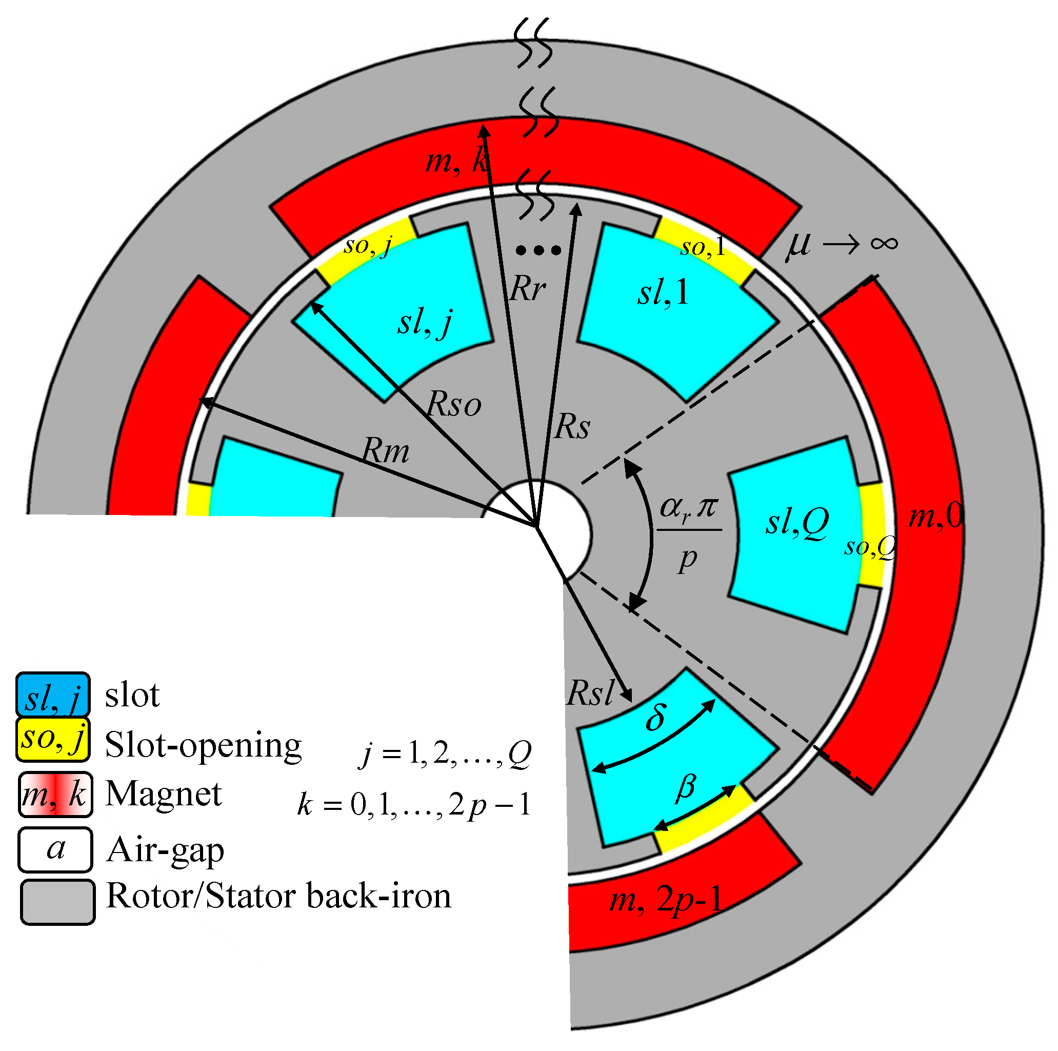
2.2. Dividing Region into Sub-Regions
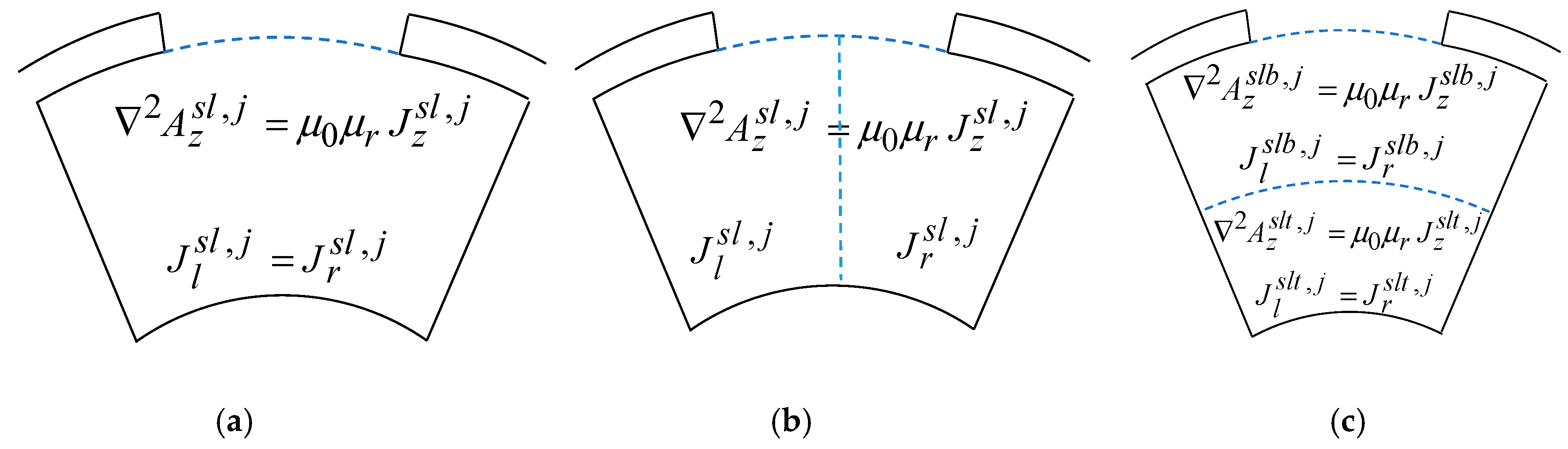
2.3. Extracting the Magnetic Model
2.4. Boundary Conditions
| Domain (i) | Domain (i+) | Equation | Border of the Interface | Limit | |
| Magnet | Rotor yoke | (15) | |||
| Magnet | Iron next to the PM pole | (16) | |||
| Air-gap | Magnet | (17) | |||
| Air-gap | Magnet | (18) | |||
| Slot-opening | Edges of slot-opening | (19) | |||
| Air-gap | Slot-opening | (20) | |||
| Air-gap | Slot-opening | (21) | |||
| Slot | Slot-opening | (22) | |||
| Slot | Edge of tooth Slot-opening Edge of tooth | (23) | |||
| Slot | Edges of the slot | (24) | |||
| Slot | Stator yoke | (25) |
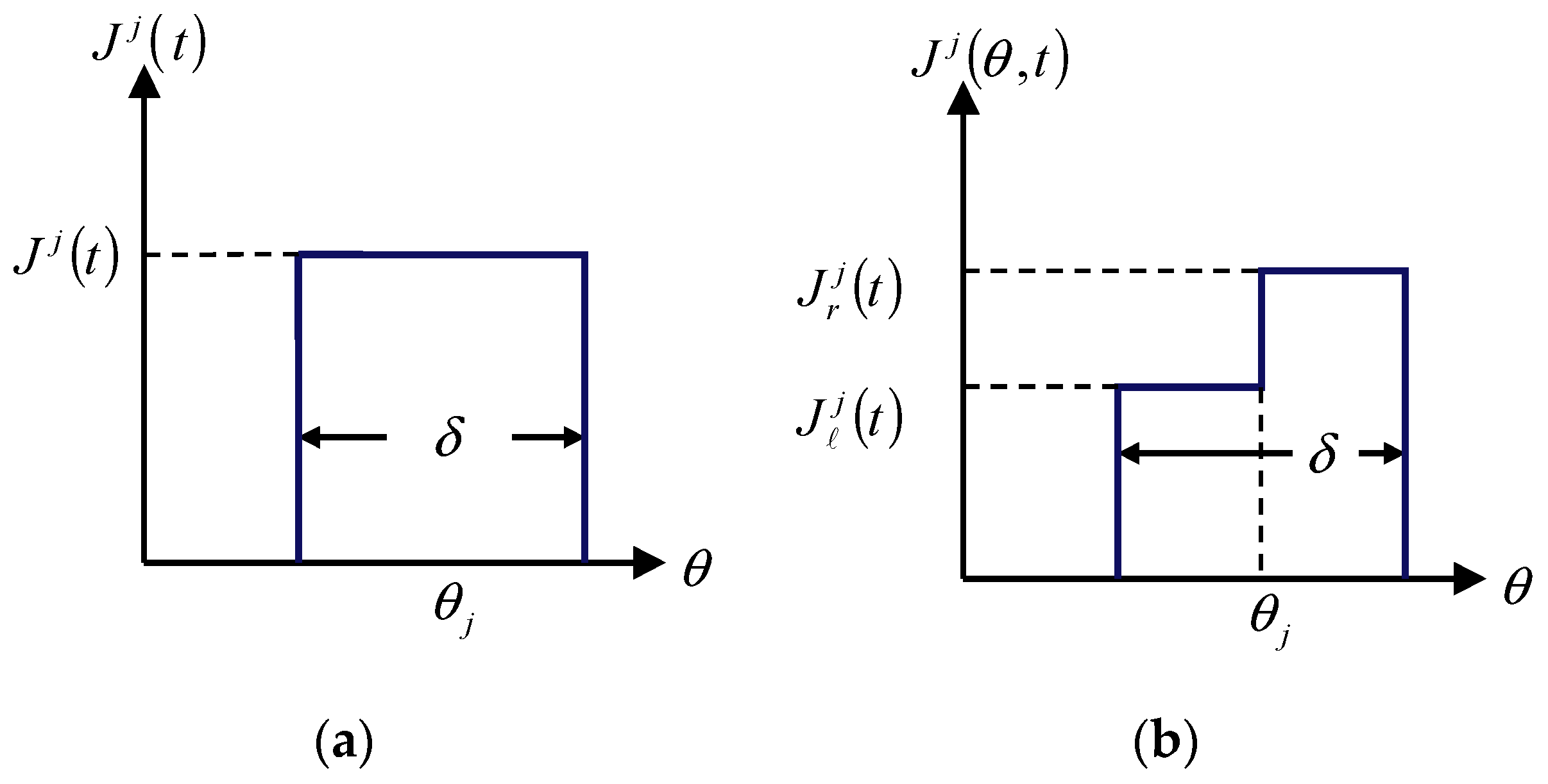
2.5. Extracting the Fourier Series of the Armature Reaction
2.6. Extracting the Fourier Series of the Magnetization
2.7. Finding the General Solution
2.8. Obtaining Integral Coefficients
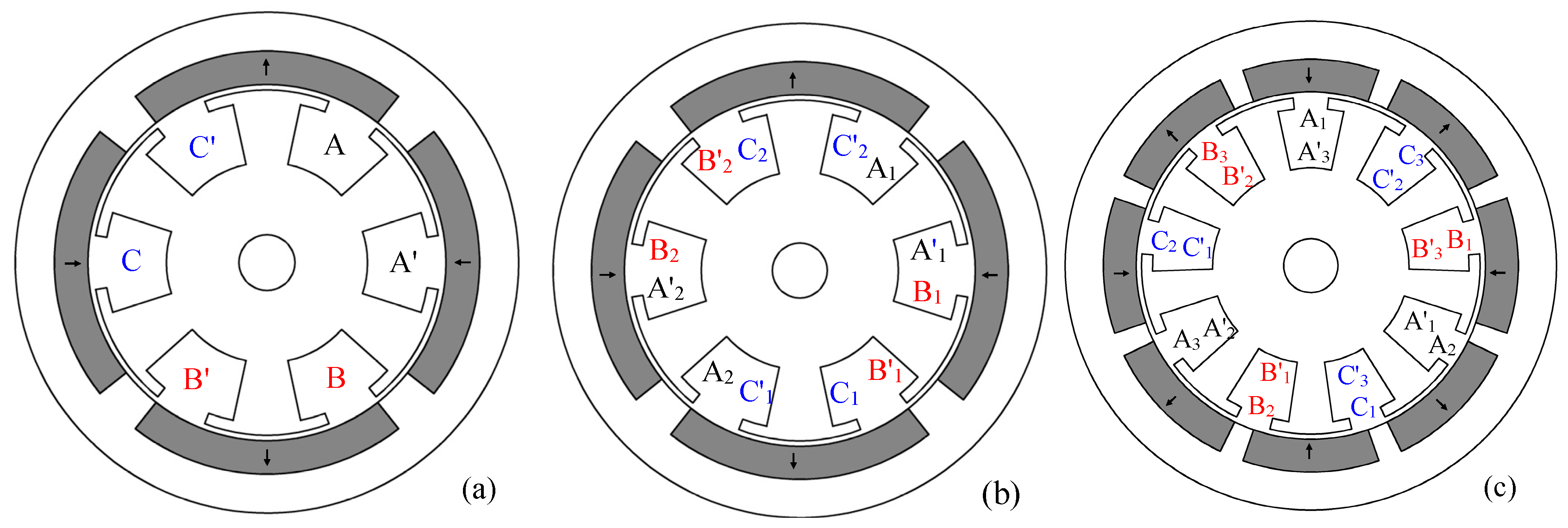
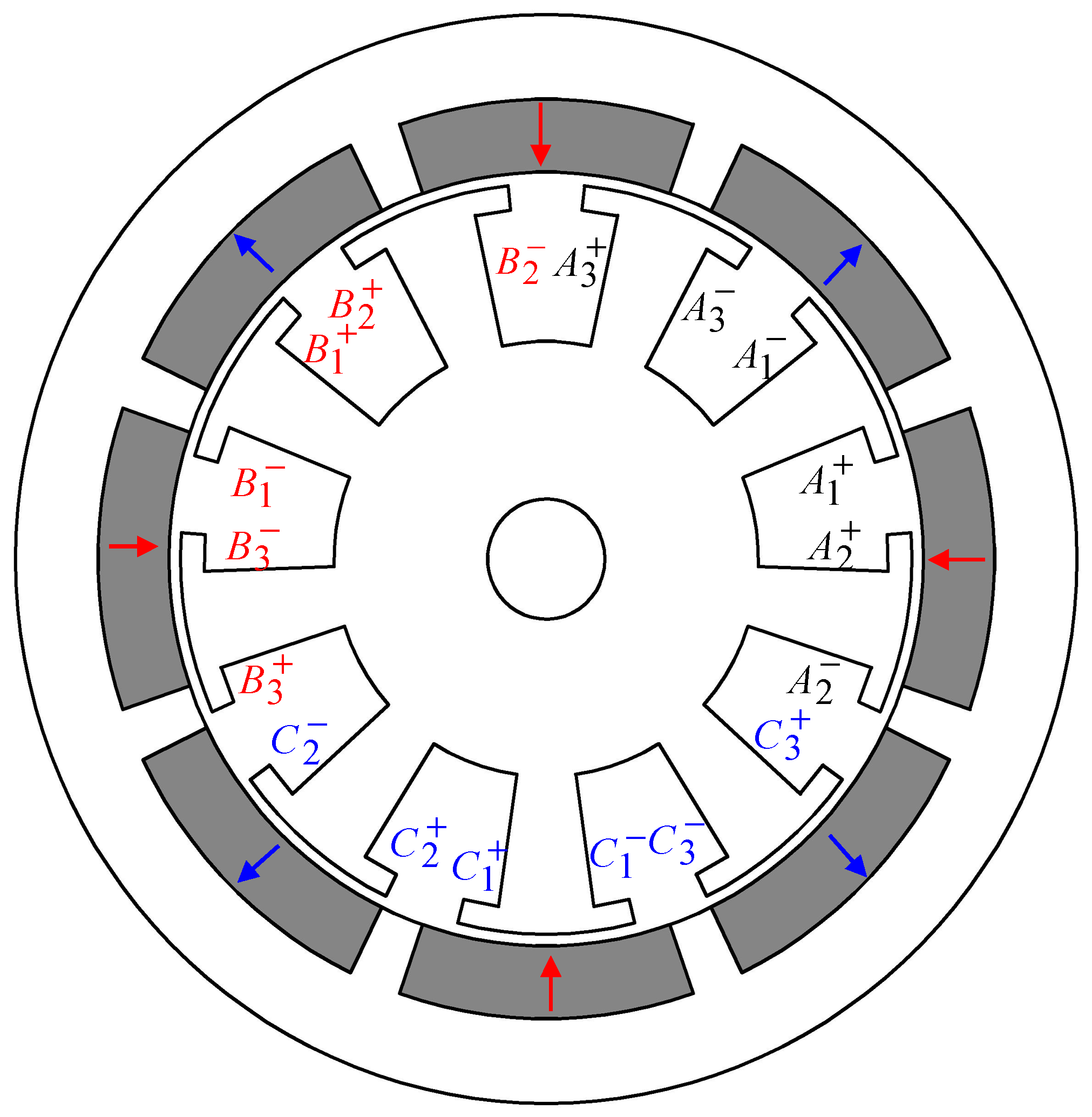
2.9. Overlapping Winding
3. Quantities
3.1. Flux Density
3.2. Inductances
3.3. Back-EMF
3.4. Instantaneous Electromagnetic Torque
3.5. Unbalanced Magnetic Force
4. Results
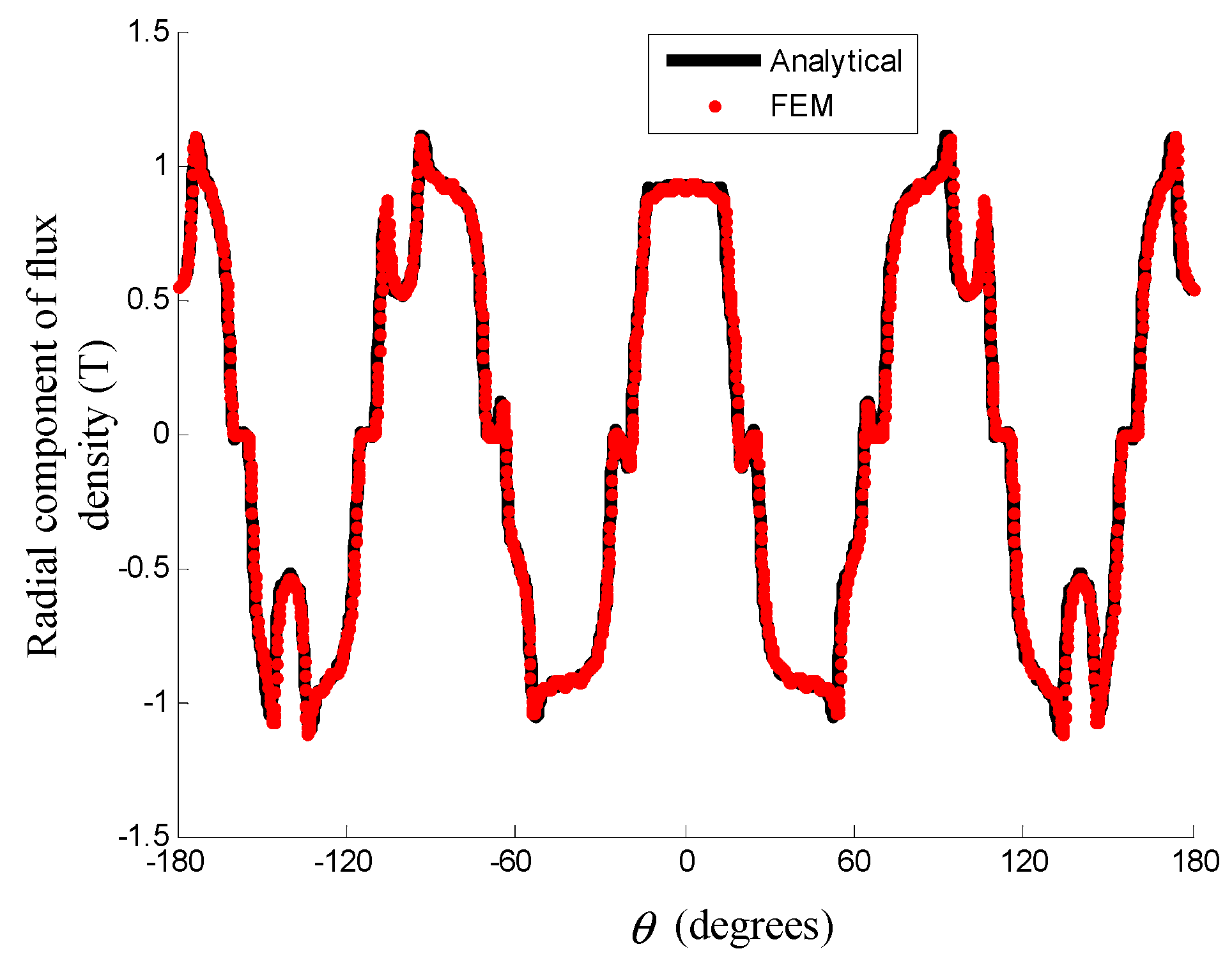
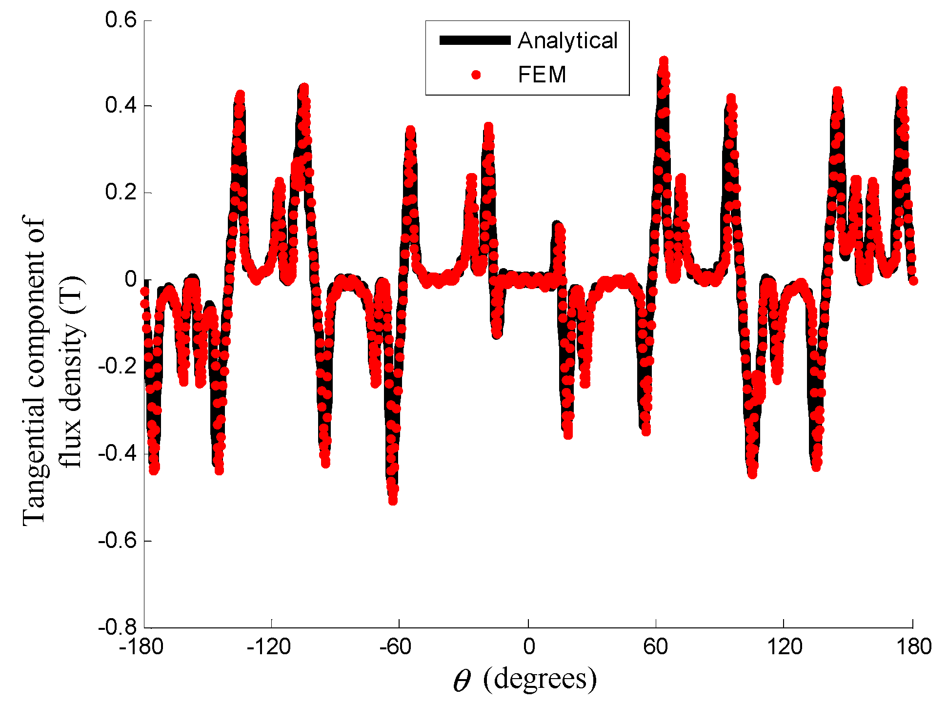
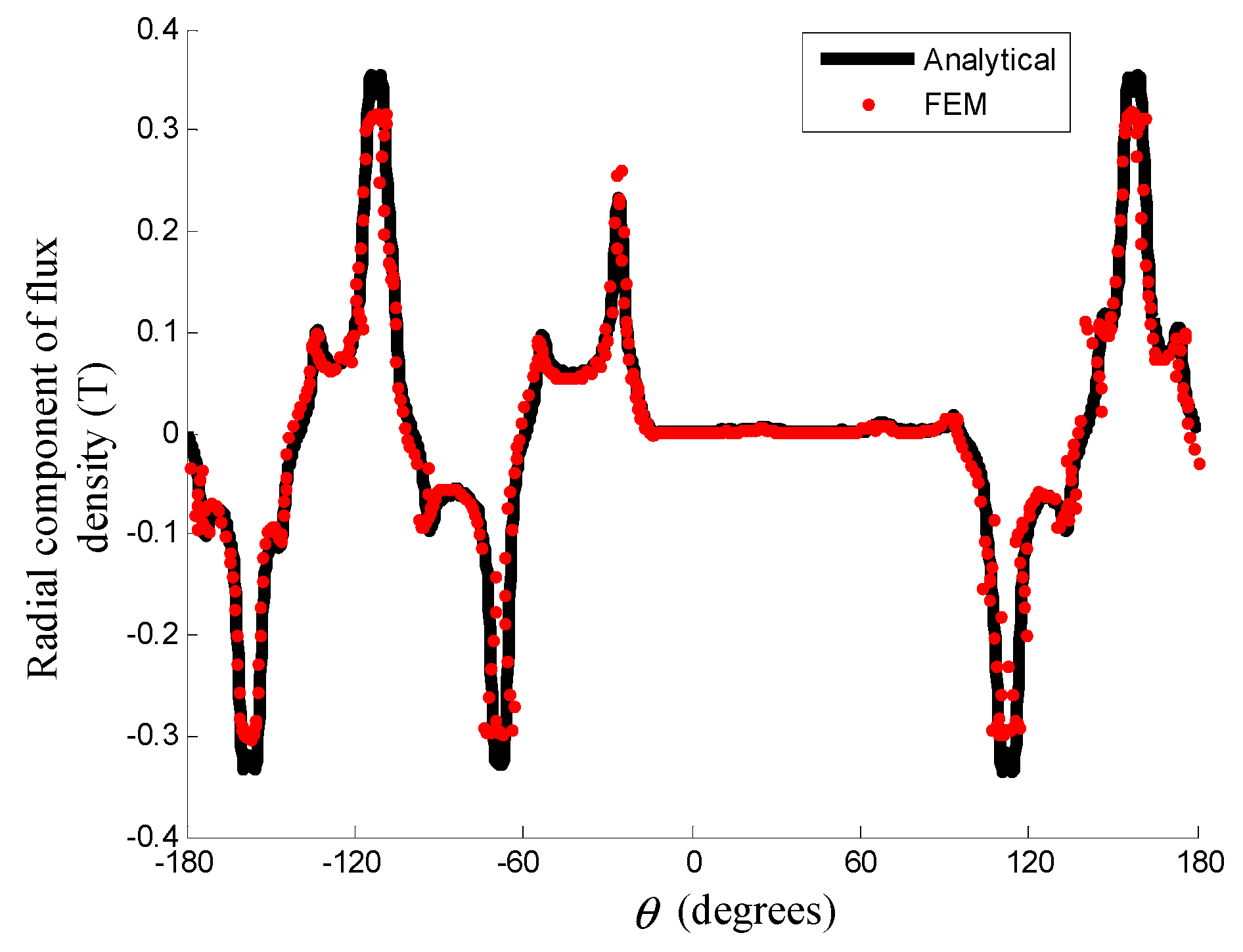
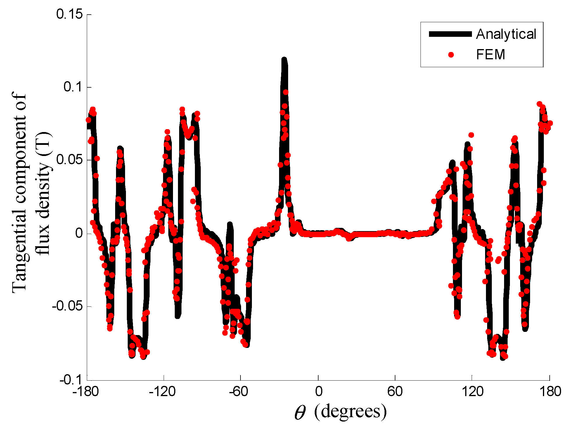
4.1. Flux Density
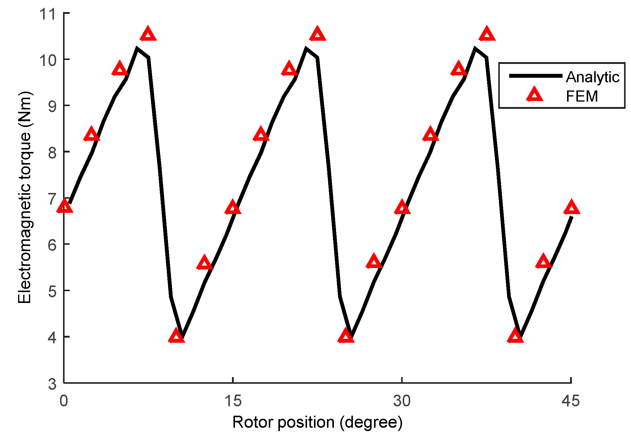
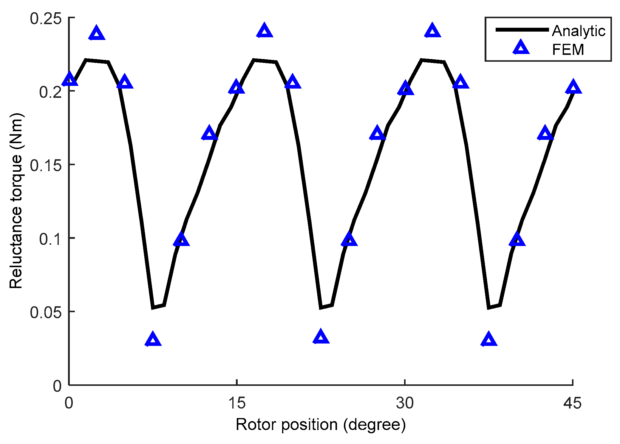
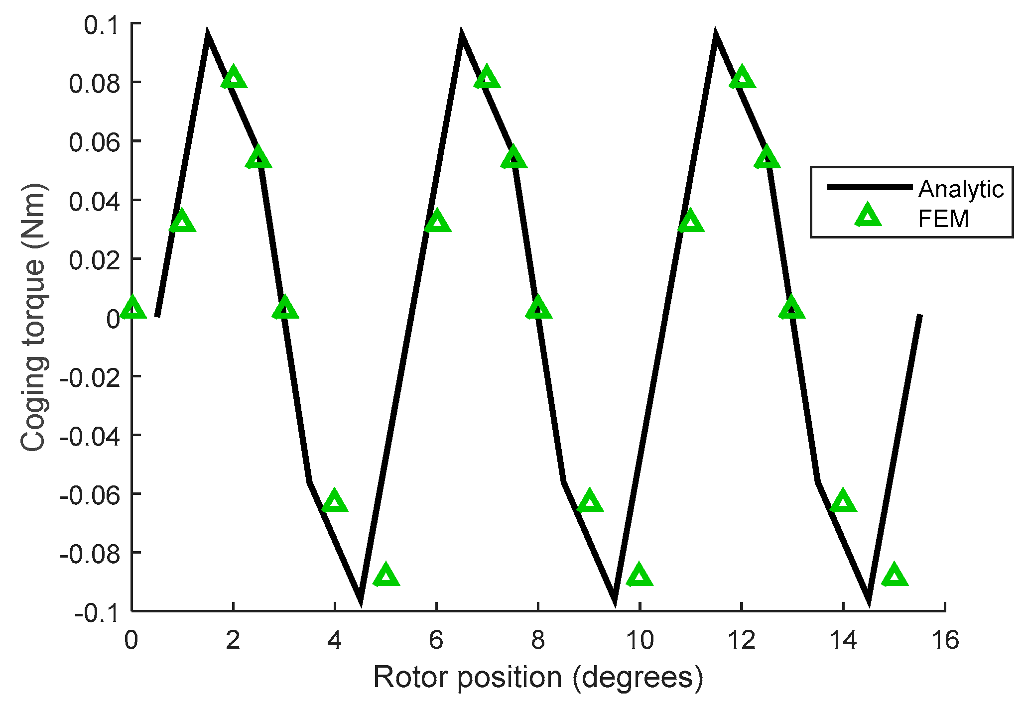
4.2. Torque
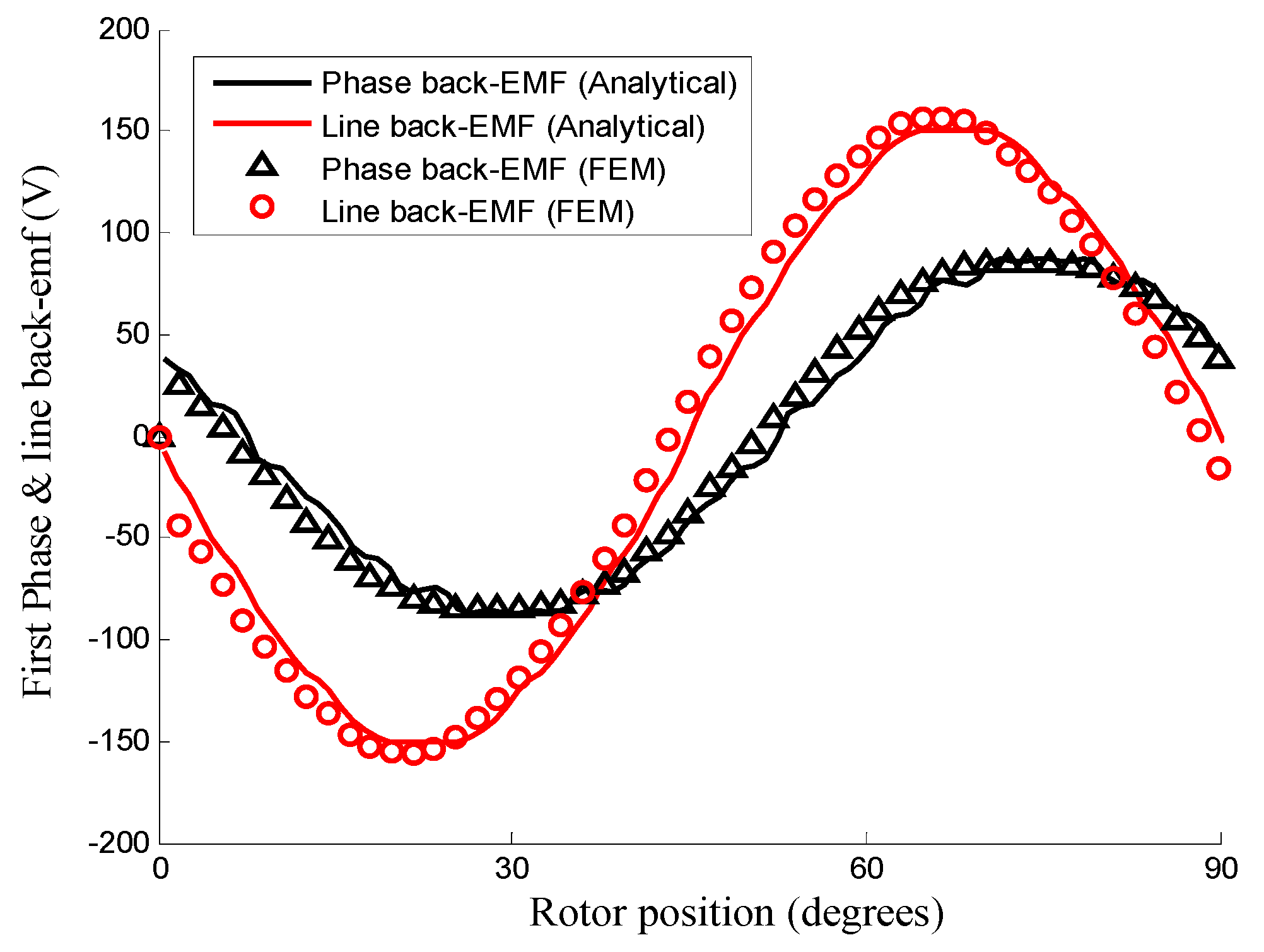
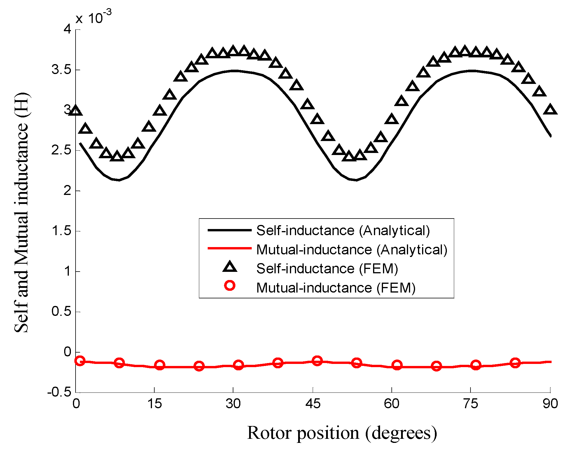
4.3. Back-EMF and Inductance
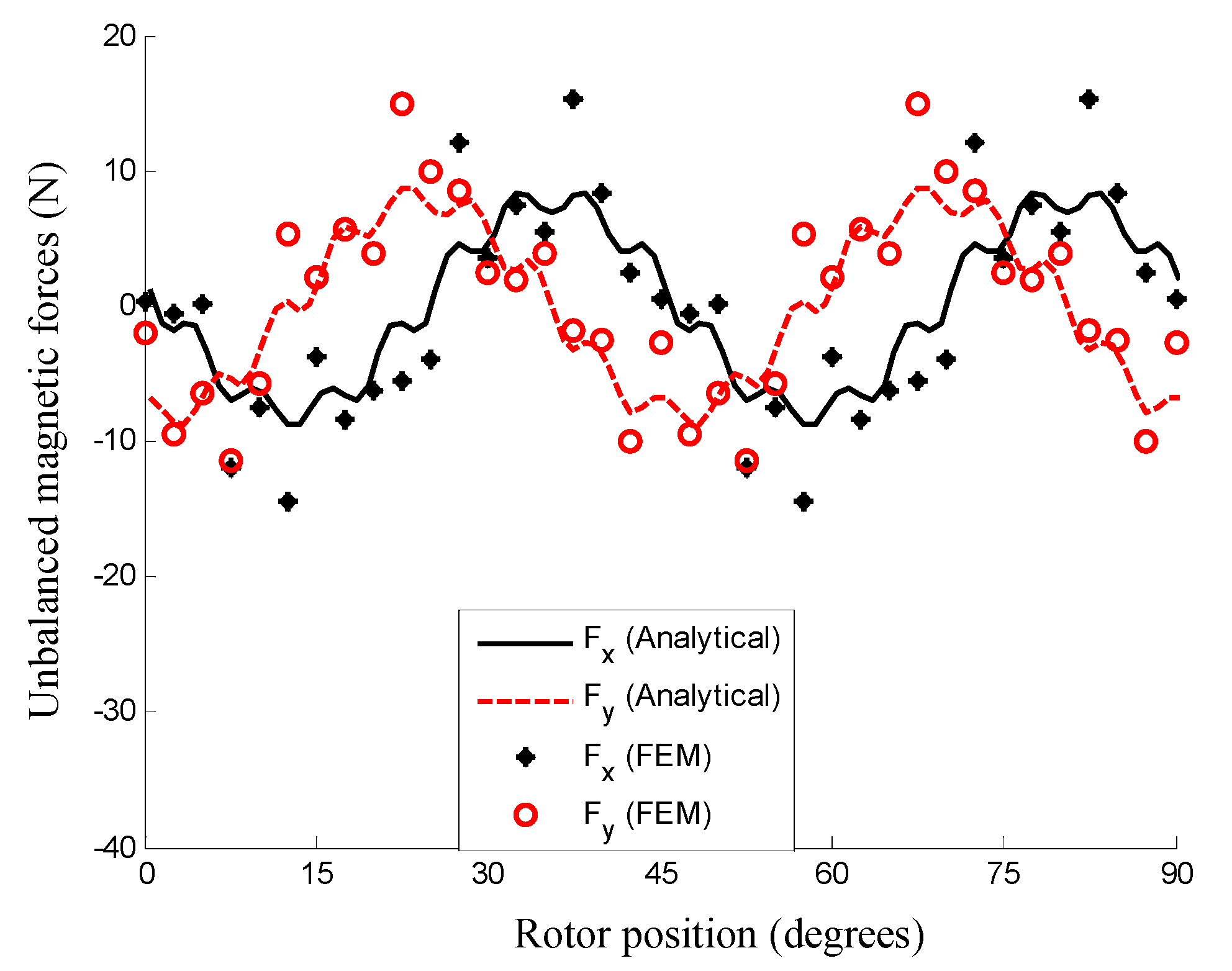
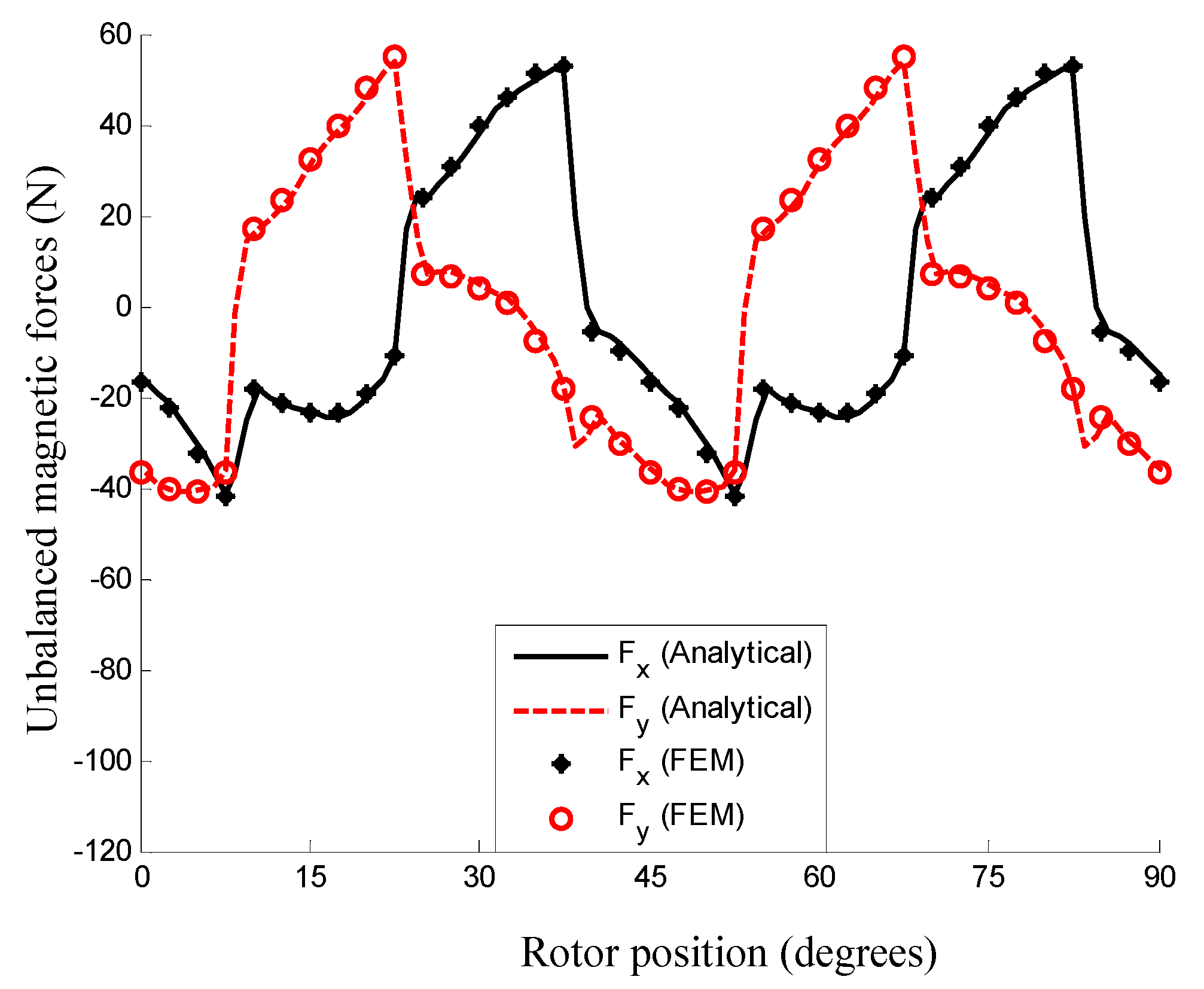
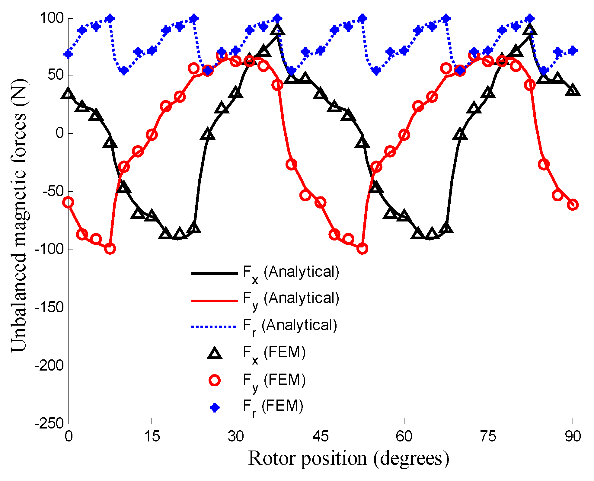
4.4. Unbalanced Magnetic Force (UMF)
5. Conclusions
Author Contributions
Conflicts of Interest
Appendix A
References
- Zarko, D.; Ban, D.; Lipo, T.A. Analytical calculation of magnetic field distribution in the slotted air gap of a surface permanent-magnet motor using complex relative air-gap permeance. IEEE Trans. Magn. 2006, 42, 1828–1837. [Google Scholar] [CrossRef]
- Hur, J.; Yoon, S.; Hwang, D.; Hyun, D. Analysis of PMLSM using three dimensional equivalent magnetic circuit network method. IEEE Trans. Magn. 1997, 33, 4143–4145. [Google Scholar]
- Rahideh, A.; Vahaj, A.A.; Mardaneh, M.; Lubin, T. Two-Dimensional Analytical Investigation of the Parameters and the Effects of Magnetisation Patterns on the Performance of Coaxial Magnetic Gears. IET Electr. Syst. Transp. 2017, 7, 230–245. [Google Scholar] [CrossRef]
- Moayed-Jahromi, H.; Rahideh, A.; Mardaneh, M. 2-D Analytical Model for External Rotor Brushless PM Machines. IEEE Trans. Energy Convers. 2016, 31, 1100–1109. [Google Scholar] [CrossRef]
- Wu, L.J.; Zhu, Z.Q.; Staton, D.; Popescu, M.; Hawkins, D. An improved subdomain model for predicting magnetic field of surface-mounted permanent-magnet machines accounting for toothtips. IEEE Trans. Magn. 2011, 47, 1693–1704. [Google Scholar] [CrossRef]
- Rahideh, A.; Korakianitis, T. Subdomain analytical magnetic field prediction of slotted brushless machines with surface mounted magnets. Int. Rev. Electr. Eng. 2012, 7, 3891–3909. [Google Scholar]
- Pourahmadi-Nakhli, M.; Rahideh, A.; Mardaneh, M. Analytical 2-D model of slotted brushless machines with cubic spoke-type permanent magnets. IEEE Trans. Energy Convers. 2018, 33, 373–382. [Google Scholar] [CrossRef]
- Boughrara, K.; Ibtiouen, R.; Lubin, T. Analytical Prediction of Magnetic Field in Parallel Double Excitation and Spoke-Type Permanent-Magnet Machines Accounting for Tooth-Tips and Shape of Polar Pieces. IEEE Trans. Magn. 2012, 48, 2121–2137. [Google Scholar] [CrossRef]
- Rahideh, A.; Korakianitis, T. Analytical magnetic field calculation of slotted brushless PM machines with surface inset magnets. IEEE Trans. Magn. 2012, 48, 2633–2649. [Google Scholar] [CrossRef]
- Dubas, F.; Sari, A.; Kauffmann, J.M.; Espanet, C. Cogging torque evaluation through a magnetic field analytical computation in permanent magnet motors. In Proceedings of the 2009 International Conference on Electrical Machines and Systems, Tokyo, Japan, 15–18 November 2009; pp. 1–5. [Google Scholar]
- Dubas, F.; Espanet, C. Semi-analytical Solution of 2-D rotor eddy-current losses due to the slotting effect in SMPMM. In Proceedings of the 17th Conference on the Computation of Electromagnetic Fields COMPUMAG 2009, Florianopolis, Brasil, 22–26 November 2009; pp. 20–25. [Google Scholar]
- Lubin, T.; Mezani, S.; Rezzoug, A. 2-D exact analytical model for surface-mounted permanent magnet motors with semi-closed slots. IEEE Trans. Magn. 2011, 47, 479–492. [Google Scholar] [CrossRef]
- Lubin, T.; Mezani, S.; Rezzoug, A. Two-dimensional analytical calculation of magnetic field and electromagnetic torque for surface-inset permanent magnet motors. IEEE Trans. Magn. 2012, 48, 2080–2091. [Google Scholar] [CrossRef]
- Dubas, F.; Espanet, C. Analytical solution of the magnetic field in permanent-magnet motors taking into account slotting effect: No-load vector potential and flux density calculation. IEEE Trans. Magn. 2009, 45, 2097–2109. [Google Scholar] [CrossRef]
- Zhu, Z.Q.; Wu, L.J.; Xia, Z.P. An accurate subdomain model for magnetic field computation in slotted surface mounted permanent-magnet machines. IEEE Trans. Magn. 2010, 46, 1100–1115. [Google Scholar] [CrossRef]
- Boughrara, K.; Chikouche, B.L.; Ibtiouen, R.; Zarko, D.; Touhami, O. Analytical model of slotted air-gap surface mounted permanent-magnet synchronous motor with magnet bars magnetized in the shifting direction. IEEE Trans. Magn. 2009, 45, 747–758. [Google Scholar] [CrossRef]
- Bellara, A.; Amara, Y.; Barakat, G.; Dakyo, B. Two-dimensional exact analytical solution of armature reaction field in slotted surface mounted PM radial flux synchronous machines. IEEE Trans. Magn. 2009, 45, 4534–4538. [Google Scholar] [CrossRef]
- Dubas, F.; Espanet, C.; Miraoui, A. Field diffusion equation in high-speed surface mounted permanent magnet motors, parasitic eddy-current losses. In Proceedings of the 6th International Symposium on Advanced Electromechanical Motion Systems, Lausanne, Switzerland, 27–29 September 2005; pp. 1–6. [Google Scholar]
- Liu, Z.J.; Li, J.T. Analytical solution of air-gap field in permanent-magnet motors taking into account the effect of pole transition over slots. IEEE Trans. Magn. 2007, 43, 3872–3883. [Google Scholar] [CrossRef]
- Zhu, Z.Q.; Howe, D.; Chan, C.C. Improved analytical model for predicting the magnetic field distribution in brushless permanent-magnet machines. IEEE Trans. Magn. 2002, 38, 229–238. [Google Scholar] [CrossRef]
- Rahideh, A.; Korakianitis, T. Analytical magnetic field distribution of slotless brushless machines with inset permanent magnets. IEEE Trans. Magn. 2011, 47, 1763–1774. [Google Scholar] [CrossRef]
- Dubas, F.; Rahideh, A. 2-D analytical PM eddy-current loss calculations in slotless PMSM equipped with surface-inset magnets. IEEE Trans. Magn. 2014, 50, 6300320. [Google Scholar] [CrossRef]
- Rahideh, A.; Korakianitis, T. Analytical open-circuit magnetic field distribution of slotless brushless permanent magnet machines with rotor eccentricity. IEEE Trans. Magn. 2011, 47, 4791–4808. [Google Scholar] [CrossRef]
- Rahideh, A.; Mardaneh, M.; Korakianitis, T. Analytical 2-D calculations of torque, inductance, and back-EMF for brushless slotless machines with surface inset magnets. IEEE Trans. Magn. 2013, 49, 4873–4884. [Google Scholar] [CrossRef]
- Rahideh, A.; Korakianitis, T. Analytical, armature reaction field distribution of slotless brushless machines with inset permanent magnets. IEEE Trans. Magn. 2012, 48, 2178–2191. [Google Scholar] [CrossRef]
- Atallah, K.; Zhu, Z.Q.; Howe, D.; Birch, T.S. Armature reaction field and winding inductances of slotless permanent-magnet brushless machines. IEEE Trans. Magn. 1998, 34, 3737–3744. [Google Scholar] [CrossRef]
- Pfister, P.D.; Perriard, Y. Slotless permanent-magnet machines: General analytical magnetic field calculation. IEEE Trans. Magn. 2011, 47, 1739–1752. [Google Scholar] [CrossRef]
- Holm, S.R.; Polinder, H.; Ferreira, J.A. Analytical modeling of a permanent-magnet synchronous machine in a flywheel. IEEE Trans. Magn. 2007, 43, 1955–1967. [Google Scholar] [CrossRef]
- Liu, Z.J.; Li, J.T. Accurate prediction of magnetic field and magnetic forces in permanent magnet motors using an analytical solution. IEEE Trans. Energy Convers. 2008, 23, 717–726. [Google Scholar] [CrossRef]
- Liu, Z.J.; Li, J.T.; Jiang, Q. An improved analytical solution for predicting magnetic forces in permanent magnet motors. J. Appl. Phys. 2008, 103, 07F135. [Google Scholar] [CrossRef]
- Amara, Y.; Reghem, P.; Barakat, G. Analytical prediction of eddy-current loss in armature windings of permanent magnet brushless AC machines. IEEE Trans. Magn. 2010, 46, 3481–3484. [Google Scholar] [CrossRef]
- Pfister, P.; Yin, X.; Fang, Y. Slotted Permanent-Magnet Machines: General Analytical Model of Magnetic Fields, Torque, Eddy Currents, and Permanent-Magnet Power Losses Including the Diffusion Effect. IEEE Trans. Magn. 2016, 52, 1–13. [Google Scholar] [CrossRef]
- Wu, L.J.; Zhu, Z.Q.; Staton, D.; Popescu, M.; Hawkins, D. Subdomain model for predicting armature reaction field of surface-mounted permanent-magnet machines accounting for tooth-tips. IEEE Trans. Magn. 2011, 47, 812–822. [Google Scholar] [CrossRef]
- Gysen, B.L.J.; Meessen, K.J.; Paulides, J.J.H.; Lomonova, E.A. General formulation of the electromagnetic field distribution in machines and devices using fourier analysis. IEEE Trans. Magn. 2010, 46, 39–52. [Google Scholar] [CrossRef]
- Zhu, Z.Q.; Howe, D.; Xia, Z.P. Prediction of open-circuit airgap field distribution in brushless machines having an inset permanent magnet rotor topology. IEEE Trans. Magn. 1994, 30, 98–107. [Google Scholar] [CrossRef]
- Jian, L.; Chau, K.T.; Gong, Y.; Yu, C.; Li, W. Analytical calculation of magnetic field in surface-inset permanent-magnet motors. IEEE Trans. Magn. 2009, 45, 4688–4691. [Google Scholar] [CrossRef]
- Zhu, Z.Q.; Ishak, D.; Howe, D.; Chen, J. Unbalanced magnetic forces in permanent-magnet brushless machines with diametrically asymmetric phase windings. IEEE Trans. Ind. Appl. 2007, 43, 1544–1553. [Google Scholar] [CrossRef]
- Sprangers, R.L.J.; Paulides, J.J.H.; Gysen, B.L.J.; Lomonova, E.A. Magnetic Saturation in Semi-Analytical Harmonic Modeling for Electric Machine Analysis. IEEE Trans. Magn. 2016, 52, 1–10. [Google Scholar] [CrossRef]
- Dubas, F.; Boughrara, K. New scientific contribution on the 2-D subdomain technique in polar coordinates: Taking into account of iron parts. Math. Comput. Appl. 2017, 22, 42. [Google Scholar] [CrossRef]
- Dubas, F.; Boughrara, K. New scientific contribution on the 2-D subdomain technique in Cartesian coordinates: Taking into account of iron parts. Math. Comput. Appl. 2017, 22, 17. [Google Scholar] [CrossRef]
- Djelloul-Khedda, Z.; Boughrara, K.; Dubas, F.; Kechroud, A.; Tikellaline, A. Analytical Prediction of Iron-Core Losses in Flux-Modulated Permanent-Magnet Synchronous Machines. IEEE Trans. Magn. 2019, 55, 1–12. [Google Scholar] [CrossRef]
- Djelloul-Khedda, Z.; Boughrara, K.; Dubas, F.; Ibtiouen, R. Nonlinear Analytical Prediction of Magnetic Field and Electromagnetic Performances in Switched Reluctance Machines. IEEE Trans. Magn. 2017, 53, 1–11. [Google Scholar] [CrossRef]
- Djelloul-Khedda, Z.; Boughrara, K.; Dubas, F.; Kechroud, A.; Souleyman, B. Semi-Analytical Magnetic Field Predicting in Many Structures of Permanent-Magnet Synchronous Machines Considering the Iron Permeability. IEEE Trans. Magn. 2018, 54, 1–21. [Google Scholar] [CrossRef]
- Roubache, L.; Boughrara, K.; Dubas, F.; Ibtiouen, R. New Subdomain Technique for Electromagnetic Performances Calculation in Radial-Flux Electrical Machines Considering Finite Soft-Magnetic Material Permeability. IEEE Trans. Magn. 2018, 54, 1–15. [Google Scholar] [CrossRef]
- Ben Yahia, M.; Boughrara, K.; Dubas, F.; Roubache, L.; Ibtiouen, R. Two-Dimensional Exact Subdomain Technique of Switched Reluctance Machines with Sinusoidal Current Excitation. Math. Comput. Appl. 2018, 23, 59. [Google Scholar]
- Roubache, L.; Boughrara, K.; Dubas, F.; Ibtiouen, R. Elementary subdomain technique for magnetic field calculation in rotating electrical machines with local saturation effect. Int. J. Comput. Math. Electr. Electron. Eng. 2018. [Google Scholar] [CrossRef]
- Boughrara, K.; Dubas, F.; Ibtiouen, R. 2-D Exact Analytical Method for Steady-State Heat Transfer Prediction in Rotating Electrical Machines. IEEE Trans. Magn. 2018, 54, 1–19. [Google Scholar] [CrossRef]
- Hannon, B.; Sergeant, P.; Dupré, L. Two-dimensional Fourier-based modeling of electric machines. In Proceedings of the 2017 IEEE International Electric Machines and Drives Conference, Miami, FL, USA, 21–24 May 2017; pp. 1–8. [Google Scholar]
- Lubin, T.; Rezzoug, A. 3-D Analytical Model for Axial-Flux Eddy-Current Couplings and Brakes Under Steady-State Conditions. IEEE Trans. Magn. 2015, 51, 1–12. [Google Scholar] [CrossRef]
- Lubin, T.; Rezzoug, A. Improved 3-D Analytical Model for Axial-Flux Eddy-Current Couplings with Curvature Effects. IEEE Trans. Magn. 2017, 53, 1–9. [Google Scholar] [CrossRef]
- Zarko, D.; Ban, D.; Lipo, T.A. Analytical solution for cogging torque in surface permanent magnet motors using conformal mapping. IEEE Trans. Magn. 2008, 44, 52–65. [Google Scholar] [CrossRef]
- Boughrara, K.; Zarko, D.; Ibtiouen, R.; Touhami, O.; Rezzoug, A. Magnetic field analysis of inset and surface-mounted permanent-magnet synchronous motors using Schwarz–Christoffel transformation. IEEE Trans. Magn. 2009, 45, 3166–3178. [Google Scholar] [CrossRef]
- Clemens, M.; Lang, J.; Teleaga, D.; Wimmer, G. Transient 3D magnetic field simulations with combined space and time mesh adaptivity for lowest order Whitney finite element formulations. IET Sci. Meas. Technol. 2009, 3, 377–383. [Google Scholar] [CrossRef]
- Liang, Y.; Bian, X.; Yang, L.; Wu, L. Numerical calculation of circulating current losses in stator transposition bar of large hydro-generator. IET Sci. Meas. Technol. 2015, 9, 485–491. [Google Scholar] [CrossRef]
- Mohammed, O.A.; Liu, S.; Liu, Z. FE-based physical phase variable model of PM synchronous machines under stator winding short circuit faults. IET Sci. Meas. Technol. 2007, 1, 12–16. [Google Scholar] [CrossRef]


| Sub-Domain | Symbol | Number of Sub-Regions |
|---|---|---|
| Magnet | ||
| Air-gap | 1 | |
| Slot-opening | so | |
| Slot |
| Magnetization Pattern | Illustration | Radial Waveform Component | Tangential Waveform Component | Coefficient of the Radial Component | Coefficient of the Tangential Component |
| Radial Magnetization |  | 0 | |||
| Parameters | Unit | Symbol | Value |
|---|---|---|---|
| Number of phases | 3 | ||
| Number of the pole-pair | 4 | ||
| Number of slots | 9 | ||
| Outer radius of the slots | (mm) | 18 | |
| Outer radius of the slot-opening | (mm) | 29 | |
| Stator radius | (mm) | 31 | |
| Magnet radius | (mm) | 32 | |
| Radius of the rotor back iron | (mm) | 38 | |
| Axial length | (m) | Ls | 0.1 |
| Span of the slot | (rad) | 0.6 | |
| Span of the slot-opening | (rad) | 0.3 | |
| Pole arc to pole pith of the magnet | 0.85 | ||
| Ratio of the rotor back iron to the pole pitch | 0.85 | ||
| Remanence of magnet | (T) | 1 | |
| Relative permeability of the magnet | 1.05 | ||
| Number of harmonics in each sub-domain | N, U, V, W | 100 |
© 2019 by the authors. Licensee MDPI, Basel, Switzerland. This article is an open access article distributed under the terms and conditions of the Creative Commons Attribution (CC BY) license (http://creativecommons.org/licenses/by/4.0/).
Share and Cite
Vahaj, A.; Rahideh, A.; Moayed-Jahromi, H.; Ghaffari, A. Exact Two-Dimensional Analytical Calculations for Magnetic Field, Electromagnetic Torque, UMF, Back-EMF, and Inductance of Outer Rotor Surface Inset Permanent Magnet Machines. Math. Comput. Appl. 2019, 24, 24. https://0-doi-org.brum.beds.ac.uk/10.3390/mca24010024
Vahaj A, Rahideh A, Moayed-Jahromi H, Ghaffari A. Exact Two-Dimensional Analytical Calculations for Magnetic Field, Electromagnetic Torque, UMF, Back-EMF, and Inductance of Outer Rotor Surface Inset Permanent Magnet Machines. Mathematical and Computational Applications. 2019; 24(1):24. https://0-doi-org.brum.beds.ac.uk/10.3390/mca24010024
Chicago/Turabian StyleVahaj, AmirAbbas, Akbar Rahideh, Hossein Moayed-Jahromi, and AliReza Ghaffari. 2019. "Exact Two-Dimensional Analytical Calculations for Magnetic Field, Electromagnetic Torque, UMF, Back-EMF, and Inductance of Outer Rotor Surface Inset Permanent Magnet Machines" Mathematical and Computational Applications 24, no. 1: 24. https://0-doi-org.brum.beds.ac.uk/10.3390/mca24010024