Natural Frequency Analysis of Functionally Graded Orthotropic Cross-Ply Plates Based on the Finite Element Method

Abstract

This paper aims to present a finite element (FE) formulation for the study of the natural frequencies of functionally graded orthotropic laminated plates characterized by cross-ply layups. A nine-node Lagrange element is considered for this purpose. The main novelty of the research is the modelling of the reinforcing fibers of the orthotropic layers assuming a non-uniform distribution in the thickness direction. The Halpin–Tsai approach is employed to define the overall mechanical properties of the composite layers starting from the features of the two constituents (fiber and epoxy resin). Several functions are introduced to describe the dependency on the thickness coordinate of their volume fraction. The analyses are carried out in the theoretical framework provided by the first-order shear deformation theory (FSDT) for laminated thick plates. Nevertheless, the same approach is used to deal with the vibration analysis of thin plates, neglecting the shear stiffness of the structure. This objective is achieved by properly choosing the value of the shear correction factor, without any modification in the formulation. The results prove that the dynamic response of thin and thick plates, in terms of natural frequencies and mode shapes, is affected by the non-uniform placement of the fibers along the thickness direction.

1. Introduction

The finite element (FE) method currently represents the most-utilized computational approach to solve several engineering problems and in applications whose solutions cannot be obtained analytically [1]. The technological advancements in computer sciences have allowed a fast and easy diffusion of this technique, especially in terms of structural mechanics problems. The key to the success of the FE method lies in the reduction of complex problems into simpler ones in which the reference domain is made of several discrete elements, and in its easy computational implementation. This idea was first highlighted by Duncan and Collar [2,3], and successively emphasized by Hrennikoff [4], Courant [5], Clough [6], and Melosh [7].

The approximate solutions that can be obtained by means of the FE approach are accurate and representative of the physical problem under consideration [8,9]. To the best of the authors’ knowledge, the progression and development of this technique are well-described in many pertinent books, such as the ones by Oden [10], Oden and Reddy [11], Hinton [12], Zienkiewicz [13], Reddy [14], Onate [15], Hughes [16], and Ferreira [17]. These books should be used as references for the theoretical background of the numerical approach at issue. For completeness purposes, it should be recalled that various and alternative approaches have been developed in past decades to obtain approximated but accurate solutions to several complex structural problems, not only based on the FE method [18,19,20,21].

An intriguing application that is efficiently solved by means of the FE methodology is about the structural response of plates and panels made of composite materials [22,23,24]. With respect to an isotropic and conventional medium, a composite material can reach superior performance by combining two (or more) constituents. A typical example of this category are fiber-reinforced composites, in which the high-strength fibers are the main load-carrying elements, whereas the matrix has the task of keeping them together and protecting the reinforcing phase from the environment [25,26,27,28]. In general, a micromechanical approach should be employed to evaluate the overall mechanical properties of these materials, starting from the features of the single constituents. The review paper by Chamis and Sendeckyj represents a fundamental contribution is this direction [29]. One of the most effective approaches that can be used toward this aim is the one proposed by Halpin [30] and Tsai [31,32], who developed a semi-empirical method and expressed the mechanical properties of the constituents in terms of Hill’s elastic moduli [33,34]. Further details concerning the micromechanics of fiber-reinforced composite materials can be found in [35].

The use of a versatile numerical method also allows us to investigate the structural response of composite structures with non-uniform mechanical properties. In particular, in the present paper the reinforcing fibers are characterized by a gradual variation of their volume fraction along the plate thickness, following the same idea of functionally graded materials [36,37,38,39,40,41,42,43,44,45,46,47,48,49,50,51,52]. With respect to this class of materials, in which the composites turn out to be isotropic, the layers of the plate assume orthotropic features and can also be oriented. This topic clearly falls within the aim of the optimal design of composite structures [53,54,55,56,57,58]. It should be mentioned that a similar approach is followed in the design of functionally graded carbon-nanotube-reinforced composites, due to the advancements in nanostructures and nanotechnologies [59,60,61,62,63,64,65,66,67,68].

In this paper, the research is organized in two main sections. After this brief introduction, the FE formulation for laminated thick and thin plates is presented in Section 2. Here, the theoretical framework is based on the well-known first-order shear deformation theory (FSDT) for laminated composite structures [69,70]. The effect of the shear correction factor is also discussed in order to deal with thin plates [71]. In addition, the micromechanics approach based on the Halpin–Tsai model is described in detail, by also introducing the topic of variable mechanical properties. 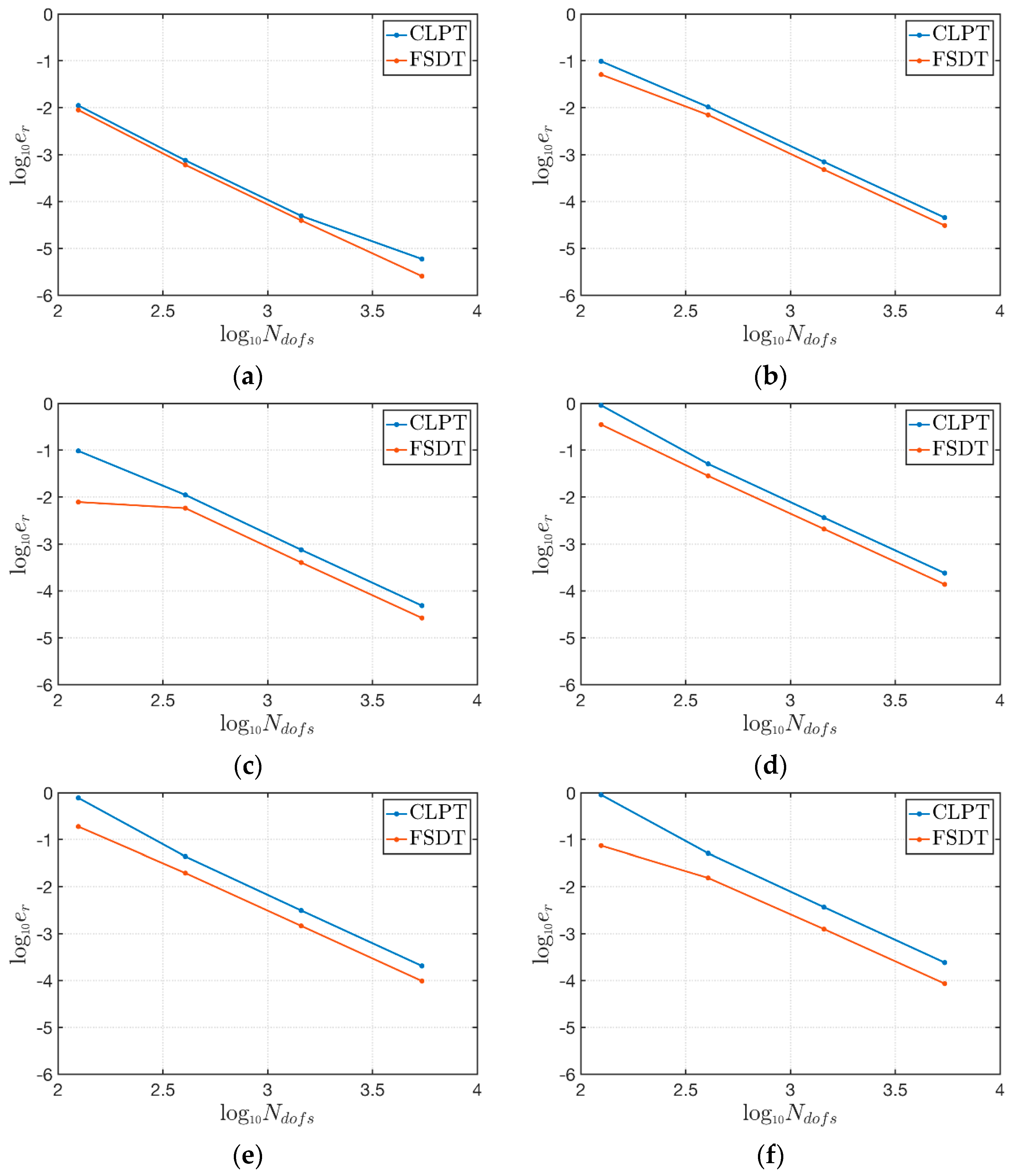Section 3 presents the results of the numerical applications. As a preliminary test, the accuracy and convergence features of the numerical approach are discussed by means of the comparison with the semi-analytical solutions available in the literature for thin and thick laminated composite plates. Then, the natural frequencies of functionally graded orthotropic cross-ply plates are presented for several mechanical configurations. Finally, Appendix A is added to define the terms of the fundamental operators of the proposed FE formulation.

2. Finite Element (FE) Formulation for Laminated Thick and Thin Plates

The theoretical framework of the current research is based on the first-order shear deformation theory (FSDT). The governing equations are presented in this section by developing the corresponding FE formulation. The following kinematic model is assumed within each discrete element of the plate [69]:

$$\begin{array}{l}{U}_x^{\left(e\right)}\left(x,y,z,t\right)=u_x^{\left(e\right)}\left(x,y,t\right)+z{\varphi }_x^{\left(e\right)}\left(x,y,t\right)\\ U_y^{\left(e\right)}\left(x,y,z,t\right)=u_y^{\left(e\right)}\left(x,y,t\right)+z{\varphi }_y^{\left(e\right)}\left(x,y,t\right)\\ U_z^{\left(e\right)}\left(x,y,z,t\right)=u_z^{\left(e\right)}\left(x,y,t\right)\end{array},$$

(1)

where $U_x^{\left(e\right)},U_y^{\left(e\right)},U_z^{\left(e\right)}$ are the three-dimensional displacements of the structure, whereas the degrees of freedom of the problem are given by three translations $u_x^{\left(e\right)},u_y^{\left(e\right)},u_z^{\left(e\right)}$ and two rotations ${\varphi }_x^{\left(e\right)},{\varphi }_y^{\left(e\right)}$ defined on the plate middle surface. These quantities can be conveniently collected in the corresponding vector $u^{\left(e\right)}$, defined below

$$u^{\left(e\right)}={\left[\begin{array}{ccccc}{u}_x^{\left(e\right)}& u_y^{\left(e\right)}& u_z^{\left(e\right)}& {\varphi }_x^{\left(e\right)}& {\varphi }_y^{\left(e\right)}\end{array}\right]}^T.$$

(2)

The coordinates $x,y,z$ specify the local reference system of the plate and $t$ is the time variable. The superscript $\left(e\right)$ clearly specifies that this model is valid for each element. The geometry of the plate is fully described once the lengths $L_x,L_y$ of its sides and its overall thickness $h$ are defined. It should be recalled that for a laminate structure one gets

$$h={\displaystyle \sum _{k=1}^{N_L}\left(z_{k+1}-z_k\right)},$$

(3)

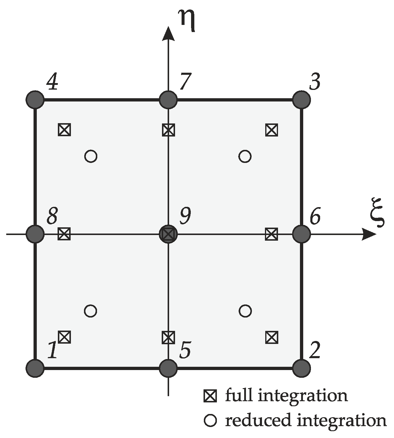
in which $z_{k+1},z_k$ stand for the upper and lower coordinates of the $k$-th layer, respectively. The degrees of the freedom (2) are approximated in each element by means of quadratic Lagrange interpolation functions. As can be noted from Figure 1, nine nodes are introduced in each subdomain. As a consequence, the degrees of freedom assume the following aspect:

$$\begin{array}{l}{u}_x^{\left(e\right)}\left(x,y,t\right)={\displaystyle \sum _{i=1}^9{N}_i\left(x,y\right)u_{x,i}^{\left(e\right)}\left(t\right)}=\overline{N}{u}_x^{\left(e\right)}\\ u_y^{\left(e\right)}\left(x,y,t\right)={\displaystyle \sum _{i=1}^9{N}_i\left(x,y\right)u_{y,i}^{\left(e\right)}\left(t\right)}=\overline{N}{u}_y^{\left(e\right)}\\ u_z^{\left(e\right)}\left(x,y,t\right)={\displaystyle \sum _{i=1}^9{N}_i\left(x,y\right)u_{z,i}^{\left(e\right)}\left(t\right)}=\overline{N}{u}_z^{\left(e\right)}\\ {\varphi }_x^{\left(e\right)}\left(x,y,t\right)={\displaystyle \sum _{i=1}^9{N}_i\left(x,y\right){\varphi }_{x,i}^{\left(e\right)}\left(t\right)}=\overline{N}{\mathsf{\varphi }}_x^{\left(e\right)}\\ {\varphi }_y^{\left(e\right)}\left(x,y,t\right)={\displaystyle \sum _{i=1}^9{N}_i\left(x,y\right){\varphi }_{y,i}^{\left(e\right)}\left(t\right)}=\overline{N}{\mathsf{\varphi }}_y^{\left(e\right)}\end{array},$$

(4)

where $N_i$ represents the $i$-th shape function, whereas $u_{x,i}^{\left(e\right)},u_{y,i}^{\left(e\right)},u_{z,i}^{\left(e\right)},{\varphi }_{x,i}^{\left(e\right)},{\varphi }_{y,i}^{\left(e\right)}$ denote the nodal displacements, which can be included in the corresponding vectors

$$\begin{array}{c}{u}_x^{\left(e\right)}={\left[\begin{array}{ccc}{u}_{x,1}^{\left(e\right)}& \cdots & u_{x,9}^{\left(e\right)}\end{array}\right]}^T,\hspace{1em}{u}_y^{\left(e\right)}={\left[\begin{array}{ccc}{u}_{y,1}^{\left(e\right)}& \cdots & u_{y,9}^{\left(e\right)}\end{array}\right]}^T,\hspace{1em}{u}_z^{\left(e\right)}={\left[\begin{array}{ccc}{u}_{z,1}^{\left(e\right)}& \cdots & u_{z,9}^{\left(e\right)}\end{array}\right]}^T\\ {\mathsf{\varphi }}_x^{\left(e\right)}={\left[\begin{array}{ccc}{\varphi }_{x,1}^{\left(e\right)}& \cdots & {\varphi }_{x,9}^{\left(e\right)}\end{array}\right]}^T,\hspace{1em}{\mathsf{\varphi }}_y^{\left(e\right)}={\left[\begin{array}{ccc}{\varphi }_{y,1}^{\left(e\right)}& \cdots & {\varphi }_{y,9}^{\left(e\right)}\end{array}\right]}^T\end{array}.$$

(5)

On the other hand, the shape functions linked to the nine nodes of the finite element are included in the vector $\overline{N}$, defined below:

$$\overline{N}=\left[\begin{array}{ccc}{N}_1& \cdots & N_9\end{array}\right].$$

(6)

For the sake of clarity, it should be recalled that the nodes are identified in each element by following the numbering specified in Figure 1.

At this point, the nodal degrees of freedom can be collected in a sole vector ${\overline{u}}^{\left(e\right)}$ to simplify the nomenclature:

$$\begin{array}{ll}{\overline{u}}^{\left(e\right)}& ={\left[\begin{array}{ccccc}{u}_x^{\left(e\right)}& u_y^{\left(e\right)}& u_z^{\left(e\right)}& {\mathsf{\varphi }}_x^{\left(e\right)}& {\mathsf{\varphi }}_y^{\left(e\right)}\end{array}\right]}^T\\ & ={\left[\begin{array}{ccccccccccccccc}{u}_{x,1}^{\left(e\right)}& \cdots & u_{x,9}^{\left(e\right)}& u_{y,1}^{\left(e\right)}& \cdots & u_{y,9}^{\left(e\right)}& u_{z,1}^{\left(e\right)}& \cdots & u_{z,9}^{\left(e\right)}& {\varphi }_{x,1}^{\left(e\right)}& \cdots & {\varphi }_{x,9}^{\left(e\right)}& {\varphi }_{y,1}^{\left(e\right)}& \cdots & {\varphi }_{y,9}^{\left(e\right)}\end{array}\right]}^T\end{array},$$

(7)

and to write the definitions (4) by using the following matrix notation:

$$\left[\begin{array}{c}{u}_x^{\left(e\right)}\\ u_y^{\left(e\right)}\\ u_z^{\left(e\right)}\\ {\varphi }_x^{\left(e\right)}\\ {\varphi }_y^{\left(e\right)}\end{array}\right]=\left[\begin{array}{ccccc}\overline{N}& 0& 0& 0& 0\\ 0& \overline{N}& 0& 0& 0\\ 0& 0& \overline{N}& 0& 0\\ 0& 0& 0& \overline{N}& 0\\ 0& 0& 0& 0& \overline{N}\end{array}\right]\left[\begin{array}{c}{u}_x^{\left(e\right)}\\ u_y^{\left(e\right)}\\ u_z^{\left(e\right)}\\ {\mathsf{\varphi }}_x^{\left(e\right)}\\ {\mathsf{\varphi }}_y^{\left(e\right)}\end{array}\right]\hspace{1em}\iff \hspace{1em}\underset{5\times 1}{u^{\left(e\right)}}=\underset{5\times \left(9\times 5\right)}{N}\underset{\left(9\times 5\right)\times 1}{{\overline{u}}^{\left(e\right)}}.$$

(8)

The size of each matrix is indicated under the corresponding symbol. It is important to specify that the same approximation is employed for all degrees of freedom (both translational and rotational displacements).

As mentioned in the books by Reddy [14] and Ferreira [17], it is convenient to introduce the natural coordinates $\xi ,\eta$ within the reference finite element, which is called the master element (or parent element). In this reference system, which is also depicted in Figure 1, the shape functions $N_i=N_i\left(\xi ,\eta \right)$ assume the following definitions:

$$\begin{array}{lll}{N}_1=\frac{1}{4}\left({\xi }^2-\xi \right)\left({\eta }^2-\eta \right)& N_2=\frac{1}{4}\left({\xi }^2+\xi \right)\left({\eta }^2-\eta \right)& N_3=\frac{1}{4}\left({\xi }^2+\xi \right)\left({\eta }^2+\eta \right)\\ N_4=\frac{1}{4}\left({\xi }^2-\xi \right)\left({\eta }^2+\eta \right)& N_5=\frac{1}{2}\left(1-{\xi }^2\right)\left({\eta }^2-\eta \right)& N_6=\frac{1}{2}\left({\xi }^2+\xi \right)\left(1-{\eta }^2\right)\\ N_7=\frac{1}{2}\left(1-{\xi }^2\right)\left({\eta }^2+\eta \right)& N_8=\frac{1}{2}\left({\xi }^2-\xi \right)\left(1-{\eta }^2\right)& N_9=\left(1-{\xi }^2\right)\left(1-{\eta }^2\right)\end{array},$$

(9)

for $\xi ,\eta \in \left[-1,1\right]$. The same functions are also used to describe the geometry of each discrete element according to the principles of the isoparametric FE formulation. The coordinate change between the physical domain and the parent element is accomplished through the relations shown below

$$x^{\left(e\right)}={\displaystyle \sum _{i=1}^9{N}_i\left(\xi ,\eta \right)x_i^{\left(e\right)}},\hspace{1em}{y}^{\left(e\right)}={\displaystyle \sum _{i=1}^9{N}_i\left(\xi ,\eta \right)y_i^{\left(e\right)}},$$

(10)

where the couple $x_i^{\left(e\right)},y_i^{\left(e\right)}$ defines the coordinates of the $i$-th node of the generic element. For the sake of conciseness, these quantities can be collected in the corresponding vectors $x^{\left(e\right)},y^{\left(e\right)}$:

$$x^e={\left[\begin{array}{ccc}{x}_1^{\left(e\right)}& \cdots & x_9^{\left(e\right)}\end{array}\right]}^T,\hspace{1em}{y}^e={\left[\begin{array}{ccc}{y}_1^{\left(e\right)}& \cdots & y_9^{\left(e\right)}\end{array}\right]}^T.$$

(11)

The Jacobian matrix $J$ related to the coordinate change (10) can be now introduced in order to evaluate the derivatives with respect to the natural coordinates of the parent element:

$$J=\left[\begin{array}{cc}\frac{\partial x^{\left(e\right)}}{\partial \xi }& \frac{\partial y^{\left(e\right)}}{\partial \xi }\\ \frac{\partial x^{\left(e\right)}}{\partial \eta }& \frac{\partial y^{\left(e\right)}}{\partial \eta }\end{array}\right]=\left[\begin{array}{cc}{\displaystyle \sum _{i=1}^9{x}_i^{\left(e\right)}}\frac{\partial N_i}{\partial \xi }& {\displaystyle \sum _{i=1}^9{y}_i^{\left(e\right)}}\frac{\partial N_i}{\partial \xi }\\ {\displaystyle \sum _{i=1}^9{x}_i^{\left(e\right)}}\frac{\partial N_i}{\partial \eta }& {\displaystyle \sum _{i=1}^9{y}_i^{\left(e\right)}}\frac{\partial N_i}{\partial \eta }\end{array}\right]=\left[\begin{array}{c}{B}_{\xi }\\ B_{\eta }\end{array}\right]\left[\begin{array}{cc}{x}^{\left(e\right)}& y^{\left(e\right)}\end{array}\right]=\left[\begin{array}{cc}{B}_{\xi }{x}^{\left(e\right)}& B_{\xi }{y}^{\left(e\right)}\\ B_{\eta }{x}^{\left(e\right)}& B_{\eta }{y}^{\left(e\right)}\end{array}\right],$$

(12)

where the vectors $B_{\xi },B_{\eta }$ collect the derivatives of the shape functions (9) with respect to $\xi ,\eta$

$$B_{\xi }=\left[\begin{array}{ccc}\frac{\partial N_1}{\partial \xi }& \cdots & \frac{N_9}{\partial \xi }\end{array}\right],\hspace{1em}{B}_{\eta }=\left[\begin{array}{ccc}\frac{\partial N_1}{\partial \eta }& \cdots & \frac{N_9}{\partial \eta }\end{array}\right].$$

(13)

At this point, the compatibility equations can be presented to define the strain components in each element. In particular, the membrane strains are given by

$${\epsilon }_x^{\left(e\right)}=\frac{\partial u_x^{\left(e\right)}}{\partial x}=B_x{u}_x^{\left(e\right)},\hspace{1em}{\epsilon }_y^{\left(e\right)}=\frac{\partial u_y^{\left(e\right)}}{\partial y}=B_y{u}_y^{\left(e\right)},\hspace{1em}{\gamma }_{xy}^{\left(e\right)}=\frac{\partial u_y^{\left(e\right)}}{\partial x}+\frac{\partial u_x^{\left(e\right)}}{\partial y}=B_x{u}_y^{\left(e\right)}+B_y{u}_x^{\left(e\right)}.$$

(14)

On the other hand, the bending and twisting curvatures can be defined as follows:

$$k_x^{\left(e\right)}=\frac{\partial {\varphi }_x^{\left(e\right)}}{\partial x}=B_x{\mathsf{\varphi }}_x^{\left(e\right)},\hspace{1em}{k}_y^{\left(e\right)}=\frac{\partial {\varphi }_y^{\left(e\right)}}{\partial y}=B_y{\mathsf{\varphi }}_y^{\left(e\right)},\hspace{1em}{k}_{xy}^{\left(e\right)}=\frac{\partial {\varphi }_y^{\left(e\right)}}{\partial x}+\frac{\partial {\varphi }_x^{\left(e\right)}}{\partial y}=B_x{\mathsf{\varphi }}_y^{\left(e\right)}+B_y{\mathsf{\varphi }}_x^{\left(e\right)}.$$

(15)

Finally, the shear strains assume the following definitions:

$${\gamma }_{xz}^{\left(e\right)}=\frac{\partial u_z^{\left(e\right)}}{\partial x}+{\varphi }_x^{\left(e\right)}=B_x{u}_z^{\left(e\right)}+\overline{N}{\mathsf{\varphi }}_x^{\left(e\right)},\hspace{1em}{\gamma }_{yz}^{\left(e\right)}=\frac{\partial u_z^{\left(e\right)}}{\partial y}+{\varphi }_y^{\left(e\right)}=B_y{u}_z^{\left(e\right)}+\overline{N}{\mathsf{\varphi }}_y^{\left(e\right)}.$$

(16)

Note that the derivatives of the shape functions with respect to the physical coordinates $x,y$ are introduced and collected in the corresponding vectors $B_x,B_y$. They can be computed as follows by inverting the Jacobian matrix (this procedure is admissible if its determinant is greater than zero):

$$\left[\begin{array}{c}{B}_x\\ B_y\end{array}\right]=J^{-1}\left[\begin{array}{c}{B}_{\xi }\\ B_{\eta }\end{array}\right].$$

(17)

The following matrix notation can be used to collect and define the strains previously introduced in (14)–(16):

$$\left[\begin{array}{c}{\epsilon }_x^{\left(e\right)}\\ {\epsilon }_y^{\left(e\right)}\\ {\gamma }_{xy}^{\left(e\right)}\\ k_x^{\left(e\right)}\\ k_y^{\left(e\right)}\\ k_{xy}^{\left(e\right)}\\ {\gamma }_{xz}^{\left(e\right)}\\ {\gamma }_{yz}^{\left(e\right)}\end{array}\right]=\left[\begin{array}{ccccc}{B}_x& 0& 0& 0& 0\\ 0& B_y& 0& 0& 0\\ B_y& B_x& 0& 0& 0\\ 0& 0& 0& B_x& 0\\ 0& 0& 0& 0& B_y\\ 0& 0& 0& B_y& B_x\\ 0& 0& B_x& \overline{N}& 0\\ 0& 0& B_y& 0& \overline{N}\end{array}\right]\left[\begin{array}{c}{u}_x^{\left(e\right)}\\ u_y^{\left(e\right)}\\ u_z^{\left(e\right)}\\ {\mathsf{\varphi }}_x^{\left(e\right)}\\ {\mathsf{\varphi }}_y^{\left(e\right)}\end{array}\right]\hspace{1em}\iff \hspace{1em}\underset{8\times 1}{{\mathsf{\eta }}^{\left(e\right)}}=\underset{8\times \left(9\times 5\right)}{B}\underset{\left(9\times 5\right)\times 1}{{\overline{u}}^{\left(e\right)}}.$$

(18)

The vector ${\mathsf{\eta }}^{\left(e\right)}$ collects the aforementioned strain components. Such terms are needed to compute the stress resultants in each element by means of the constitutive relation shown below in matrix form:

$$\left[\begin{array}{c}{N}_x^{\left(e\right)}\\ N_y^{\left(e\right)}\\ N_{xy}^{\left(e\right)}\\ M_x^{\left(e\right)}\\ M_y^{\left(e\right)}\\ M_{xy}^{\left(e\right)}\\ T_x^{\left(e\right)}\\ T_y^{\left(e\right)}\end{array}\right]=\left[\begin{array}{cccccccc}{A}_{11}& A_{12}& A_{16}& B_{11}& B_{12}& B_{16}& 0& 0\\ A_{12}& A_{22}& A_{26}& B_{12}& B_{22}& B_{26}& 0& 0\\ A_{16}& A_{26}& A_{66}& B_{16}& B_{26}& B_{66}& 0& 0\\ B_{11}& B_{12}& B_{16}& D_{11}& D_{12}& D_{16}& 0& 0\\ B_{12}& B_{22}& B_{26}& D_{12}& D_{22}& D_{26}& 0& 0\\ B_{16}& B_{26}& B_{66}& D_{16}& D_{26}& D_{66}& 0& 0\\ 0& 0& 0& 0& 0& 0& \kappa A_{44}& \kappa A_{45}\\ 0& 0& 0& 0& 0& 0& \kappa A_{45}& \kappa A_{55}\end{array}\right]\left[\begin{array}{c}{\epsilon }_x^{\left(e\right)}\\ {\epsilon }_y^{\left(e\right)}\\ {\gamma }_{xy}^{\left(e\right)}\\ k_x^{\left(e\right)}\\ k_y^{\left(e\right)}\\ k_{xy}^{\left(e\right)}\\ {\gamma }_{xz}^{\left(e\right)}\\ {\gamma }_{yz}^{\left(e\right)}\end{array}\right],$$

(19)

in which $N_x^{\left(e\right)},N_y^{\left(e\right)},N_{xy}^{\left(e\right)}$ are the membrane forces, $M_x^{\left(e\right)},M_y^{\left(e\right)},M_{xy}^{\left(e\right)}$ the bending and twisting moments, and $T_x^{\left(e\right)},T_y^{\left(e\right)}$ the shear stresses. On the other hand, $\kappa$ stands for the shear correction factor. For moderately thick and thick plates, which are commonly studied through the FSDT, the shear correction factor is generally assumed equal to $5/6$. Nevertheless, the same structural model can be employed to accurately investigate the mechanical behavior of thin plates, which are usually analyzed in the theoretical framework provided by the classical laminated plate theory (CLPT), taking the Kirchhoff hypothesis into account. This theory neglects the shear stresses, and the same circumstance can be obtained from the FSDT by setting ${10}^6$ as the shear correction factor. In other words, the effect of shear stresses is negligible if the shear stiffness is extremely large [71].

The stress resultants can be also expressed as follows in extended matrix form in terms of nodal displacements, having in mind the definitions (18)

$$\left[\begin{array}{c}{N}_x^{\left(e\right)}\\ N_y^{\left(e\right)}\\ N_{xy}^{\left(e\right)}\\ M_x^{\left(e\right)}\\ M_y^{\left(e\right)}\\ M_{xy}^{\left(e\right)}\\ T_x^{\left(e\right)}\\ T_y^{\left(e\right)}\end{array}\right]=\left[\begin{array}{ccccc}{A}_{11}{B}_x+A_{16}{B}_y& A_{12}{B}_y+A_{16}{B}_x& 0& B_{11}{B}_x+B_{16}{B}_y& B_{12}{B}_y+B_{16}{B}_x\\ A_{12}{B}_x+A_{26}{B}_y& A_{22}{B}_y+A_{26}{B}_x& 0& B_{12}{B}_x+B_{26}{B}_y& B_{22}{B}_y+B_{26}{B}_x\\ A_{16}{B}_x+A_{66}{B}_y& A_{26}{B}_y+A_{66}{B}_x& 0& B_{16}{B}_x+B_{66}{B}_y& B_{26}{B}_y+B_{66}{B}_x\\ B_{11}{B}_x+B_{16}{B}_y& B_{12}{B}_y+B_{16}{B}_x& 0& D_{11}{B}_x+D_{16}{B}_y& D_{12}{B}_y+D_{16}{B}_x\\ B_{12}{B}_x+B_{26}{B}_y& B_{22}{B}_y+B_{26}{B}_x& 0& D_{12}{B}_x+D_{26}{B}_y& D_{22}{B}_y+D_{26}{B}_x\\ B_{16}{B}_x+B_{66}{B}_y& B_{26}{B}_y+B_{66}{B}_x& 0& D_{16}{B}_x+D_{66}{B}_y& D_{26}{B}_y+D_{66}{B}_x\\ 0& 0& \kappa A_{44}{B}_x+\kappa A_{45}{B}_y& \kappa A_{44}\overline{N}& \kappa A_{45}\overline{N}\\ 0& 0& \kappa A_{45}{B}_x+\kappa A_{55}{B}_y& \kappa A_{45}\overline{N}& \kappa A_{55}\overline{N}\end{array}\right]\left[\begin{array}{c}{u}_x^{\left(e\right)}\\ u_y^{\left(e\right)}\\ u_z^{\left(e\right)}\\ {\mathsf{\varphi }}_x^{\left(e\right)}\\ {\mathsf{\varphi }}_y^{\left(e\right)}\end{array}\right]$$

(20)

or in compact matrix form

$$\underset{8\times 1}{S^{\left(e\right)}}=\underset{8\times 8}{C}\underset{8\times \left(9\times 5\right)}{B}\underset{\left(9\times 5\right)\times 1}{{\overline{u}}^{\left(e\right)}},$$

(21)

where the meaning of the constitutive operator $C$ can be deduced from Equation (19). It should be observed that the mechanical properties are the same in each element, and the corresponding coefficients are defined as

$$\left(A_{ij},B_{ij},D_{ij}\right)={\displaystyle \sum _{k=1}^{N_L}{\displaystyle \underset{z_k}{\overset{z_{k+1}}{\int }}{\overline{Q}}_{ij}^{\left(k\right)}\left(1,z,z^2\right)dz}},$$

(22)

where ${\overline{Q}}_{ij}^{\left(k\right)}$ represents the stiffnesses of the $k$-th orthotropic layer, which can be oriented as ${\theta }^{\left(k\right)}$. Once the orientation of the fibers is defined, the following relations are employed to compute the coefficients ${\overline{Q}}_{ij}^{\left(k\right)}$:

$$\begin{array}{l}{\overline{Q}}_{11}^{\left(k\right)}=Q_{11}^{\left(k\right)}{\cos }^4{\theta }^{\left(k\right)}+2\left(Q_{12}^{\left(k\right)}+2Q_{66}^{\left(k\right)}\right){\sin }^2{\theta }^{\left(k\right)}{\cos }^2{\theta }^{\left(k\right)}+Q_{22}^{\left(k\right)}{\sin }^4{\theta }^{\left(k\right)}\\ {\overline{Q}}_{12}^{\left(k\right)}=\left(Q_{11}^{\left(k\right)}+Q_{22}^{\left(k\right)}-4Q_{66}^{\left(k\right)}\right){\sin }^2{\theta }^{\left(k\right)}{\cos }^2{\theta }^{\left(k\right)}+Q_{12}^{\left(k\right)}\left({\sin }^4{\theta }^{\left(k\right)}+{\cos }^4{\theta }^{\left(k\right)}\right)\\ {\overline{Q}}_{22}^{\left(k\right)}=Q_{11}^{\left(k\right)}{\sin }^4{\theta }^{\left(k\right)}+2\left(Q_{12}^{\left(k\right)}+2Q_{66}^{\left(k\right)}\right){\sin }^2{\theta }^{\left(k\right)}{\cos }^2{\theta }^{\left(k\right)}+Q_{22}^{\left(k\right)}{\cos }^4{\theta }^{\left(k\right)}\\ {\overline{Q}}_{16}^{\left(k\right)}=\left(Q_{11}^{\left(k\right)}-Q_{12}^{\left(k\right)}-2Q_{66}^{\left(k\right)}\right)\sin {\theta }^{\left(k\right)}{\cos }^3{\theta }^{\left(k\right)}+\left(Q_{12}^{\left(k\right)}-Q_{22}^{\left(k\right)}+2Q_{66}^{\left(k\right)}\right){\sin }^3{\theta }^{\left(k\right)}\cos {\theta }^{\left(k\right)}\\ {\overline{Q}}_{26}^{\left(k\right)}=\left(Q_{11}^{\left(k\right)}-Q_{12}^{\left(k\right)}-2Q_{66}^{\left(k\right)}\right){\sin }^3{\theta }^{\left(k\right)}\cos {\theta }^{\left(k\right)}+\left(Q_{12}^{\left(k\right)}-Q_{22}^{\left(k\right)}+2Q_{66}^{\left(k\right)}\right)\sin {\theta }^{\left(k\right)}{\cos }^3{\theta }^{\left(k\right)}\\ {\overline{Q}}_{66}^{\left(k\right)}=\left(Q_{11}^{\left(k\right)}+Q_{22}^{\left(k\right)}-2Q_{12}^{\left(k\right)}-2Q_{66}^{\left(k\right)}\right){\sin }^2{\theta }^{\left(k\right)}{\cos }^2{\theta }^{\left(k\right)}+Q_{66}^{\left(k\right)}\left({\sin }^4{\theta }^{\left(k\right)}+{\cos }^4{\theta }^{\left(k\right)}\right)\\ {\overline{Q}}_{44}^{\left(k\right)}=Q_{44}^{\left(k\right)}{\cos }^2{\theta }^{\left(k\right)}+Q_{55}^{\left(k\right)}{\sin }^2{\theta }^{\left(k\right)}\\ {\overline{Q}}_{45}^{\left(k\right)}=\left(Q_{44}^{\left(k\right)}-Q_{55}^{\left(k\right)}\right)\sin {\theta }^{\left(k\right)}\cos {\theta }^{\left(k\right)}\\ {\overline{Q}}_{55}^{\left(k\right)}=Q_{55}^{\left(k\right)}{\cos }^2{\theta }^{\left(k\right)}+Q_{44}^{\left(k\right)}{\sin }^2{\theta }^{\left(k\right)}\end{array},$$

(23)

where the quantities $Q_{ij}^{\left(k\right)}$ are defined below in terms of the engineering constants of the corresponding layer, which are the Young’s moduli $E_{11}^{\left(k\right)},E_{22}^{\left(k\right)}$, the shear moduli $G_{12}^{\left(k\right)},G_{13}^{\left(k\right)},G_{23}^{\left(k\right)}$, and the Poisson’s ratio ${\nu }_{12}^{\left(k\right)}$:

$$Q_{11}^{\left(k\right)}=\frac{E_{11}^{\left(k\right)}}{1-{\nu }_{12}^{\left(k\right)}{\nu }_{21}^{\left(k\right)}}, Q_{22}^{\left(k\right)}=\frac{E_{22}^{\left(k\right)}}{1-{\nu }_{12}^{\left(k\right)}{\nu }_{21}^{\left(k\right)}}, Q_{12}^{\left(k\right)}=\frac{{\nu }_{12}^{\left(k\right)}{E}_{22}^{\left(k\right)}}{1-{\nu }_{12}^{\left(k\right)}{\nu }_{21}^{\left(k\right)}}, Q_{66}^{\left(k\right)}=G_{12}^{\left(k\right)}, Q_{44}^{\left(k\right)}=G_{13}^{\left(k\right)}, Q_{55}^{\left(k\right)}=G_{23}^{\left(k\right)}.$$

(24)

It should be recalled that the Poisson’s ratio ${\nu }_{21}^{\left(k\right)}$ can be evaluated by using the well-known relation for orthotropic materials ${\nu }_{21}^{\left(k\right)}=E_{22}^{\left(k\right)}{\nu }_{12}^{\left(k\right)}/E_{11}^{\left(k\right)}$.

The engineering constants are computed by means of the Halpin–Tsai approach, once the mechanical features of the reinforcing fibers and the epoxy resin of the orthotropic fiber-reinforced layers are known. As highlighted in [35], this methodology can be applied by using Hill’s elastic moduli and a semi-empirical approach. The reinforcing fibers are modeled as a transversely isotropic material, and the following engineering constants are required to characterize them: the Young’s moduli $E_{11}^F,E_{22}^F$, the shear modulus $G_{12}^F$, and the Poisson’s ratios ${\nu }_{12}^F,{\nu }_{23}^F$. The Hills’s elastic moduli of the fibers $k_F,l_F,m_F,n_F,p_F$ are given by:

$$\begin{array}{c}{k}_F=\frac{E_{22}^F}{2\left(1-{\nu }_{23}^F-2{\nu }_{21}^F{\nu }_{12}^F\right)}, l_F=2{\nu }_{12}^F{k}_F, m_F=\frac{1-{\nu }_{23}^F-2{\nu }_{21}^F{\nu }_{12}^F}{1+{\nu }_{23}^F}{k}_F,\\ n_F=2\left(1-{\nu }_{23}^F\right)\frac{E_{11}^F}{E_{22}^F}{k}_F, p_F=G_{12}^F\end{array}.$$

(25)

On the other hand, the epoxy resin is modeled as an isotropic medium characterized by its Young’s modulus $E^M$ and its Poisson’s ratio ${\nu }^M$. The Hill’s elastic moduli of the matrix $k_M,l_M,m_M,n_M,p_M$ are defined below:

$$\begin{array}{c}{k}_M=\frac{E^M}{2\left(1+{\nu }^M\right)\left(1-2{\nu }^M\right)}, l_M=2{\nu }^M{k}_M, m_M=\left(1-2{\nu }^M\right)k_M,\\ n_M=2\left(1-{\nu }^M\right)k_M, p_M=\left(1-2{\nu }^M\right)k_M\end{array}.$$

(26)

At this point, the overall mechanical properties of the composite material can be computed in terms of the Hill’s elastic moduli $k,l,m,n,p$:

$$\begin{array}{l}k=\frac{k_M\left(k_F+m_M\right)V_M+k_F\left(k_M+m_M\right)V_F}{\left(k_F+m_M\right)V_M+\left(k_M+m_M\right)V_F}\\ l=V_F{l}_F+V_M{l}_M+\frac{l_F-l_M}{k_F-k_M}\left(k-V_F{k}_F-V_M{k}_M\right)\\ m=m_M\frac{2V_F{m}_F\left(k_M+m_M\right)+2V_M{m}_F{m}_M+V_M{k}_M\left(m_F+m_M\right)}{2V_F{m}_M\left(k_M+m_M\right)+2V_M{m}_F{m}_M+V_M{k}_M\left(m_F+m_M\right)}\\ n=V_F{n}_F+V_M{n}_M+{\left(\frac{l_F-l_M}{k_F-k_M}\right)}^2\left(k-V_F{k}_F-V_M{k}_M\right)\\ p=\frac{\left(p_F+p_M\right)p_M{V}_M+2p_F{p}_M{V}_F}{\left(p_F+p_M\right)V_M+2p_M{V}_F}\end{array},$$

(27)

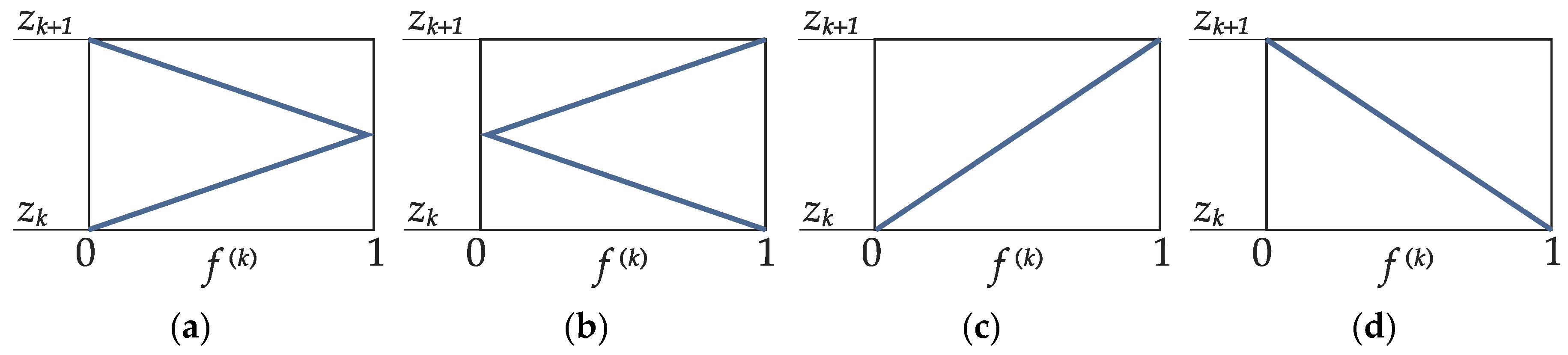
where $V_F,V_M$ are the volume fractions of the fibers and of the matrix, respectively. They are related by the following relation: $V_M=1-V_F$. In the current research, a non-uniform distribution of the fibers is defined along the plate thickness. Therefore, the volume fraction of the reinforcing fibers turns out to be a function of the thickness coordinate $V_F=V_F\left(z\right)={\tilde{V}}_F{f}^{\left(k\right)}\left(z\right)$, in which ${\tilde{V}}_F$ represents a constant value. This idea is representative of functionally graded materials. Several distributions $f^{\left(k\right)}\left(z\right)$ can be introduced toward this aim, and can be applied in each layer separately. The following functions are used in this paper:

$$f^{\left(k\right)}\left(z\right)=\{\begin{array}{l}{f}_{UD}^{\left(k\right)}\left(z\right)=1\\ f_O^{\left(k\right)}\left(z\right)=1-\frac{1}{2}\left|\frac{2\left(z-z_k\right)}{z_{k+1}-z_k}-\frac{2\left(z_{k+1}-z\right)}{z_{k+1}-z_k}\right|\\ f_X^{\left(k\right)}\left(z\right)=\frac{1}{2}\left|\frac{2\left(z-z_k\right)}{z_{k+1}-z_k}-\frac{2\left(z_{k+1}-z\right)}{z_{k+1}-z_k}\right|\\ f_V^{\left(k\right)}\left(z\right)=\frac{z-z_k}{z_{k+1}-z_k}\\ f_A^{\left(k\right)}\left(z\right)=\frac{z_{k+1}-z}{z_{k+1}-z_k}\end{array}.$$

(28)

For the sake of completeness, these functions are depicted in Figure 2.

Once the Hill’s elastic moduli (27) are computed, the engineering constants of the $k$-th fiber reinforced composite layer can be evaluated as well. The definitions shown below are required for this purpose:

$$E_{11}^{\left(k\right)}=n-\frac{l^2}{k},\hspace{1em}{E}_{22}^{\left(k\right)}=\frac{4m\left(kn-l^2\right)}{kn-l^2+mn},\hspace{1em}{\nu }_{12}^{\left(k\right)}=\frac{l}{2k},\hspace{1em}{G}_{12}^{\left(k\right)}=G_{13}^{\left(k\right)}=p,\hspace{1em}{G}_{23}^{\left(k\right)}=m.$$

(29)

It should be noted that these quantities are all functions of the thickness coordinate $z$ due to the relations (28). As a consequence, the material properties ${\overline{Q}}_{ij}^{\left(k\right)}$ defined in (23) depend also on the coordinate $z$, and the integrals in (22) have to be computed numerically. The function “trapz” embedded in MATLAB was employed toward this aim.

At this point, the Hamilton’s variational principle can be applied to obtain the equations of motion and the corresponding weak form [23]. As a result, it is possible to write the dynamic fundamental system in each element as follows:

$$\underset{\left(9\times 5\right)\times \left(9\times 5\right)}{K^{\left(e\right)}}\underset{\left(9\times 5\right)\times 1}{{\overline{u}}^{\left(e\right)}}+\underset{\left(9\times 5\right)\times \left(9\times 5\right)}{M^{\left(e\right)}}\underset{\left(9\times 5\right)\times 1}{{\ddot{\overline{u}}}^{\left(e\right)}}=0,$$

(30)

where the stiffness matrix of the element is denoted by $K^{\left(e\right)}$, whereas the mass matrix is identified by $M^{\left(e\right)}$. On the other hand, the vector ${\ddot{\overline{u}}}^{\left(e\right)}$ collects the second-order derivatives with respect to the time variable $t$ of the nodal displacements (7). By definition, the stiffness matrix $K^{\left(e\right)}$ assumes the following aspect:

$$K^{\left(e\right)}={\displaystyle \underset{x}{\int }{\displaystyle \underset{y}{\int }\underset{\left(9\times 5\right)\times 8}{B^T}\underset{8\times 8}{C}\underset{8\times \left(9\times 5\right)}{B}dxdy}}=\left[\begin{array}{ccccc}{K}_{11}& K_{12}& K_{13}& K_{14}& K_{15}\\ K_{21}& K_{22}& K_{23}& K_{24}& K_{25}\\ K_{31}& K_{32}& K_{33}& K_{34}& K_{35}\\ K_{41}& K_{42}& K_{43}& K_{44}& K_{45}\\ K_{51}& K_{52}& K_{53}& K_{54}& K_{55}\end{array}\right],$$

(31)

where the operators $K_{ij}$ of size 9 × 9 are illustrated in Appendix A. Analogously, the mass matrix $M^{\left(e\right)}$ can be written as follows:

$$M^{\left(e\right)}={\displaystyle \underset{x}{\int }{\displaystyle \underset{y}{\int }\underset{\left(9\times 5\right)\times 5}{N^T}\underset{5\times 5}{m}\underset{5\times \left(9\times 5\right)}{N}dxdy}}=\left[\begin{array}{ccccc}{M}_{11}& 0& 0& M_{14}& 0\\ 0& M_{22}& 0& 0& M_{25}\\ 0& 0& M_{33}& 0& 0\\ M_{41}& 0& 0& M_{44}& 0\\ 0& M_{52}& 0& 0& M_{55}\end{array}\right],$$

(32)

where the operators $M_{ij}$ of size 9 × 9 are also illustrated in Appendix A. The matrix $m$ instead collects the inertia terms and assumes the definition shown below:

$$m=\left[\begin{array}{ccccc}{I}_0& 0& 0& I_1& 0\\ 0& I_0& 0& 0& I_1\\ 0& 0& I_0& 0& 0\\ I_1& 0& 0& I_2& 0\\ 0& I_1& 0& 0& I_2\end{array}\right],$$

(33)

in which

$$I_i={\displaystyle \sum _{k=1}^{N_L}{\displaystyle \underset{z_k}{\overset{z_{k+1}}{\int }}{\rho }^{\left(k\right)}{z}^{i}dz}},$$

(34)

where ${\rho }^{\left(k\right)}$ is the density of the $k$-th layer. Its value can be obtained by means of the rule of mixture, combining the densities of the reinforcing fibers ${\rho }_F^{\left(k\right)}$ and of the matrix ${\rho }_M^{\left(k\right)}$:

$${\rho }^{\left(k\right)}=V_F{\rho }_F^{\left(k\right)}+V_M{\rho }_M^{\left(k\right)}.$$

(35)

Note that the density is also a function of the thickness coordinate $z$ due to the through-the-thickness variation of the volume fraction of the fibers. Therefore, the integrals in (34) have to be computed numerically as well.

2.1. Numerical Evaluation of the Fundamental Operators

It is well-known that the integrals in definitions (31) and (32) require a tool to be computed numerically. In the current research, the Gauss–Legendre rule is used. According to this approach, the infinitesimal area $dxdy$ is evaluated in the master element as follows, through the determinant of the Jacobian matrix: $dxdy=\det Jd\xi d\eta$. Consequently, the integral of a generic two-dimensional function $F\left(x,y\right)$ can be written as

$${\displaystyle \underset{x}{\int }{\displaystyle \underset{y}{\int }F\left(x,y\right)dxdy}}={\displaystyle \underset{-1}{\overset{1}{\int }}{\displaystyle \underset{-1}{\overset{1}{\int }}F\left(\xi ,\eta \right)\det Jd\xi d\eta }}.$$

(36)

At this point, the integral is converted into a weighted linear sum by introducing the roots of Legendre polynomials ${\xi }_I,{\eta }_J$ and the corresponding weighting coefficients $W_I,W_J$:

$${\displaystyle \underset{-1}{\overset{1}{\int }}{\displaystyle \underset{-1}{\overset{1}{\int }}F\left(\xi ,\eta \right)\det Jd\xi d\eta }}\approx {\displaystyle \sum _{I=1}^M{\displaystyle \sum _{J=1}^{N}F\left({\xi }_I,{\eta }_J\right){\det J|}_{{\xi }_I,{\eta }_J}{W}_I{W}_J}}.$$

(37)

The values of the roots of Legendre polynomials and the corresponding weighting coefficients used in the numerical integration are listed in

Table 1. Roots of Legendre polynomials and weighting coefficients for the numerical integration.

$N,M$	${\xi }_I,{\eta }_J$	$W_I,W_J$
2	$\pm 1/\sqrt{3}$	$1$
3	$\pm \sqrt{3/5}$	$5/9$
	$0$	$8/9$

. Recall that the full integration is performed by setting $N=M=3$. On the other hand, the reduced integration is accomplished for $N=M=2$ as far as the shear terms are concerned. In other words, the elements of the stiffness matrix which involve the mechanical properties $A_{44},A_{45},A_{55}$ are computed by means of the reduced integration. This procedure aims to avoid the shear locking problem as highlighted in the book by Reddy [14]. For the sake of completeness, the roots of Legendre polynomials are also depicted in Figure 1, for both the full and reduced integrations.

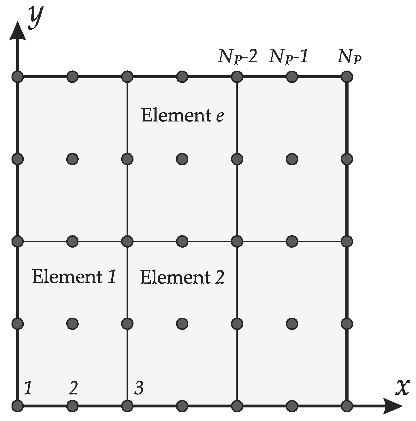
Finally, the assembly procedure is performed to enforce the $C^0$ compatibility conditions among the elements in which the reference domain is divided. In other words, the model is characterized by continuous displacements at the interfaces of the elements. The global discrete system of governing equations assumes the following aspect:

$$\underset{N_{dofs}\times N_{dofs}}{K}\underset{N_{dofs}\times 1}{u}+\underset{N_{dofs}\times N_{dofs}}{M}\underset{N_{dofs}\times 1}{\ddot{u}}=0,$$

(38)

where the number of degrees of freedom is given by $N_{dofs}=5\times N_P$, $N_P$ being the number of nodes of the discrete domain. With reference to Equation (38), $K,M$ clearly stand for the global stiffness and mass matrices, whereas $u$ is the vector of the nodal displacements of the global system defined below:

$$u={\left[\begin{array}{ccccccccccccccc}{u}_{x,1}& \cdots & u_{x,N_P}& u_{y,1}& \cdots & u_{y,N_P}& u_{z,1}& \cdots & u_{z,N_P}& {\varphi }_{x,1}& \cdots & {\varphi }_{x,N_P}& {\varphi }_{y,1}& \cdots & {\varphi }_{y,N_P}\end{array}\right]}^T,$$

(39)

in which the numbering is performed following the scheme in Figure 3. Finally, $\ddot{u}$ is the vector that collects the second-order time derivatives of the nodal displacements.

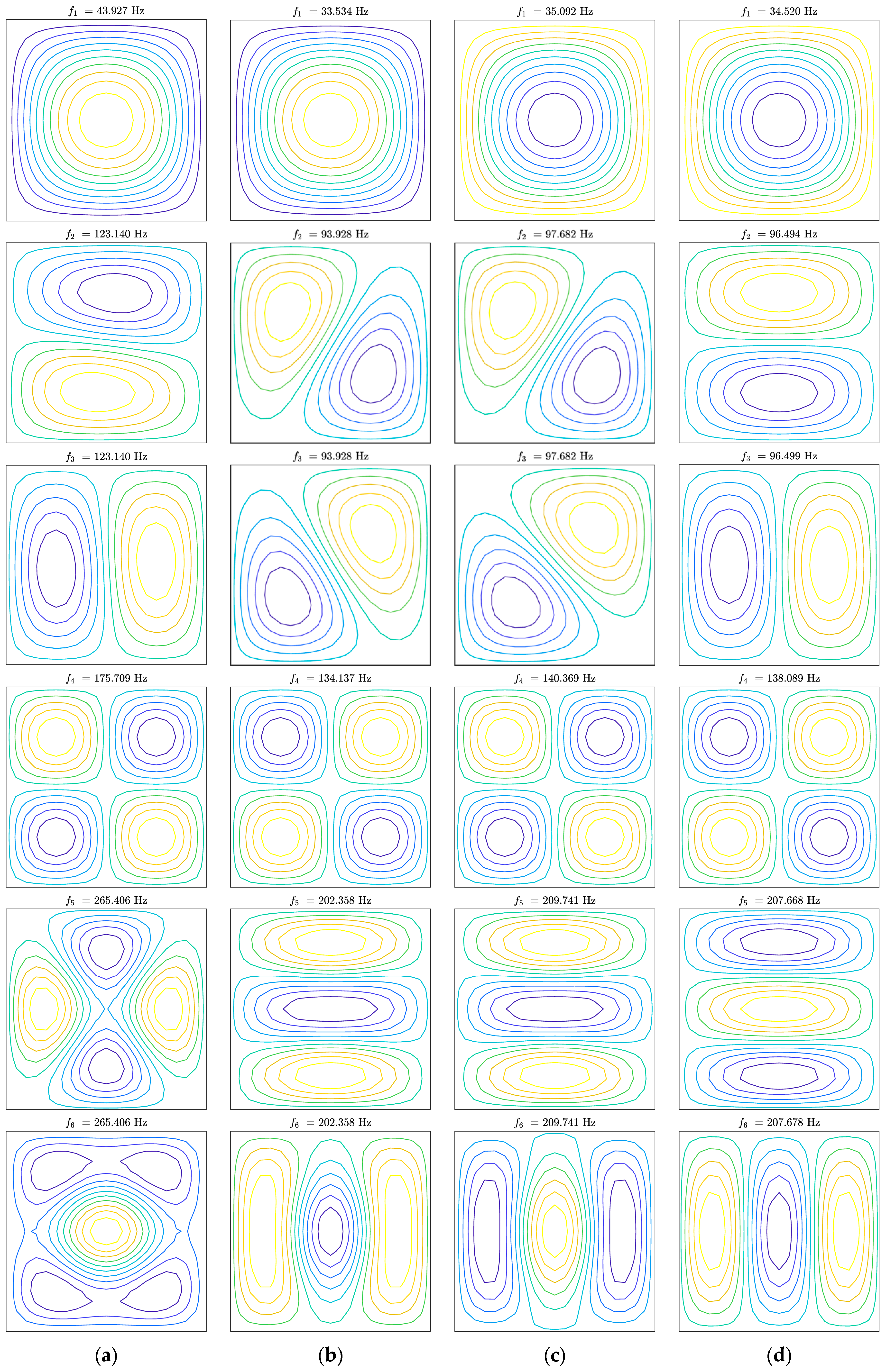
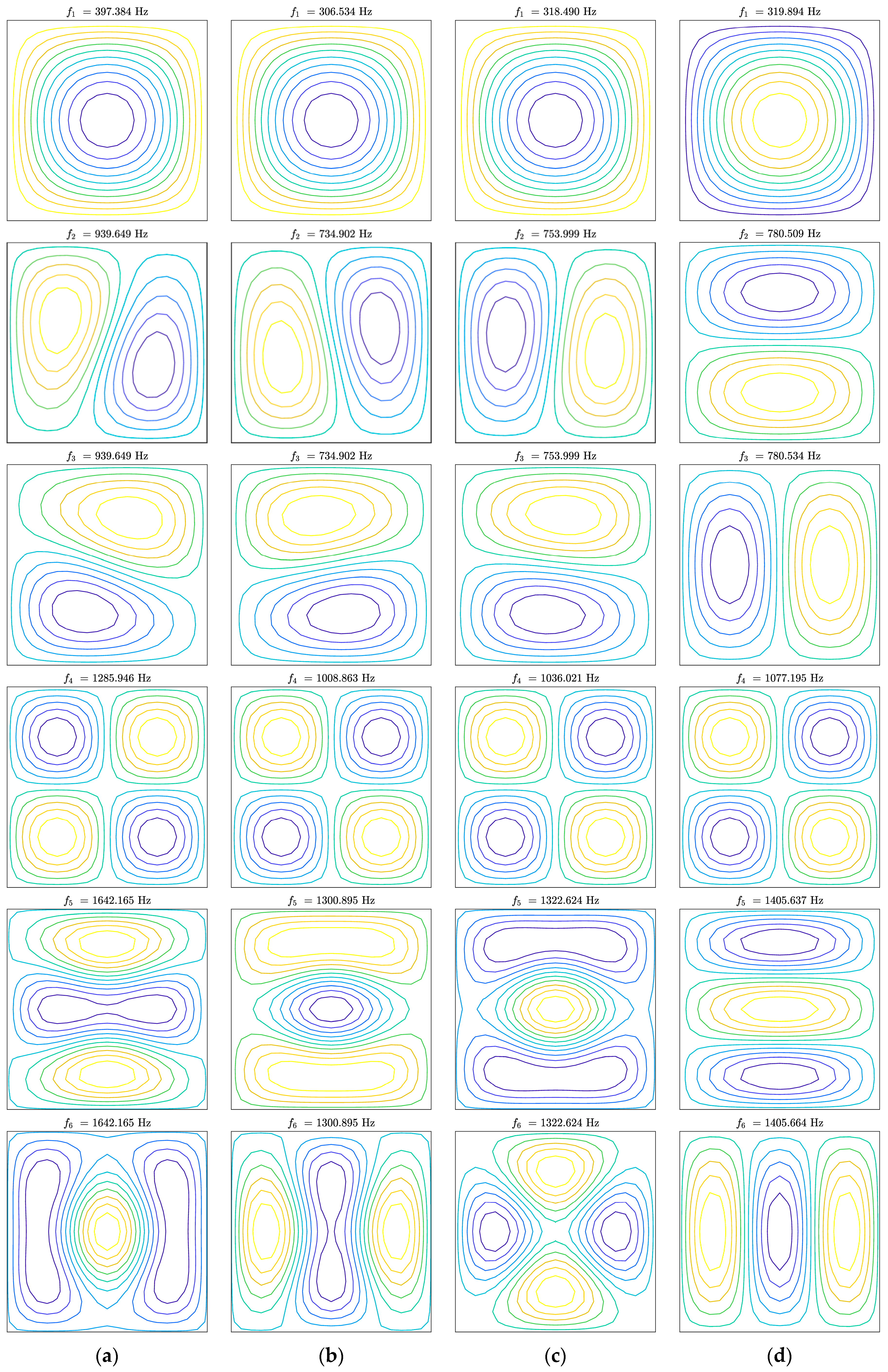
2.2. Natural Frequency Analysis

Once the discrete fundamental system (38) is defined and the proper boundary conditions are enforced, the separation of variables provide the following relation:

$$\left(K-{\omega }^{2}M\right)d=0,$$

(40)

in which $\omega$ represents the circular frequencies of the structural system, whereas the vector $d$ collects the corresponding modal amplitudes. The natural frequencies of the plate can be evaluated as $f_n=\omega /2\pi$. It can be observed that the expression (40) is a generalized eigenvalue problem. In the present research, the function “eigs” embedded in MATLAB was employed to obtain the natural frequencies and the mode shapes of the laminated composite plates.

3. Numerical Applications

The formulation illustrated in the previous section was implemented in a MATLAB code. The current approach was first validated by means of the comparison with the semi-analytical solutions provided by Reddy in his book [23], for both thin and thick simply-supported plates with an antisymmetric cross-ply layup. In these circumstances, a uniform distribution of the fiber was assumed along the plate thickness.

The convergence analysis was also performed for the sake of completeness. Subsequently, the natural frequencies of functionally graded orthotropic laminated plates are discussed. The geometry of the plates considered in the numerical applications was defined by L_x = L_y = 1 m, whereas their lamination scheme was given by $\left(0^{°}/{90}^{°}/0^{°}/{90}^{°}\right)$. The four layers were characterized by the same value of ${\tilde{V}}_F=0.6$, whereas their thickness was assumed as 2.5 × 10⁻³ m for thin plates and as 2.5 × 10⁻² m for the thick ones. The mechanical properties of the constituents (Carbon fibers and epoxy resin) are listed in

Table 2. Mechanical properties of the layer constituents.

Constituent	Young’s Moduli	Shear Moduli	Poisson’s Ratios	Density
Carbon fibers	$E_{11}^F=230\mathrm{GPa}$	$G_{12}^F=50\mathrm{GPa}$	${\nu }_{12}^F=0.20$	${\rho }^F=1800\mathrm{kg}/{\mathrm{m}}^3$
	$E_{22}^F=15\mathrm{GPa}$		${\nu }_{23}^F=0.25$
Epoxy resin	$E^M=3.27\mathrm{GPa}$	-	${\nu }^M=0.38$	${\rho }^M=1200\mathrm{kg}/{\mathrm{m}}^3$

.

3.1. Convergence and Accuracy

The convergence analysis was performed by increasing the number of discrete elements up to 256, which means 16 elements along each principal direction. The results of this test are presented in

Table 3. Convergence features of the numerical approach and comparison of the first ten natural frequencies (Hz) with the semi-analytical solutions provided by Reddy [23] for a simply-supported thin plate with a through-the-thickness uniform distribution of the reinforcing fibers. CLPT: classical laminated plate theory.

Mode	CLPT Ref. [23]	4 Elements ${\mathit{N}}_{\mathit{d}\mathit{o}\mathit{f}\mathit{s}}=125$	16 Elements ${\mathit{N}}_{\mathit{d}\mathit{o}\mathit{f}\mathit{s}}=405$	64 Elements ${\mathit{N}}_{\mathit{d}\mathit{o}\mathit{f}\mathit{s}}=1445$	256 Elements ${\mathit{N}}_{\mathit{d}\mathit{o}\mathit{f}\mathit{s}}=5445$
1	43.9262	44.4153	43.9592	43.9284	43.9265
2	123.1041	135.1515	124.3804	123.1900	123.1096
3	123.1041	135.1515	124.3804	123.1901	123.1096
4	175.6547	192.6267	177.6096	175.7865	175.6632
5	265.0021	505.8042	278.5590	265.9668	265.0653
6	265.0021	505.8084	278.5590	265.9668	265.0653
7	300.0618	533.0928	313.2389	300.9965	300.1230
8	300.0618	533.0928	313.2389	300.9965	300.1230
9	395.0350	751.5685	415.3231	396.4841	395.1299
10	465.3946	838.4999	515.4317	470.6168	465.7466

for a thin plate and in

Table 4. Convergence features of the numerical approach and comparison of the first ten natural frequencies (Hz) with the semi-analytical solutions provided by Reddy [23] for a simply-supported thick plate with a through-the-thickness uniform distribution of the reinforcing fibers. FSDT: first-order shear deformation theory.

Mode	FSDT Ref. [23]	4 Elements ${\mathit{N}}_{\mathit{d}\mathit{o}\mathit{f}\mathit{s}}=125$	16 Elements ${\mathit{N}}_{\mathit{d}\mathit{o}\mathit{f}\mathit{s}}=405$	64 Elements ${\mathit{N}}_{\mathit{d}\mathit{o}\mathit{f}\mathit{s}}=1445$	256 Elements ${\mathit{N}}_{\mathit{d}\mathit{o}\mathit{f}\mathit{s}}=5445$
1	397.3772	400.9285	397.6161	397.3928	397.3782
2	939.4637	987.3930	946.0547	939.9116	939.4924
3	939.4637	987.3930	946.0547	939.9116	939.4924
4	1285.7309	1295.8113	1293.1889	1286.2465	1285.7646
5	1640.7304	2202.4349	1687.2607	1644.1525	1640.9552
6	1640.7304	2219.9298	1687.2607	1644.1525	1640.9552
7	1869.3853	2219.9298	1905.9136	1872.1146	1869.5668
8	1869.3853	2224.7306	1905.9136	1872.1146	1869.5668
9	2313.9852	2486.7150	2349.5762	2316.8723	2314.1827
10	2372.3369	3354.9399	2442.9101	2385.5578	2373.2355

for the thicker ones, in terms of the first ten natural frequencies. A very good accuracy was obtained by using only eight finite elements per side, for both cases under consideration. In particular, the percentage error for the first mode shapes was lower than $0.4\%$ if 64 elements were used. Therefore, the formulation and the numerical approach were validated. Only the bending mode shapes were considered in the analyses.

For completeness, the convergence features of the proposed approach are presented in graphical form in Figure 4, where the relative error $e_r=f_n/f_{n,exact}-1$ was computed for increasing values of the degrees of freedom ($N_{dofs}$). The graphs are presented in logarithmic scale. It can be observed that a good convergence was reached for both thin and thick plates.

3.2. Natural Frequency Analysis of Functionally Graded Orthotropic Plates

In this section, four different through-the-thickness fiber distributions are analyzed. These four schemes, as well as the functions $f^{\left(k\right)}$ employed in each layer, are summarized in

Table 5. Definition of the through-the-thickness distribution of the reinforcing fibers.

Scheme	Layer 1	Layer 2	Layer 3	Layer 4
Scheme 1	$f_{UD}^{\left(1\right)}$	$f_{UD}^{\left(2\right)}$	$f_{UD}^{\left(3\right)}$	$f_{UD}^{\left(4\right)}$
Scheme 2	$f_O^{\left(1\right)}$	$f_O^{\left(2\right)}$	$f_O^{\left(3\right)}$	$f_O^{\left(4\right)}$
Scheme 3	$f_X^{\left(1\right)}$	$f_X^{\left(2\right)}$	$f_X^{\left(3\right)}$	$f_X^{\left(4\right)}$
Scheme 4	$f_V^{\left(1\right)}$	$f_{UD}^{\left(2\right)}$	$f_{UD}^{\left(3\right)}$	$f_A^{\left(4\right)}$

. The layers were numbered from the bottom to the top surface of the plate. As far as the mechanical and geometric features of the plates are concerned, the same values of the previous section were used. Due to the results of the convergence analyses, the plates were discretized by using ten finite elements per side. The first fourteen natural frequencies of a simply-supported thin plate for the various through-the-thickness distributions of the reinforcing fibers specified in Table 5 are presented in

Table 6. First fourteen natural frequencies (Hz) of a simply-supported thin plate for several through-the-thickness distributions of the reinforcing fibers.

Mode	Scheme 1	Scheme 2	Scheme 3	Scheme 4
1	43.9271	33.5339	35.0923	34.5204
2	123.1397	93.9281	97.6817	96.4943
3	123.1397	93.9281	97.6817	96.4994
4	175.7093	134.1367	140.3692	138.0894
5	265.4059	202.3576	209.7406	207.6677
6	265.4059	202.3576	209.7406	207.6780
7	300.4527	229.2791	239.2330	235.8151
8	300.4527	229.2791	239.2330	235.8250
9	395.6415	302.0350	316.0631	310.9587
10	467.6067	356.4637	368.9774	365.6794
11	467.6067	356.4637	368.9774	365.6944
12	494.2235	376.9847	392.0326	387.3268
13	494.2235	376.9847	392.0326	387.3477
14	565.8001	431.8446	451.1608	444.3823

, whereas

Table 7. First fourteen natural frequencies (Hz) of a simply-supported thick plate for several through-the-thickness distributions of the reinforcing fibers.

Mode	Scheme 1	Scheme 2	Scheme 3	Scheme 4
1	397.3836	306.5341	318.4900	319.8942
2	939.6493	734.9017	753.9989	780.5089
3	939.6493	734.9017	753.9989	780.5337
4	1285.9465	1008.8635	1036.0206	1077.1948
5	1642.1651	1300.8952	1322.6235	1405.6371
6	1642.1651	1300.8952	1322.6235	1405.6638
7	1870.5349	1480.8980	1510.3561	1600.6668
8	1870.5349	1480.8980	1510.3561	1600.6865
9	2315.2138	1839.1055	1872.3302	1997.7076
10	2377.9654	1899.9655	1921.4452	2077.7168
11	2377.9654	1899.9655	1921.4452	2077.7322
12	2545.0693	2031.1334	2059.3510	2219.4198
13	2545.0693	2031.1334	2059.3510	2219.4394
14	2888.3228	2306.5360	2339.2521	2523.7454

collects the same results for a simply-supported thick plate. Finally, the first six mode shapes are also depicted in graphical form. In particular, Figure 5 presents the mode shapes related to the thin plates, whereas the same results for the thick plates are shown in Figure 6. Note that the mode shapes assumed different aspects by varying the through-the-thickness distributions of the fibers in the four layers, keeping their orientation constant. Analogously, the values of natural frequencies were affected by the non-uniform distribution of the fibers along the thickness of the structures, for both thin and thick configurations.

4. Conclusions

A FE formulation was presented and implemented to investigate the natural frequencies of functionally graded orthotropic thin and thick plates with cross-ply layups. The layers of the structures were modeled as fiber-reinforced materials with orthotropic features. The fibers were characterized by a gradual variation of their volume fraction along the thickness of the plates. Toward this aim, several functions depending on the thickness coordinate were introduced. Their effects on the free vibrations were discussed. The research proved that the natural frequencies, as well as the corresponding mode shapes, were affected by the non-uniform placement of the fibers in the thickness direction. In particular, the dynamic response of laminated plates could be changed by varying the through-the-thickness distributions of the volume fraction of the reinforcing fibers, keeping the fiber orientation and the thickness of the various layers constant. The same considerations were deduced for thin and thick plates.

References

1. Kardestuncer, H.; Norrie, D.H. Finite Element Handbook; McGraw-Hill: New York, NY, USA, 1987. [Google Scholar]
2. Duncan, W.J.; Collar, A.R. A method for the solution of oscillations problems by matrices. Lond. Edinb. Dublin Philos. Mag. J. Sci. 1934, 17, 865–909. [Google Scholar] [CrossRef]
3. Duncan, W.J.; Collar, A.R. Matrices applied to the motions of damped systems. Lond. Edinb. Dublin Philos. Mag. J. Sci. 1935, 19, 197–219. [Google Scholar] [CrossRef]
4. Hrennikoff, A. Solution of Problems of Elasticity by the Frame-Work Method. ASME J. Appl. Mech. 1941, 8, A619–A715. [Google Scholar]
5. Courant, R. Variational methods for the solution of problems of equilibrium and vibration. Bull. Am. Math. Soc. 1943, 49, 1–23. [Google Scholar] [CrossRef]
6. Clough, R.W. The finite element method in plane stress analysis. In Proceedings of the 2nd A.S.C.E. Conference in Electronics Computation, Pittsburgh, PA, USA, 8–9 September 1960. [Google Scholar]
7. Melosh, R.J. Basis for derivation of matrices for the direct stiffness method. AIAA J. 1963, 1, 1631–1637. [Google Scholar]
8. Ouakka, S.; Fantuzzi, N. Trustworthiness in Modeling Unreinforced and Reinforced T-Joints with Finite Elements. Math. Comput. Appl. 2019, 24, 27. [Google Scholar] [CrossRef]
9. Uzun, B.; Civalek, Ö. Nonlocal FEM Formulation for Vibration Analysis of Nanowires on Elastic Matrix with Different Materials. Math. Comput. Appl. 2019, 24, 38. [Google Scholar] [CrossRef]
10. Oden, J.T. Finite Elements of Nonlinear Continua; McGraw-Hill: New York, NY, USA, 1972. [Google Scholar]
11. Oden, J.T.; Reddy, J.N. An Introduction to the Mathematical Theory of Finite Elements; John Wiley: New York, NY, USA, 1976. [Google Scholar]
12. Hinton, E. Numerical Methods and Software for Dynamic Analysis of Plates and Shells; Pineridge Press: Swansea, UK, 1988. [Google Scholar]
13. Zienkiewicz, O.C. The Finite Element Method; McGraw-Hill: New York, NY, USA, 1991. [Google Scholar]
14. Reddy, J.N. An Introduction to the Finite Element Method; McGraw-Hill: New York, NY, USA, 1993. [Google Scholar]
15. Onate, E. Calculo de Estruturas por el Metodo de Elementos Finitos; CIMNE: Barcelona, Spain, 1995. [Google Scholar]
16. Hughes, T.J.R. The Finite Element Method—Linear Static and Dynamic Finite Element Analysis; Dover Publications: New York, NY, USA, 2000. [Google Scholar]
17. Ferreira, A.J.M. MATLAB Codes for Finite Element Analysis; Springer: New York, NY, USA, 2008. [Google Scholar]
18. Dezi, L.; Menditto, G.; Tarantino, A.M. Homogeneous structures subjected to successive structural system changes. J. Eng. Mech. ASCE 1990, 116, 1723–1732. [Google Scholar] [CrossRef]
19. Dezi, L.; Tarantino, A.M. Time dependent analysis of concrete structures with variable structural system. ACI Mater. J. 1991, 88, 320–324. [Google Scholar]
20. Dezi, L.; Menditto, G.; Tarantino, A.M. Viscoelastic heterogeneous structures with variable structural system. J. Eng. Mech. ASCE 1993, 119, 238–250. [Google Scholar] [CrossRef]
21. Dezi, L.; Tarantino, A.M. Creep in continuous composite beams. Part I: Theoretical treatment. J. Struct. Eng. ASCE 1993, 119, 2095–2111. [Google Scholar] [CrossRef]
22. Reddy, J.N.; Miravete, A. Practical Analysis of Composite Laminates; CRC Press: Boca Raton, FL, USA, 1995. [Google Scholar]
23. Reddy, J.N. Mechanics of Laminated Composite Plates and Shells—Theory and Analysis, 2nd ed.; CRC Press: Boca Raton, FL, USA, 2004. [Google Scholar]
24. Tornabene, F.; Bacciocchi, M. Anisotropic Doubly-Curved Shells. Higher-Order Strong and Weak Formulations for Arbitrarily Shaped Shell Structures; Esculapio: Bologna, Italy, 2018. [Google Scholar]
25. Vinson, J.R. The Behavior of Shells Composed of Isotropic and Composite Materials; Springer: New York, NY, USA, 1993. [Google Scholar]
26. Jones, R.M. Mechanics of Composite Materials, 2nd ed.; Taylor & Francis: Philadelphia, PA, USA, 1999. [Google Scholar]
27. Christensen, R.M. Mechanics of Composite Materials; Dover Publications: New York, NY, USA, 2005. [Google Scholar]
28. Barbero, E.J. Introduction to Composite Materials Design; CRC Press: Boca Raton, FL, USA, 2011. [Google Scholar]
29. Chamis, C.C.; Sendeckyj, G.P. Critique on Theories Predicting Thermoelastic Properties of Fibrous Composites. J. Compos. Mater. 1968, 2, 332–358. [Google Scholar] [CrossRef]
30. Halpin, J.C. Effects of Environmental Factors on Composite Materials. Available online: http://citeseerx.ist.psu.edu/viewdoc/download?doi=10.1.1.844.575&rep=rep1&type=pdf (accessed on 18 May 2019).
31. Tsai, S.W. Structural Behavior of Composite Materials; NASA: Washington, DC, USA, 1964.
32. Tsai, S.W. Strength Characteristics of Composite Materials; NASA: Washington, DC, USA, 1965.
33. Hill, R. Theory of Mechanical Properties of Fibre-Strengthened Materials: I. Elastic Behavior. J. Mech. Phys. Solids 1964, 12, 199–212. [Google Scholar] [CrossRef]
34. Hill, R. Theory of Mechanical Properties of Fibre-Strengthened Materials: II. Inelastic Behavior. J. Mech. Phys. Solids 1964, 12, 213–218. [Google Scholar] [CrossRef]
35. Tornabene, F.; Bacciocchi, M.; Fantuzzi, N.; Reddy, J.N. Multiscale Approach for Three-Phase CNT/Polymer/ Fiber Laminated Nanocomposite Structures. Polym. Compos. 2019, 40, E102–E126. [Google Scholar] [CrossRef]
36. Reddy, J.N.; Chin, C.D. Thermomechanical Analysis of Functionally Graded Cylinders and Plates. J. Therm. Stresses 1998, 21, 593–626. [Google Scholar] [CrossRef]
37. Reddy, J.N. Analysis of functionally graded plates. Int. J. Numer. Methods Eng. 2000, 47, 663–684. [Google Scholar] [CrossRef]
38. Reddy, J.N. Microstructure-dependent couple stress theories of functionally graded beams. J. Mech. Phys. Solids 2011, 59, 2382–2399. [Google Scholar] [CrossRef]
39. Reddy, J.N.; Kim, J. A nonlinear modified couple stress-based third-order theory of functionally graded plates. Compos. Struct. 2012, 94, 1128–1143. [Google Scholar] [CrossRef]
40. Kim, J.; Reddy, J.N. A general third-order theory of functionally graded plates with modified couple stress effect and the von Kármán nonlinearity: Theory and finite element analysis. Acta Mech. 2015, 226, 2973–2998. [Google Scholar] [CrossRef]
41. Kim, J.; Reddy, J.N. Modeling of functionally graded smart plates with gradient elasticity effects. Mech. Adv. Mater. Struct. 2017, 24, 437–447. [Google Scholar] [CrossRef]
42. Kim, J.; Zur, K.K.; Reddy, J.N. Bending, free vibration, and buckling of modified couples stress-based functionally graded porous micro-plates. Compos. Struct. 2019, 209, 879–888. [Google Scholar] [CrossRef]
43. Gutierrez Rivera, M.; Reddy, J.N. Stress analysis of functionally graded shells using a 7-parameter shell element. Mech. Res. Commun. 2016, 78, 60–70. [Google Scholar] [CrossRef]
44. Lanc, D.; Vo, T.P.; Turkalj, G.; Lee, J. Buckling analysis of thin-walled functionally graded sandwich box beams. Thin Wall. Struct. 2015, 86, 148–156. [Google Scholar] [CrossRef]
45. Lanc, D.; Turkalj, G.; Vo, T.; Brnic, J. Nonlinear buckling behaviours of thin-walled functionally graded open section beams. Compos. Struct. 2016, 152, 829–839. [Google Scholar] [CrossRef]
46. Sofiyev, A.H.; Kuruoglu, N. Dynamic instability of three-layered cylindrical shells containing an FGM interlayer. Thin Wall. Struct. 2015, 93, 10–21. [Google Scholar] [CrossRef]
47. Alibeigloo, A. Thermo elasticity solution of sandwich circular plate with functionally graded core using generalized differential quadrature method. Compos. Struct. 2016, 136, 229–240. [Google Scholar] [CrossRef]
48. Tornabene, F. Free Vibration Analysis of Functionally Graded Conical, Cylindrical Shell and Annular Plate Structures with a Four-parameter Power-Law Distribution. Comput. Method. Appl. Mech. Eng. 2009, 198, 2911–2935. [Google Scholar] [CrossRef]
49. Tornabene, F.; Viola, E. Free Vibration Analysis of Functionally Graded Panels and Shells of Revolution. Meccanica 2009, 44, 255–281. [Google Scholar] [CrossRef]
50. Tornabene, F.; Fantuzzi, N.; Viola, E.; Batra, R.C. Stress and strain recovery for functionally graded free-form and doubly-curved sandwich shells using higher-order equivalent single layer theory. Compos. Struct. 2015, 119, 67–89. [Google Scholar] [CrossRef]
51. Mercan, K.; Baltacıoglu, A.K.; Civalek, Ö. Free vibration of laminated and FGM/CNT composites annular thick plates with shear deformation by discrete singular convolution method. Compos. Struct. 2018, 186, 139–153. [Google Scholar] [CrossRef]
52. Civalek, Ö.; Baltacıoglu, A.K. Free vibration analysis of laminated and FGM composite annular sector plates. Compos. Part B Eng. 2019, 157, 182–194. [Google Scholar] [CrossRef]
53. Mróz, Z. Optimal design of structures of composite materials. Int. J. Solids Struct. 1970, 6, 859–870. [Google Scholar] [CrossRef]
54. Bert, C.W. Optimal design of a composite-material plate to maximize its fundamental frequency. J. Sound Vib. 1977, 50, 229–237. [Google Scholar] [CrossRef]
55. Bruyneel, M. A general and effective approach for the optimal design of fiber reinforced composite structures. Compos. Sci. Technol. 2006, 66, 1303–1314. [Google Scholar] [CrossRef]
56. Pelletier, J.L.; Vel, S.S. Multi-objective optimization of fiber reinforced composite laminates for strength, stiffness and minimal mass. Comput. Struct. 2006, 84, 2065–2080. [Google Scholar] [CrossRef]
57. Dong, C.; Davies, I.J. Optimal design for the flexural behaviour of glass and carbon fibre reinforced polymer hybrid composites. Mater. Design. 2012, 37, 450–457. [Google Scholar] [CrossRef]
58. Ganguli, R. Optimal design of composite structures: a historical review. J. Indian I. Sci. 2013, 93, 557–570. [Google Scholar]
59. Ke, L.-L.; Yang, J.; Kitipornchai, S. Nonlinear free vibration of functionally graded carbon nanotube-reinforced composite beams. Compos. Struct. 2010, 92, 676–683. [Google Scholar] [CrossRef]
60. Shen, H.-S. Thermal buckling and postbuckling behavior of functionally graded carbon nanotube-reinforced composite cylindrical shells. Compos. Part B Eng. 2012, 43, 1030–1038. [Google Scholar] [CrossRef]
61. Zhang, L.W.; Lei, Z.X.; Liew, K.M.; Yu, J.L. Static and dynamic of carbon nanotube reinforced functionally graded cylindrical panels. Compos. Struct. 2014, 111, 205–212. [Google Scholar] [CrossRef]
62. Liew, K.M.; Lei, Z.X.; Zhang, L.W. Mechanical analysis of functionally graded carbon nanotube reinforced composites: A review. Compos. Struct. 2015, 120, 90–97. [Google Scholar] [CrossRef]
63. Alibeigloo, A. Elasticity solution of functionally graded carbon nanotube-reinforced composite cylindrical panel subjected to thermo mechanical load. Compos. Part B Eng. 2016, 87, 214–226. [Google Scholar] [CrossRef]
64. Civalek, Ö. Free vibration of carbon nanotubes reinforced (CNTR) and functionally graded shells and plates based on FSDT via discrete singular convolution method. Compos. Part B Eng. 2017, 111, 45–59. [Google Scholar] [CrossRef]
65. Thang, P.T.; Nguyen, T.-T.; Lee, J. A new approach for nonlinear buckling analysis of imperfect functionally graded carbon nanotube-reinforced composite plates. Compos. Part B Eng. 2017, 127, 166–174. [Google Scholar] [CrossRef]
66. Zhao, J.; Choe, K.; Shuai, C.; Wang, A.; Wang, Q. Free vibration analysis of functionally graded carbon nanotube reinforced composite truncated conical panels with general boundary conditions. Compos. Part B Eng. 2019, 160, 225–240. [Google Scholar] [CrossRef]
67. Civalek, Ö.; Baltacıoglu, A.K. Vibration analysis of circular cylindrical panels with CNT reinforced and FGM composites. Compos. Struct. 2018, 202, 374–388. [Google Scholar]
68. Civalek, Ö.; Baltacıoglu, A.K. Vibration of carbon nanotube reinforced composite (CNTRC) annular sector plates by discrete singular convolution method. Compos. Struct. 2018, 203, 458–465. [Google Scholar] [CrossRef]
69. Bacciocchi, M.; Tarantino, A.M. Time-dependent behavior of viscoelastic three-phase composite plates reinforced by Carbon nanotubes. Compos. Struct. 2019, 216, 20–31. [Google Scholar] [CrossRef]
70. Fantuzzi, N.; Tornabene, F.; Bacciocchi, M.; Neves, A.M.A.; Ferreira, A.J.M. Stability and accuracy of three Fourier expansion-based strong form finite elements for the free vibration analysis of laminated composite plates. Int. J. Numer. Methods Eng. 2017, 111, 354–382. [Google Scholar] [CrossRef]
71. Tornabene, F.; Fantuzzi, N.; Bacciocchi, M. On the mechanics of laminated doubly-curved shells subjected to point and line loads. Int. J. Eng. Sci. 2016, 109, 115–164. [Google Scholar] [CrossRef]
Figure 1. Nine-node quadratic Lagrange rectangular element.
Mca 24 00052 g001
Figure 2. Through-the-thickness variation of f ( k ) : (a) f O ( k ) ; (b) f X ( k ) ; (c) f V ( k ) ; (d) f A ( k ) .
Mca 24 00052 g002
Figure 3. Example of a discrete domain and node numbering.
Mca 24 00052 g003
Figure 4. Convergence graphs for thin (CLPT) and thick (FSDT) laminated plates in terms of natural frequencies: (a) first frequency; (b) second frequency; (c) third frequency; (d) fourth frequency; (e) fifth frequency; (f) sixth frequency.
Mca 24 00052 g004
Figure 5. First six mode shapes for a simply-supported laminated thin plate with different fiber distributions: (a) Scheme 1 (uniform); (b) Scheme 2; (c) Scheme 3; (d) Scheme 4.
Mca 24 00052 g005
Figure 6. First six mode shapes for a simply-supported laminated thick plate with different fiber distributions: (a) Scheme 1 (uniform); (b) Scheme 2; (c) Scheme 3; (d) Scheme 4.
Mca 24 00052 g006