Relaxed Projection Methods with Self-Adaptive Step Size for Solving Variational Inequality and Fixed Point Problems for an Infinite Family of Multivalued Relatively Nonexpansive Mappings in Banach Spaces

Abstract

In each iteration, the projection methods require computing at least one projection onto the closed convex set. However, projections onto a general closed convex set are not easily executed, a fact that might affect the efficiency and applicability of the projection methods. To overcome this drawback, we propose two iterative methods with self-adaptive step size that combines the Halpern method with a relaxed projection method for approximating a common solution of variational inequality and fixed point problems for an infinite family of multivalued relatively nonexpansive mappings in the setting of Banach spaces. The core of our algorithms is to replace every projection onto the closed convex set with a projection onto some half-space and this guarantees the easy implementation of our proposed methods. Moreover, the step size of each algorithm is self-adaptive. We prove strong convergence theorems without the knowledge of the Lipschitz constant of the monotone operator and we apply our results to finding a common solution of constrained convex minimization and fixed point problems in Banach spaces. Finally, we present some numerical examples in order to demonstrate the efficiency of our algorithms in comparison with some recent iterative methods.

1. Introduction

Let E be a real Banach space with norm $\left|\right|·\left|\right|,$ and $E^{*}$ be the dual of $E.$ For $x\in E$ and $f\in E^{*},$ let $\langle x,f\rangle$ be the value of f at $x.$ Suppose that C is a nonempty, closed, and convex subset of $E.$ The Variational Inequality Problem (VIP) that is associated with C and A is formulated, as follows: find a point $x^{*}\in C$, such that

$$\langle x-x^{*},A{x}^{*}\rangle \ge 0,\forall x\in C,$$

(1)

where $A:E\to E^{*}$ is a single-valued mapping. We denote the solution set of VIP (1) by $VI(C,A).$

Let C be a nonempty, closed, and convex subset of a real Hilbert space $H.$ A mapping $P_C$ is said to be the metric projection of H onto C if, for all $x\in H,$ there exists a unique nearest point in $C,$ denoted by $P_{C}x,$ such that

$$\left|\right|x-P_{C}x\left|\right|\le \left|\right|x-y\left|\right|,\forall y\in C.$$

Variational inequality was first introduced independently by Fichera [1] and Stampacchia [2]. The VIP is a useful mathematical model that unifies many important concepts in applied mathematics, such as necessary optimality conditions, complementarity problems, network equilibrium problems, and systems of nonlinear equations (see [3,4,5,6,7]). Many authors have proposed and analysed several iterative algorithms for solving the VIP (1) and related optimization problems, see [8,9,10,11,12,13,14,15,16,17,18,19,20,21] and references therein. One of the most famous of these methods is the extragradient method (EgM) proposed by Korpelevich [22], which is presented in Algorithm 1, as follows:

Algorithm 1: Extragradient Method (EgM)

$$\left\{\begin{array}{c}{x}_0\in C,\hfill \\ y_n=P_C(x_n-\lambda A{x}_n),\hfill \\ x_{n+1}=P_C(x_n-\lambda A{y}_n),\hfill \end{array}\right.$$

where $C\subseteq {\mathbb{R}}^n,A:C\to {\mathbb{R}}^n$ is a monotone and $L-$Lipschitz continuous operator with $\lambda \in (0,\frac{1}{L}).$ If the solution set $VI(C,A)$ is nonempty, then the sequence $\left\{x_n\right\}$ generated by EgM converges to an element in $VI(C,A).$ The EgM was further extended to infinite dimensional spaces by many authors; see, for instance, [11,23,24]. Observe that the EgM involves two projections onto the closed convex set C and two evaluations of A per iteration. Computing projection onto an arbitrary closed convex set is a difficult task, a drawback that may affect the efficiency of the EgM, as mentioned in [25]. Hence, a major improvement on the EgM is to minimize the number of evaluations of $P_C$ per iteration. Censor et al. [25] initiated an attempt in this direction, modifying the EgM by replacing the second projection with a projection onto a half-space. This new method only involves one projection onto C and it is called the subgradient extragradient method (SEgM). The $SEgM$ algorithm is given in Algorithm 2, as follows:

Algorithm 2: Subgradient Extragradient Method (SEgM)

$$\left\{\begin{array}{c}{x}_0\in H,\hfill \\ y_n=P_C(x_n-\lambda A{x}_n),\hfill \\ Q_n=\{z\in H:\langle x_n-\lambda A{x}_n-y_n,z-y_n\rangle \le 0\},\hfill \\ x_{n+1}=P_{Q_n}(x_n-\lambda A{y}_n).\hfill \end{array}\right.$$

where H is an Hilbert space.

Censor et al. [25] showed that if the solution set $VI(C,A)$ is nonempty, the sequence $\left\{x_n\right\}$ generated by $SEgM$ converges weakly to an element $p\in VI(C,A)$, where $p={\lim }_{n\to \infty }{P}_{VI(C,A)}\left(x_n\right).$

Bauschke and Combettes [26] pointed out that, in solving optimization problems, strong convergence of iterative schemes are more desirable than their weak convergence counterparts. Hence, the need to develop algorithms that generate strong convergence sequence.

Let $S:E\to E$ be a nonlinear mapping, a point $x^{*}\in E$ is called a fixed point of S if $S{x}^{*}=x^{*}$. We denote, by $F\left(S\right)$, the set of all fixed points of $S,$ i.e.,

$$F\left(S\right)=\{x^{*}\in E:S{x}^{*}=x^{*}\}.$$

If S is a multivalued mapping, i.e., $S:E\to 2^E,$ then $x^{*}\in E$ is called a fixed point of S if

$$x^{*}\in S{x}^{*}.$$

Here, we consider the fixed point problem for an infinite family of multivalued relatively nonexpansive mappings. The fixed point theory for multivalued mappings can be utilized in various areas, such as game theory, control theory, mathematical economics, and differential inclusion (see [13,27,28] and the references therein). The existence of common fixed points for a family of mappings has been considered by many authors (see [13,28,29,30] and the references therein). Many optimization problems can be formulated as finding a point in the intersection of the fixed point sets of a family of nonlinear mappings. For instance, the well-known convex feasibility problem reduces to finding a point in the intersection of the fixed point sets of a family of nonexpansive mappings (see [31,32]). The problem of finding an optimal point that minimizes a given cost function over the common set of fixed points of a family of nonlinear mappings is of wide interdisciplinary interest and practical importance (see [33,34]). A simple algorithmic solution to the problem of minimizing a quadratic function over the common set of fixed points of a family of nonexpansive mappings is of extreme value in many applications including set theoretic signal estimation (see [34,35]).

In this article, we are interested in studying the problem of finding a common solution of both the VIP (1) and the common fixed point problem for multivalued mappings. The motivation for studying such problems lies in its potential application to mathematical models whose constraints can be expressed as fixed point problem and VIP. This happens, in particular, in practical problems, such as signal processing, network resource allocation, and image recovery. A scenario is in network bandwidth allocation problem for two services in a heterogeneous wireless access networks in which the bandwidth of the services are mathematically related (see, for instance, [36,37,38,39] and the references therein).

Observe that all of the above results about the extragradient method or subgradient extragradient method are all confined in Hilbert spaces. However, many important problems related to practical problems are generally defined in Banach spaces. For instance, Zhang et al. [40] pointed out that in machine learning, Banach spaces possess much richer geometric structures, which are potentially useful for developing learning algorithms. This is due to the fact that any two Hilbert spaces over $\mathbb{C}$ of the same dimension are isometrically isomorphic. Der and Lee [41] also pointed out that most data in machine learning do not come with any natural notion distance that can be induced from an inner-product. Zhang et al. [40] further argued that most data come with intrinsic structures that make them impossible to be embedded into a Hilbert space. Hence, it is more desirable to propose an iterative algorithm for finding a solution of VIP (1) in Banach spaces.

Very recently, Liu [42] extended the subgradient extragradient method from Hilbert spaces into Banach spaces and proposed the following strong convergence theorem.

Theorem 1.

Let E be a two-uniformly convex and uniformly smooth Banach space with the two-uniformly convexity constant $c_1$ and C be a nonempty closed convex subset of $E.$ Let $S:E\to E$ be a relatively nonexpansive mapping and $A:E\to E^{*}$ a monotone and L-Lipschitz mapping on C with $L>0.$ Let $\left\{{\lambda }_n\right\}$ be a real number sequence satisfying $0<{\inf }_{n\ge 1}{\lambda }_n\le {\sup }_{n\ge 1}{\lambda }_n<\frac{c_1}{L}.$ Suppose that $VI(C,A)\bigcap F\left(S\right)$ is nonempty. Let $\left\{x_n\right\}\subset E$ be a sequence generated by Algorithm 3, as follows:

Algorithm 3:

$$\left\{\begin{array}{c}{x}_0\in E,\hfill \\ y_n={\Pi }_C{J}^{-1}(J{x}_n-{\lambda }_{n}A\left(x_n\right)),\hfill \\ T_n=\{w\in E:\langle w-y_n,J{x}_n-{\lambda }_{n}A\left(x_n\right)-J{y}_n\rangle \le 0\},\hfill \\ w_n={\Pi }_{T_n}{J}^{-1}(J{x}_n-{\lambda }_{n}A\left(y_n\right)),\hfill \\ z_n=J^{-1}({\alpha }_{n}J{x}_0+(1-{\alpha }_n)J{w}_n),\hfill \\ x_{n+1}=J^{-1}({\beta }_{n}J{x}_n+(1-{\beta }_n)JS{z}_n),\hfill \end{array}\right.$$

where $\left\{{\beta }_n\right\}\subset [a,b]\subset [0,1]$ for some $a,b\in (0,1),\left\{{\alpha }_n\right\}\subset (0,1)$ with ${\lim }_{n\to \infty }{\alpha }_n=0$ and ${\sum }_{n=1}^{\infty }{\alpha }_n=\infty .$ Subsequently, $x_n\to {\Pi }_{VI(C,A)\bigcap F\left(S\right)}{x}_0.$

We notice that Algorithm 3 has one projection made onto the closed convex set $C.$ As earlier pointed out, computing projection onto an arbitrary closed convex set is a difficult task. Another shortcoming of Algorithm 3, the EgM and SEgM, is that the step size is defined by a constant (or a sequence) which is dependent on the Lipschitz constant of the monotone operator. The Lipschitz constant is typically assumed to be known, or at least estimated prior. However, in many cases, this parameter is unknown or difficult to estimate. Moreover, the step size that is defined by the constant is often very small and slows down the convergence rate. In practice, a larger step size can often be used and yields better numerical results. To overcome these drawbacks, in this article, motivated by the cited works and the ongoing research in this area, we propose some relaxed subgradient extragdient methods with self-adaptive step size for approximating a common solution of variational inequality and fixed point problems for an infinite family of relatively nonexpansive mappings in the setting of Banach spaces. In our algorithms, the two projections are made onto some half-space, which guarantees the easy implementation of the proposed methods. Moreover, the step size can be selected adaptively. We prove strong convergence theorems without the knowledge of the Lipschitz constant of the monotone operator and we apply our results to finding a common solution of constrained convex minimization and fixed point problems in Banach spaces. Finally, we present some numerical examples to demonstrate the efficiency of our algorithms.

2. Preliminaries

In what follows, we let $\mathbb{N}$ and $\mathbb{R}$ be the set of positive integers and real numbers, respectively. Let E be a Banach space, $E^{*}$ be the dual space of $E,$ and let $\langle ·,·\rangle$ denote the duality pairing of E and $E^{*}.$ When $\left\{x_n\right\}$ is a sequence in $E,$ we denote the strong convergence of $\left\{x_n\right\}$ to $x\in E$ by $x_n\to x$ and the weak convergence by $x_n\rightharpoonup x.$ An element $z\in E$ is called a weak cluster point of $\left\{x_n\right\}$ if there exists a subsequence $\left\{x_{n_j}\right\}$ of $\left\{x_n\right\}$ converging weakly to $z.$ We write ${\omega }_w\left(x_n\right)$ to indicate the set of all weak cluster points of $\left\{x_n\right\}.$

Next, we present some definitions and results that are employed in our subsequent analysis.

Definition 1.

A function $f:E\to \mathbb{R}$ is said to be weakly lower semicontinuous (w-lsc) at $x\in E,$ if

$$f\left(x\right)\le \underset{n\to \infty }{\lim \inf }f\left(x_n\right)$$

holds for an arbitrary sequence ${\left\{x_n\right\}}_{n=0}^{\infty }$ in E satisfying $x_n\rightharpoonup x.$

Let $g:E\to \mathbb{R}$ be a function. The subdifferential of g at x is defined by

$$\partial g\left(x\right)=\{w\in E^{*}:g\left(y\right)\ge g\left(x\right)+\langle y-x,w\rangle ,\forall y\in E\}.$$

If $\partial g\left(x\right)\ne \varnothing ,$ then we say that g is subdifferentiable at $x.$

Definition 2.

An operator$A:E\to E^{*}$is said to be

(i) 

monotone if

$$\langle x-y,Ax-Ay\rangle \ge 0,\forall x,y\in E;$$

(ii) 

α-inverse-strongly-monotone if there exists a positive real number α, such that

$$\langle x-y,Ax-Ay\rangle \ge \alpha \left|\right|Ax-{Ay\left|\right|}^2,\forall x,y\in E;$$

(iii) 

L-Lipschitz continuous if there exists a constant $L>0$ such that

$$\left|\right|Ax-Ay\left|\right|\le L\left|\right|x-y\left|\right|,\forall x,y\in E.$$

Clearly, an α-inverse-strongly-monotone mapping is monotone and $\frac{1}{\alpha }$-Lipschitz continuous. However, the converse is not always true.

A Banach space E is said to be strictly convex, if for all $x,y\in E$, such that $\left|\right|x\left|\right|=\left|\right|y\left|\right|=1$ and $x\ne y$ implies $\left|\right|(x+y)/2\left|\right|<1.$ E is said to be uniformly convex, if for each $\epsilon \in (0,2],$ there exists $\delta >0$ such that for all $x,y\in E,\left|\right|x\left|\right|=\left|\right|y\left|\right|=1$ and $\left|\right|x-y\left|\right|\ge \epsilon$ implies $\left|\right|(x+y)/2\left|\right|<1-\delta .$ It is well known that a uniformly convex Banach space is strictly convex and reflexive. The modulus of convexity of E is defined as

$${\delta }_E\left(\epsilon \right)=\inf \left\{1-\parallel \frac{x+y}{2}\parallel :x,y\in E,\left|\right|x\left|\right|=\left|\right|y\left|\right|=1,\left|\right|x-y\left|\right|\ge \epsilon \right\}.$$

Subsequently, the Banach space E is uniformly convex if and only if ${\delta }_E\left(\epsilon \right)>0$ for all $\epsilon \in (0,2].$ In particular, let H be a real Hilbert space, then ${\delta }_H\left(\epsilon \right)=1-\sqrt{1-{(\epsilon /2)}^2}.$ E is said to be p-uniformly convex if there exists a constant $c>0$ such that ${\delta }_E\left(\epsilon \right)>c{\epsilon }^p$ for all $\epsilon \in [0,2]$ with $p\ge 2.$ It is easy to see that a p-uniformly convex Banach space is uniformly convex. In particular, a Hilbert space is two-uniformly convex.

A Banach space E is said to be smooth, if the limit ${\lim }_{t\to 0}\left(\right||x+ty\left|\right|-\left|\right|x\left|\right|)/t$ exists for all $x,y\in S_E,$ where $S_E=\{x\in E:|\left|x\right||=1\}.$ Moreover, if this limit is attained uniformly for $x,y\in S_E,$ then E is said to be uniformly smooth. It is obvious that a uniformly smooth space is smooth. In particular, a Hilbert space is uniformly smooth.

For $p>1,$ the generalized duality mapping $J_p:E\to 2^{E^{*}}$ is defined, as follows:

$$J_{p}x=\{x^{*}\in E^{*}:\langle x,x^{*}\rangle ={\left|\right|x\left|\right|}^p,\left|\right|x^{*}\left|\right|={\left|\right|x\left|\right|}^{p-1}\}\forall x\in E.$$

In particular, $J=J_2$ is called the normalized duality mapping. If $E=H,$ where H is a real Hilbert space, then $J=I.$ The normalized duality mapping J has the following properties (see [43]):

(1)

if E is smooth, then J is single-valued;

(2)

if E is strictly convex, then J is one-to-one and strictly monotone;

(3)

if E is reflexive, then J is surjective; and,

(4)

if E is uniformly smooth, then J is uniformly norm-to-norm continuous on each bounded subset of $E.$

Let E be a smooth Banach space. The Lyapunov functional $\varphi :E\times E\to \mathbb{R}$ (see [44]) is defined by

$$\varphi (x,y)={\left|\right|x\left|\right|}^2-2\langle x,Jy\rangle +{\left|\right|y\left|\right|}^2\forall x,y\in E.$$

From the definition, it is easy to see that $\varphi (x,x)=0$ for every $x\in E.$ If E is strictly convex, then $\varphi (x,y)=0⟺x=y.$ If E is a Hilbert space, it is easy to see that $\varphi (x,y)=\left|\right|x-{y\left|\right|}^2$ for all $x,y\in E.$ Moreover, for every $x,y,z\in E$ and $\alpha \in (0,1),$ the Lyapunov functional $\varphi$ satisfies the following properties:

(P1)

$0\le \left(\right|\left|x\right||-{\left|\right|y\left|\right|)}^2\le \varphi (x,y)\le \left(\right|\left|x\right||+{\left|\right|y\left|\right|)}^2;$

(P2)

$\varphi (x,J^{-1}(\alpha Jz+(1-\alpha )Jy))\le \alpha \varphi (x,z)+(1-\alpha )\varphi (x,y);$

(P3)

$\varphi (x,y)=\varphi (x,z)+\varphi (z,y)+2\langle z-x,Jy-Jz\rangle ;$

(P4)

$\varphi (x,y)\le 2\langle y-x,Jy-Jx\rangle ;$

(P5)

$\varphi (x,y)=\langle x,Jx-Jy\rangle +\langle y-x,Jy\rangle \le \left|\right|x\left|\right|\left|\right|Jx-Jy\left|\right|+\left|\right|y-x\left|\right|\left|\right|y\left|\right|.$

Next, we define the functional $V:E\times E^{*}\to [0,+\infty )$ by

$$V(x,x^{*})={\left|\right|x\left|\right|}^2-2\langle x,x^{*}\rangle +\left|\right|x^{*}{\left|\right|}^2\forall x\in E,x^{*}\in E^{*}.$$

(2)

It can be deduced from (2) that V is non-negative and

$$V(x,x^{*})=\varphi (x,J^{-1}\left(x^{*}\right)).$$

We have the following result in a reflexive strictly convex and smooth Banach space.

Lemma 1.

([45]) Let E be a reflexive strictly convex and smooth Banach space with $E^{*}$ as its dual. Subsequently,

$$V(x,x^{*})+2\langle J^{-1}{x}^{*}-x,y^{*}\rangle \le V(x,x^{*}+y^{*}),$$

for all $x\in E$ and $x^{*},y^{*}\in E^{*}.$

Definition 3.

Let C be a nonempty closed convex subset of a real Banach space $E.$ A point $p\in C$ is called an asymptotic fixed point (see [46]) of T if C contains a sequence $\left\{x_n\right\}$ which converges weakly to p, such that ${\lim }_{n\to \infty }\left|\right|x_n-T{x}_n\left|\right|=0.$ We denote the set of asymptotic fixed points of T by $\widehat{F}\left(T\right).$ A mapping $T:C\to C$ is said to be:

1. 

relatively nonexpansive (see [47]) if:

i. 

$F\left(T\right)\ne \varnothing ;$

ii. 

$\varphi (p,Tx)\le \varphi (p,x)\forall p\in F\left(T\right),x\in C;$

iii. 

$\widehat{F}\left(T\right)=F\left(T\right);$

2. 

generalized nonspreading [48] if there are $\alpha ,\beta ,\gamma ,\delta \in \mathbb{R}$ such that

$$\alpha \varphi (Tx,Ty)+(1-\alpha )\varphi (x,Ty)+\gamma \left[\varphi \right(Ty,Tx)-\varphi (Ty,x\left)\right]\le \beta \varphi (Tx,y)+(1-\beta )\varphi (x,y)+\delta \left[\varphi \right(y,Tx)-\varphi (y,x\left)\right].$$

The following result shows the relationship between generalized nonspreading mappings and relatively nonexpansive mappings.

Lemma 2. 

([48]) Let E be a strictly convex Banach space with a uniformly Gâteaux differentiable norm, C a nonempty closed convex subset of E and T a generalized nonspreading mapping of C into itself such that $F\left(T\right)\ne \varnothing .$ Subsequently, T is relatively nonexpansive.

Let $N\left(C\right)$ and $CB\left(C\right)$ denote the family of nonempty subsets and nonempty closed bounded subsets of C, respectively. The Hausdorff metric on $CB\left(C\right)$ is defined by

$$H(A,B):=\max \{\underset{a\in A}{\sup }\mathrm{dist}(a,B),\underset{b\in B}{\sup }\mathrm{dist}(b,A)\},$$

for all $A,B\in CB\left(C\right),$ where $\mathrm{dist}(a,B):=\inf \left\{\right||a-b||:b\in B\}.$

Let $T:C\to CB\left(C\right)$ be a multivalued mapping. An element $p\in C$ is called a fixed point of T if $p\in Tp.$ A point $p\in C$ is called an asymptotic fixed point of $T,$ if there exists a sequence $\left\{x_n\right\}$ in C, which converges weakly to p, such that ${\lim }_{n\to \infty }\mathrm{dist}(x_n,T{x}_n)=0.$

A mapping $T:C\to CB\left(C\right)$ is said to be relatively nonexpansive if:

• $F\left(T\right)\ne \varnothing ;$
• $\varphi (p,u)\le \varphi (p,x)\forall u\in Tx,p\in F\left(T\right);$ and,
• $\widehat{F}\left(T\right)=F\left(T\right).$

The class of relatively nonexpansive multivalued mappings contains the class of relatively nonexpansive single-valued mappings.

Remark 1.

(See [49]) Let E be a strictly convex and smooth Banach space, and C a nonempty closed convex subset of $E.$ Suppose $T:C\to N\left(C\right)$ is a relatively nonexpansive multi-valued mapping. If $p\in F\left(T\right),$ then $Tp=\left\{p\right\}.$

Lemma 3.

([49]) Let E be a strictly convex and smooth Banach space and C be a nonempty closed convex subset of $E.$ Let $T:C\to N\left(C\right)$ be a relatively nonexpansive multi-valued mapping. Subsequently, $F\left(T\right)$ is closed and convex.

Lemma 4.

([50]) Let E be a smooth and uniformly convex Banach space, and $\left\{x_n\right\}$ and $\left\{y_n\right\}$ be sequences in E, such that either $\left\{x_n\right\}$ or $\left\{y_n\right\}$ is bounded. If $\varphi (x_n,y_n)\to 0$ as $n\to \infty ,$ then $\left|\right|x_n-y_n\left|\right|\to 0$ as $n\to \infty .$

Remark 2.

From Property (P4) of the Lyapunov functional, it follows that the converse of Lemma 4 also holds if the sequences $\left\{x_n\right\}$ and $\left\{y_n\right\}$ are bounded (see [51]).

Let C be a nonempty closed convex subset of a smooth, strictly convex and reflexive Banach space $E,$ then generalized projection ${\Pi }_C$ defined by

$${\Pi }_C\left(x\right):=\arg {min}_{y\in C}\varphi (y,x),x\in E,$$

is the unique minimizer of the Lyapunov functional $\varphi .$ It is known that, if E is a real Hilbert space, then ${\Pi }_C$ coincides with the metric projection $P_C.$ The following results relating to the generalized projection are well known.

Lemma 5.

([52]) Let C be a nonempty closed convex subset of a reflexive, strictly convex, and smooth Banach space $E.$ Given $x\in E$ and $z\in C.$ Then, $z={\Pi }_{C}x$ implies

$$\varphi (y,z)+\varphi (z,x)\le \varphi (y,x),\forall y\in C.$$

Lemma 6.

([52,53]) Let C be a nonempty closed and convex subset of a smooth Banach space E and $x\in E.$ Subsequently, $x_0={\Pi }_{C}x$ if and only if

$$\langle x_0-y,Jx-J{x}_0\rangle \ge 0,\forall y\in C.$$

Lemma 7.

([52]) Let p be a real number with $p\ge 2.$ Then, E is p-uniformly convex if and only if there exists $c\in (0,1]$ such that

$$\frac{1}{2}\left(\right||x+{y\left|\right|}^p+\left|\right|x-{y\left|\right|}^p{)\ge |\left|x\right||}^p+c^p{\left|\right|y\left|\right|}^p\forall x,y\in E.$$

Here, the best constant $1/c$ is called the p-uniformly convexity constant of $E.$

Lemma 8.

([54]) Let E be a two-uniformly convex and smooth Banach space. Then, for every $x,y\in E,$ $\varphi (x,y)\ge \frac{c^2}{2}\left|\right|x-{y\left|\right|}^2,$ where $\frac{1}{c}$ is the two-uniformly convexity constant of $E.$

Lemma 9.

([52,55]) Let E be a p-uniformly convex Banach space with $p\ge 2.$ Subsequently,

$$\langle x-y,j_p\left(x\right)-j_p\left(y\right)\rangle \ge \frac{c^p}{2^{p-2}p}\left|\right|x-{y\left|\right|}^p\forall x,y\in E,\forall j_p\left(x\right)\in J_{p}x,j_p\left(y\right)\in J_{p}y,$$

where $\frac{1}{c}$ is the p-uniformly convexity constant.

Lemma 10.

([56]) Let E be a uniformly convex Banach space, $r>0$ be a positive number and $B_r\left(0\right)$ be a closed ball of $E.$ Subsequently, for any given sequence ${\left\{x_i\right\}}_{i=1}^{\infty }\subset B_r\left(0\right)$ and for any given sequence ${\left\{{\lambda }_i\right\}}_{i=1}^{\infty }$ of positive number with ${\sum }_{n=1}^{\infty }{\lambda }_n=1,$ there exists a continuous, strictly increasing, and convex function $g:[0,2r)\to [0,\infty )$ with $g\left(0\right)=0$, such that, for any positive integer $i,j$ with $i<j,$

$$\left|\right|\sum _{n=1}^{\infty }{\lambda }_n{x}_n|{|}^2\le \sum _{n=1}^{\infty }\left|\right|x_n{\left|\right|}^2-{\lambda }_i{\lambda }_{j}g\left(\right||x_i-x_j\left|\right|).$$

Lemma 11.

([57]) Let $\left\{a_n\right\}$ be a sequence of nonnegative real numbers, $\left\{{\alpha }_n\right\}$ be a sequence in $(0,1)$ with ${\sum }_{n=1}^{\infty }{\alpha }_n=\infty$ and $\left\{b_n\right\}$ be a sequence of real numbers. Assume that

$$a_{n+1}\le (1-{\alpha }_n)a_n+{\alpha }_n{b}_n\mathit{for}\mathit{all}n\ge 1.$$

If ${\lim \sup }_{k\to \infty }{b}_{n_k}\le 0$ for every subsequence $\left\{a_{n_k}\right\}$ of $\left\{a_n\right\}$ satisfying ${\lim \inf }_{k\to \infty }(a_{n_{k+1}}-a_{n_k})\ge 0,$ then ${\lim }_{n\to \infty }{a}_n=0.$

An operator A of C into $E^{*}$ is said to be hemicontinuous if for all $x,y\in C,$ the mapping f on $[0,1]$ into $E^{*}$ defined by $f\left(t\right)=A(tx+(1-t\left)y\right)$ is continuous with respect to the weak${}^{*}$-topology of $E^{*}.$

Lemma 12.

([52]) Let C be a nonempty, closed, and convex subset of a Banach space E and A a monotone, hemicontinuous operator of C into $E^{*}.$ Subsequently,

$$VI(C,A)=\{u\in C:\langle v-u,Av\rangle \ge 0\forall v\in C\}.$$

It is obvious from Lemma 12 that the set $VI(C,A)$ is a closed and convex subset of $C.$

3. Main Results

In this section, we present our algorithms and prove some strong convergence results for the proposed algorithms. We establish the convergence of the algorithms under the following conditions:

• Condition A:

  (A1)

  E is a 2-uniformly convex and uniformly smooth Banach space with the 2-uniformly convexity constant $\frac{1}{c};$

  (A2)

  C is a nonempty closed convex set, which satisfies the following conditions:

  $$C=\{x\in E:g(x)\le 0\},$$

  where $g:E\to \mathbb{R}$ is a convex function;

  (A3)

  $g\left(x\right)$ is weakly lower semicontinuous on $E;$

  (A4)

  For any $x\in E,$ at least one subgradient $\xi \in \partial g\left(x\right)$ can be calculated (i.e., g is subdifferentiable on E), where $\partial g\left(x\right)$ is defined as follows:

  $$\partial g\left(x\right)=\{z\in E^{*}:h\left(y\right)\ge h\left(x\right)+\langle y-x,z\rangle ,\forall y\in E\}.$$

  In addition, $\partial g\left(x\right)$ is bounded on bounded sets.

• Condition B:

  (B1)

  The solution set that is denoted by $\Omega =VI(C,A)\cap {\bigcap }_{i=1}^{\infty }F\left(S_i\right)$ is nonempty, where $S_i:E\to CB\left(E\right)$ is an infinite family of multivalued relatively nonexpnsive mappings;

  (B2)

  The mapping $A:E\to E^{*}$ is monotone and Lipschitz continuous with Lipschitz constant $L>0.$

• Condition C:

  (C1)

  $\left\{{\alpha }_n\right\}\subset (0,1)$, ${\lim }_{n\to \infty }{\alpha }_n=0$ and ${\sum }_{n=1}^{\infty }{\alpha }_n=\infty ;$

  (C2)

  $\left\{{\beta }_{n,i}\right\}\subset [a,b]\subset (0,1)$ for some $a,b\in (0,1),{\sum }_{i=0}^{\infty }{\beta }_{n,i}=1,$ and ${\lim \inf }_{n\to }{\beta }_{n,0}{\beta }_{n,i}>0$ for all $i\ge 1;$

  (C3)

  ${\lambda }_1>0,\mu \in (0,\frac{c^2}{2}).$

Now, we present our first algorithm in Algorithm 4, as follows:

Algorithm 4:

Step 0. Select $\left\{{\alpha }_n\right\},\left\{{\beta }_{n,i}\right\},$ ${\lambda }_1,$ and $\mu$ such that Condition C holds. Choose $x_1\in E$ and set $n=1.$ Step 1. Construct the half-space $$C_n=\{w\in E:g\left(x_n\right)+\langle w-x_n,{\xi }_n\rangle \le 0\},$$ where ${\xi }_n\in \partial g\left(x_n\right),$ and compute $$y_n={\Pi }_{C_n}{J}^{-1}(J{x}_n-{\lambda }_{n}A{x}_n).$$ If $x_n-y_n=0,$ then set $x_n=w_n=z_n$ and go to Step 4. Else, go to Step 2. Step 2. Construct the half-space $$T_n=\{w\in E:\langle w-y_n,J{x}_n-{\lambda }_{n}A{x}_n-J{y}_n\rangle \le 0\},$$ and compute $$w_n={\Pi }_{T_n}{J}^{-1}(J{x}_n-{\lambda }_{n}A{y}_n).$$ Step 3. Compute $$z_n=J^{-1}({\alpha }_{n}J{x}_1+(1-{\alpha }_n)J{w}_n).$$ Step 4. Compute $$x_{n+1}=J^{-1}({\beta }_{n,0}J{x}_n+\sum _{i=1}^{\infty }{\beta }_{n,i}J{u}_{n,i}),u_{n,i}\in S_i{z}_n.$$ Step 5. Compute $${\lambda }_{n+1}=\left\{\begin{array}{c}\min \left\{\frac{\mu \left(\right||x_n-y_n|{|}^2+\left|\right|w_n-y_n\left|{|}^2\right)}{2\langle A{x}_n-A{y}_n,w_n-y_n\rangle },{\lambda }_n\right\},\mathrm{if}\langle A{x}_n-A{y}_n,w_n-y_n\rangle >0\hfill \\ {\lambda }_n,\mathrm{otherwise}.\hfill \end{array}\right.$$ Set $n:=n+1$ and return to Step 1.

Remark 3.

From the construction of the half-spaces $C_n$ and $T_n,$ it can easily be verified that $C\subseteq C_n$ and $C\subseteq T_n.$

Remark 4.

([58]) The sequence $\left\{{\lambda }_n\right\}$ is a monotonically decreasing sequence with lower bound $\min \{\frac{\mu }{L},{\lambda }_1\},$ and, hence, the limit of $\left\{{\lambda }_n\right\}$ exists and is denoted by $\lambda ={\lim }_{n\to \infty }{\lambda }_n.$ It is clear that $\lambda >0.$

Lemma 13.

Let $\left\{x_n\right\}$ be a sequence generated by Algorithm 4. Subsequently, the following inequality holds for all $p\in \Omega$ and $n\in \mathbb{N}:$

$$\varphi (p,w_n)\le \varphi (p,x_n)-\left(1-\frac{2}{c^2}\mu \frac{{\lambda }_n}{{\lambda }_{n+1}}\right)\left(\varphi (w_n,y_n)+\varphi (y_n,x_n)\right).$$

(3)

In particular, there exists $N_0>0$, such that, for all $n>N_0,$ we have

$$\varphi (p,w_n)\le \varphi (p,x_n).$$

(4)

Proof. 

Let $p\in \Omega ,$ then by applying Lemma 5 and Property (P3) of the Lyapunov functional together with the monotonicity of $A,$ we have

$$\begin{array}{cc}\hfill \varphi (p,w_n)& =(p,{\Pi }_{T_n}{J}^{-1}(J{x}_n-{\lambda }_{n}A{y}_n))\hfill \\ \hfill & \le \varphi (p,J^{-1}(J{x}_n-{\lambda }_{n}A{y}_n))-\varphi (w_n,J^{-1}(J{x}_n-{\lambda }_{n}A{y}_n))\hfill \\ \hfill & =\varphi (p,x_n)+\varphi (x_n,J^{-1}(J{x}_n-{\lambda }_{n}A{y}_n))+2{\lambda }_n\langle p-x_n,A{y}_n\rangle -\varphi (w_n,x_n)\hfill \\ \hfill & -\varphi (x_n,J^{-1}(J{x}_n-{\lambda }_{n}A{y}_n))-2{\lambda }_n\langle w_n-x_n,A{y}_n\rangle \hfill \\ \hfill & =\varphi (p,x_n)-\varphi (w_n,x_n)+2{\lambda }_n\langle p-w_n,A{y}_n\rangle \hfill \\ \hfill & =\varphi (p,x_n)-\varphi (w_n,x_n)+2{\lambda }_n\langle p-y_n,A{y}_n-Ap\rangle +2{\lambda }_n\langle p-y_n,Ap\rangle \hfill \\ \hfill & +2{\lambda }_n\langle y_n-w_n,A{y}_n\rangle \hfill \\ \hfill & \le \varphi (p,x_n)-\varphi (w_n,x_n)+2{\lambda }_n\langle y_n-w_n,A{y}_n\rangle \hfill \\ \hfill & =\varphi (p,x_n)-\varphi (w_n,y_n)-\varphi (y_n,x_n)-2\langle w_n-y_n,J{y}_n-J{x}_n\rangle +2{\lambda }_n\langle y_n-w_n,A{y}_n\rangle \hfill \\ \hfill & =\varphi (p,x_n)-\varphi (w_n,y_n)-\varphi (y_n,x_n)+2\langle w_n-y_n,J{x}_n-{\lambda }_{n}A{y}_n-J{y}_n\rangle .\hfill \end{array}$$

(5)

By the definition of $T_n,$ we have that

$$\langle w_n-y_n,J{x}_n-{\lambda }_{n}A{x}_n-J{y}_n\rangle \le 0.$$

Subsequently, by the definition of ${\lambda }_{n+1},$ Lipschitz continuity of $A,$ Lemma 8 and Cauchy–Schwartz inequality, we obtain

$$\begin{array}{cc}\hfill 2\langle w_n-y_n,J{x}_n-{\lambda }_{n}A{y}_n-J{y}_n\rangle & =\langle w_n-y_n,J{x}_n-{\lambda }_{n}A{x}_n-J{y}_n\rangle +2{\lambda }_n\langle w_n-y_n,A{x}_n-A{y}_n\rangle \hfill \\ \hfill & \le 2{\lambda }_n\langle w_n-y_n,A{x}_n-A{y}_n\rangle \hfill \\ \hfill & \le \frac{{\lambda }_n}{{\lambda }_{n+1}}\mu \left(\right||x_n-y_n{\left|\right|}^2+\left|\right|w_n-y_n{\left|\right|}^2)\hfill \\ \hfill & \le \frac{2}{c^2}\mu \frac{{\lambda }_n}{{\lambda }_{n+1}}(\varphi (y_n,x_n)+\varphi (w_n,y_n)).\hfill \end{array}$$

(6)

Combining (5) and (6), we get

$$\begin{array}{cc}\hfill \varphi (p,w_n)& \le \varphi (p,x_n)-\varphi (w_n,y_n)-\varphi (y_n,x_n)+\frac{2}{c^2}\mu \frac{{\lambda }_n}{{\lambda }_{n+1}}(\varphi (y_n,x_n)+\varphi (w_n,y_n))\hfill \\ \hfill & =\varphi (p,x_n)-\left(1-\frac{2}{c^2}\mu \frac{{\lambda }_n}{{\lambda }_{n+1}}\right)\left(\varphi (w_n,y_n)+\varphi (y_n,x_n)\right).\hfill \end{array}$$

Now, consider the limit

$$\underset{n\to \infty }{\lim }\left(1-\frac{2}{c^2}\mu \frac{{\lambda }_n}{{\lambda }_{n+1}}\right)=\left(1-\frac{2}{c^2}\mu \right)>0,(0<\mu <\frac{c^2}{2}).$$

Hence, there exists $N_0>0$, such that, for all $n>N_0,$ we have that $\left(1-\frac{2}{c^2}\mu \frac{{\lambda }_n}{{\lambda }_{n+1}}\right)>0.$ Thus, it follows that for all $n>N_0,$ we have

$$\varphi (p,w_n)\le \varphi (p,x_n),$$

as required.  □

Lemma 14.

The sequence generated $\left\{x_n\right\}$ generated by Algorithm 4 is bounded.

Proof. 

Let $p\in \Omega ,$ then by applying Lemma 10 and (4), we have that for all $n>N_0$

$$\begin{array}{cc}\hfill \varphi (p,x_{n+1})& =\varphi (p,J^{-1}({\beta }_{n,0}J{x}_n+\sum _{i=1}^{\infty }{\beta }_{n,i}J{u}_{n,i}))\hfill \\ & ={\left|\right|p\left|\right|}^2-2\langle p,{\beta }_{n,0}J{x}_n+\sum _{i=1}^{\infty }{\beta }_{n,i}J{u}_{n,i}\rangle +\left|\right|{\beta }_{n,0}J{x}_n+\sum _{i=1}^{\infty }{\beta }_{n,i}J{u}_{n,i}{\left|\right|}^2\hfill \\ & \le {\left|\right|p\left|\right|}^2-2{\beta }_{n,0}\langle p,J{x}_n\rangle -2\sum _{i=1}^{\infty }{\beta }_{n,i}\langle p,J{u}_{n,i}\rangle +{\beta }_{n,0}\left|\right|J{x}_n{\left|\right|}^2+\sum _{i=1}^{\infty }{\beta }_{n,i}\left|\right|J{u}_{n,i}{\left|\right|}^2\hfill \\ & -{\beta }_{n,0}{\beta }_{n,j}g\left(\right||J{x}_n-J{u}_{n,i}\left|\right|)\hfill \\ & ={\beta }_{n,0}\varphi (p,x_n)+\sum _{i=1}^{\infty }{\beta }_{n,i}\varphi (p,u_{n,i})-{\beta }_{n,0}{\beta }_{n,j}g\left(\right||J{x}_n-J{u}_{n,i}\left|\right|)\hfill \\ & \le {\beta }_{n,0}\varphi (p,x_n)+\sum _{i=1}^{\infty }{\beta }_{n,i}\varphi (p,z_n)-{\beta }_{n,0}{\beta }_{n,j}g\left(\right||J{x}_n-J{u}_{n,i}\left|\right|)\hfill \\ & ={\beta }_{n,0}\varphi (p,x_n)+(1-{\beta }_{n,0})\varphi (p,J^{-1}({\alpha }_{n}J{x}_1+(1-{\alpha }_n)J{w}_n))-{\beta }_{n,0}{\beta }_{n,j}g\left(\right||J{x}_n-J{u}_{n,i}\left|\right|)\hfill \\ & \le {\beta }_{n,0}\varphi (p,x_n)+(1-{\beta }_{n,0})({\alpha }_n\varphi (p,x_1)+(1-{\alpha }_n)\varphi (p,w_n))\hfill \\ & \le {\beta }_{n,0}\varphi (p,x_n)+(1-{\beta }_{n,0})({\alpha }_n\varphi (p,x_1)+(1-{\alpha }_n)\varphi (p,x_n))\hfill \\ & =(1-{\alpha }_n(1-{\beta }_{n,0}))\varphi (p,x_n)+{\alpha }_n(1-{\beta }_{n,0})\varphi (p,x_1)\hfill \\ & \le \max \{\varphi (p,x_n),\varphi (p,x_1)\}\hfill \\ \hfill ⋮\\ & \le \max \{\varphi (p,x_{N_0}),\varphi (p,x_1)\}.\hfill \end{array}$$

(7)

Hence, the sequence $\left\{x_n\right\}$ is bounded. Consequently, $\left\{w_n\right\},\left\{y_n\right\}$ and $\left\{z_n\right\}$ are also bounded.  □

Lemma 15.

The following inequality holds for all $p\in \Omega$ and $n>N_0:$

$$\varphi (p,x_{n+1})\le (1-{\alpha }_n(1-{\beta }_{n,0}))\varphi (p,x_n)+2{\alpha }_n(1-{\beta }_{n,0})\langle z_n-p,J{x}_1-Jp\rangle -{\beta }_{n,0}{\beta }_{n,j}g\left(\right||J{x}_n-J{u}_{n,i}\left|\right|).$$

Proof. 

Let $p\in \Omega$, then, from (7) and by applying (4), we have

$$\begin{array}{cc}\hfill \varphi (p,x_{n+1})& \le {\beta }_{n,0}\varphi (p,x_n)+(1-{\beta }_{n,0})\varphi (p,J^{-1}({\alpha }_{n}J{x}_1+(1-{\alpha }_n)J{w}_n))-{\beta }_{n,0}{\beta }_{n,j}g\left(\right||J{x}_n-J{u}_{n,i}\left|\right|)\hfill \\ & ={\beta }_{n,0}\varphi (p,x_n)+(1-{\beta }_{n,0})V(p,{\alpha }_{n}J{x}_1+(1-{\alpha }_n)J{w}_n)-{\beta }_{n,0}{\beta }_{n,j}g\left(\right||J{x}_n-J{u}_{n,i}\left|\right|)\hfill \\ & \le {\beta }_{n,0}\varphi (p,x_n)+(1-{\beta }_{n,0})\{V\left(p,{\alpha }_{n}J{x}_1+(1-{\alpha }_n)J{w}_n-{\alpha }_n(J{x}_1-Jp)\right)\hfill \\ & +2{\alpha }_n\langle z_n-p,J{x}_1-Jp\rangle \}\hfill \\ & -{\beta }_{n,0}{\beta }_{n,j}g\left(\right||J{x}_n-J{u}_{n,i}\left|\right|)\hfill \\ & ={\beta }_{n,0}\varphi (p,x_n)+(1-{\beta }_{n,0})\left\{V\left(p,{\alpha }_{n}Jp+(1-{\alpha }_n)J{w}_n\right)+2{\alpha }_n\langle z_n-p,J{x}_1-Jp\rangle \right\}\hfill \\ & -{\beta }_{n,0}{\beta }_{n,j}g\left(\right||J{x}_n-J{u}_{n,i}\left|\right|)\hfill \\ & \le {\beta }_{n,0}\varphi (p,x_n)+(1-{\beta }_{n,0})\left\{{\alpha }_{n}V(p,Jp)+(1-{\alpha }_n)V(p,J{w}_n)+2{\alpha }_n\langle z_n-p,J{x}_1-Jp\rangle \right\}\hfill \\ & -{\beta }_{n,0}{\beta }_{n,j}g\left(\right||J{x}_n-J{u}_{n,i}\left|\right|)\hfill \\ & ={\beta }_{n,0}\varphi (p,x_n)+(1-{\alpha }_n)(1-{\beta }_{n,0})\varphi (p,w_n)+2{\alpha }_n(1-{\beta }_{n,0})\langle z_n-p,J{x}_1-Jp\rangle \hfill \\ & -{\beta }_{n,0}{\beta }_{n,j}g\left(\right||J{x}_n-J{u}_{n,i}\left|\right|)\hfill \\ & \le {\beta }_{n,0}\varphi (p,x_n)+(1-{\alpha }_n)(1-{\beta }_{n,0})\varphi (p,x_n)+2{\alpha }_n(1-{\beta }_{n,0})\langle z_n-p,J{x}_1-Jp\rangle \hfill \\ & -{\beta }_{n,0}{\beta }_{n,j}g\left(\right||J{x}_n-J{u}_{n,i}\left|\right|)\hfill \\ & =(1-{\alpha }_n(1-{\beta }_{n,0}))\varphi (p,x_n)+2{\alpha }_n(1-{\beta }_{n,0})\langle z_n-p,J{x}_1-Jp\rangle -{\beta }_{n,0}{\beta }_{n,j}g\left(\right||J{x}_n-J{u}_{n,i}\left|\right|).\hfill \end{array}$$

 □

Lemma 16.

Assume that $\left\{x_n\right\}$ and $\left\{y_n\right\}$ are sequences generated by Algorithm 4, such that ${\lim }_{n\to \infty }\left|\right|x_n-y_n\left|\right|=0.$ Let $\left\{x_{n_k}\right\}$ be a subsequence of $\left\{x_n\right\},$ which converges weakly to some $\widehat{x}\in E$ as $k\to \infty ,$ then $\widehat{x}\in VI(C,A).$

Proof. 

Because $x_{n_k}\rightharpoonup \widehat{x},$ then by the hypothesis of the lemma, we have that $y_{n_k}\rightharpoonup \widehat{x}.$ Because $y_{n_k}\in C_{n_k},$ it follows from the definition of $C_n$ that

$$g\left(x_{n_k}\right)+\langle y_{n_k}-x_{n_k},{\xi }_{n_k}\rangle \le 0.$$

Since $\left\{x_n\right\}$ is bounded, then, by Condition (A4), there exists a constant $M>0$, such that $\left|\right|{\xi }_{n_k}\left|\right|\le M$ for all $k\ge 0.$ Hence,

$$g\left(x_{n_k}\right)\le M\left|\right|x_{n_k}-y_{n_k}\left|\right|\to 0,k\to \infty .$$

By Condition (A3), we have that

$$g\left(\widehat{x}\right)\le \underset{k\to \infty }{\lim \inf }g\left(x_{n_k}\right)\le 0.$$

Hence, it follows from Condition (A2) that $\widehat{x}\in C.$ From Lemma 6, we obtain

$$\langle y_{n_k}-z,J{x}_{n_k}-{\lambda }_{n_k}A{x}_{n_k}-J{y}_{n_k}\rangle \ge 0,\forall z\in C\subseteq C_{n_k}.$$

By the monotonicity of $A,$ we obtain

$$\begin{array}{cc}\hfill 0& \le \langle y_{n_k}-z,J{x}_{n_k}-J{y}_{n_k}\rangle -{\lambda }_{n_k}\langle y_{n_k}-z,A{x}_{n_k}\rangle \hfill \\ \hfill & =\langle z-y_{n_k},J{y}_{n_k}-J{x}_{n_k}\rangle +{\lambda }_{n_k}\langle z-y_{n_k},A{x}_{n_k}\rangle \hfill \\ \hfill & =\langle z-y_{n_k},J{y}_{n_k}-J{x}_{n_k}\rangle +{\lambda }_{n_k}\langle z-x_{n_k},A{x}_{n_k}\rangle +{\lambda }_{n_k}\langle x_{n_k}-y_{n_k},A{x}_{n_k}\rangle \hfill \\ \hfill & \le \langle z-y_{n_k},J{y}_{n_k}-J{x}_{n_k}\rangle +{\lambda }_{n_k}\langle z-x_{n_k},Az\rangle +{\lambda }_{n_k}\langle x_{n_k}-y_{n_k},A{x}_{n_k}\rangle .\hfill \\ \hfill & \le \left|\right|z-y_{n_k}\left|\right|\left|\right|J{y}_{n_k}-J{x}_{n_k}\left|\right|+{\lambda }_{n_k}\langle z-x_{n_k},Az\rangle +{\lambda }_{n_k}\left|\right|x_{n_k}-y_{n_k}\left|\right|\left|\right|A{x}_{n_k}\left|\right|.\hfill \end{array}$$

Letting $k\to \infty ,$ and since $A{x}_n$ is bounded and ${\lim }_{n\to \infty }\left|\right|x_n-y_n\left|\right|=0,$ we have

$$\langle z-\widehat{x},Az\rangle \ge 0\forall z\in C.$$

By Lemma 12, it follows that $\widehat{x}\in VI(C,A)$ as required.  □

Lemma 17.

Let $p\in \Omega$ and suppose $\left\{x_{n_k}\right\}$ is a subsequence of $\left\{x_n\right\}$ such that ${\lim \inf }_{k\to \infty }(\varphi (p,x_{n_k+1})-\varphi (p,x_{n_k}))\ge 0,$ then ${\omega }_w\left(x_n\right)\subset \Omega .$

Proof. 

By the hypothesis of the lemma, the construction of $\left\{x_{n+1}\right\},$ the properties of the Lyapunov functional, and applying (3), we obtain

$$\begin{array}{cc}\hfill 0& \le \underset{k\to \infty }{\lim \inf }\left(\varphi (p,x_{n_k+1})-\varphi (p,x_{n_k})\right)\hfill \\ \hfill & \le \underset{k\to \infty }{\lim \inf }({\beta }_{n_k,0}\varphi (p,x_{n_k})+\sum _{i=1}^{\infty }{\beta }_{n_k,i}\varphi (p,u_{n_k,i})-\varphi (p,x_{n_k}))\hfill \\ \hfill & \le \underset{k\to \infty }{\lim \inf }\left({\beta }_{n_k,0}\varphi (p,x_{n_k})+(1-{\beta }_{n_k,0})\varphi (p,z_{n_k})-\varphi (p,x_{n_k})\right)\hfill \\ \hfill & \le \underset{k\to \infty }{\lim \inf }\left({\beta }_{n_k,0}\varphi (p,x_{n_k})+{\alpha }_{n_k}(1-{\beta }_{n_k,0})\varphi (p,x_1)+(1-{\alpha }_{n_k})(1-{\beta }_{n_k,0})\varphi (p,w_{n_k})-\varphi (p,x_{n_k})\right)\hfill \\ \hfill & =\underset{k\to \infty }{\lim \inf }\left(-(1-{\beta }_{n_k,0})\varphi (p,x_{n_k})+{\alpha }_{n_k}(1-{\beta }_{n_k,0})\varphi (p,x_1)+(1-{\alpha }_{n_k})(1-{\beta }_{n_k,0})\varphi (p,w_{n_k})\right)\hfill \\ \hfill & =\underset{k\to \infty }{\lim \inf }(1-{\beta }_{n_k,0})\left({\alpha }_{n_k}\varphi (p,x_1)+(1-{\alpha }_{n_k})\varphi (p,w_{n_k})-\varphi (p,x_{n_k})\right)\hfill \\ \hfill & =\underset{k\to \infty }{\lim \inf }(1-{\beta }_{n_k,0})\left(\varphi (p,w_{n_k})-\varphi (p,x_{n_k})\right)\hfill \\ \hfill & \le (1-a)\underset{k\to \infty }{\lim \inf }\left(\varphi (p,w_{n_k})-\varphi (p,x_{n_k})\right)\hfill \\ \hfill & \le (1-a)\underset{k\to \infty }{\lim \sup }\left(\varphi (p,w_{n_k})-\varphi (p,x_{n_k})\right)\le 0.\hfill \end{array}$$

Therefore,

$$\underset{k\to \infty }{\lim }\left(\varphi (p,w_{n_k})-\varphi (p,x_{n_k})\right)=0.$$

Subsequently, it follows from Lemma 13, Lemma 8, and Lemma 16 that

$$\underset{k\to \infty }{\lim }\left|\right|x_{n_k}-y_{n_k}\left|\right|=0,\underset{k\to \infty }{\lim }\left|\right|w_{n_k}-y_{n_k}\left|\right|=0,\mathrm{and}{\omega }_w\left(x_n\right)\subset VI(C,A).$$

(8)

Next, we show that ${\omega }_w\left(x_n\right)\subset {\cap }_{i=1}^{\infty }F\left(S_i\right).$ Suppose $x_{n_k}\rightharpoonup x^{*}\in {\omega }_w\left(x_n\right),$ then by applying Lemma 15, we obtain

$$\begin{array}{cc}\hfill 0& \le \underset{k\to \infty }{\lim \inf }\left(\varphi (p,x_{n_k+1})-\varphi (p,x_{n_k})\right)\hfill \\ \hfill & \le \underset{k\to \infty }{\lim \inf }(-{\alpha }_{n_k}(1-{\beta }_{n_k,0})\varphi (p,x_{n_k})+2{\alpha }_{n_k}(1-{\beta }_{n_k,0})\langle z_{n_k}-p,J{x}_1-Jp\rangle \hfill \\ \hfill & -{\beta }_{n_k,0}{\beta }_{n_k,j}g\left(\right||J{x}_{n_k}-J{u}_{n_k,i}\left|\right|\left)\right)\hfill \\ \hfill & =-\underset{k\to \infty }{\lim \sup }\left({\beta }_{n_k,0}{\beta }_{n_k,j}g\left(\right||J{x}_{n_k}-J{u}_{n_k,i}\left|\right|)\right)\hfill \\ \hfill & \le -a^2\underset{k\to \infty }{\lim \sup }\left(g\left(\right||J{x}_{n_k}-J{u}_{n_k,i}|\left|\right)\right)\le 0.\hfill \end{array}$$

Hence,

$$g\left(\right||J{x}_{n_k}-J{u}_{n_k,i}|\left|\right)\to 0,k\to \infty .$$

It follows from the property of g that

$$\underset{k\to \infty }{\lim }\left|\right|J{x}_{n_k}-J{u}_{n_k,i}\left|\right|=0,\forall i\ge 1.$$

Since $J^{-1}$ is uniformly norm-to-norm continuous on bounded sets, we have

$$\underset{k\to \infty }{\lim }\left|\right|x_{n_k}-u_{n_k,i}\left|\right|=0,\forall i\ge 1.$$

(9)

From (8), we have that

$$\underset{k\to \infty }{\lim }\left|\right|w_{n_k}-x_{n_k}\left|\right|=0.$$

Because J is uniformly norm-to-norm continuous on bounded sets, we obtain

$$\underset{k\to \infty }{\lim }\left|\right|J{w}_{n_k}-J{x}_{n_k}\left|\right|=0.$$

(10)

By the definition of $z_n,$ applying (10) and the fact that ${\lim }_{n\to \infty }{\alpha }_n=0,$ we get

$$\begin{array}{cc}\hfill \left|\right|J{z}_{n_k}-J{x}_{n_k}\left|\right|& =\left|\right|{\alpha }_{n_k}J{x}_1+(1-{\alpha }_{n_k})J{w}_{n_k}-J{x}_{n_k}\left|\right|\hfill \\ \hfill & =\left|\right|{\alpha }_{n_k}(J{x}_1-J{x}_{n_k})+(1-{\alpha }_{n_k})(J{w}_{n_k}-J{x}_{n_k})\left|\right|\hfill \\ \hfill & \le {\alpha }_{n_k}\left|\right|J{x}_1-J{x}_{n_k}\left|\right|+(1-{\alpha }_{n_k})\left|\right|J{w}_{n_k}-J{x}_{n_k}\left|\right|\to 0,k\to \infty .\hfill \end{array}$$

Because $J^{-1}$ is uniformly norm-to-norm continuous on bounded sets, it follows that

$$\left|\right|z_{n_k}-x_{n_k}\left|\right|\to 0,k\to \infty .$$

(11)

By applying (9) and (11), we have

$$\left|\right|z_{n_k}-u_{n_k,i}\left|\right|\le \left|\right|z_{n_k}-x_{n_k}\left|\right|+\left|\right|x_{n_k}-u_{n_k,i}\left|\right|\to 0,k\to \infty ,\forall i\ge 1.$$

Hence, it follows that

$$\underset{k\to \infty }{\lim }d(z_{n_k},S_i{z}_{n_k})\le \underset{k\to \infty }{\lim }\left|\right|z_{n_k}-u_{n_k,i}\left|\right|\to 0,\forall i\ge 1.$$

(12)

From (11) and (12), and the definition of $S_i$ for all $i\ge 1,$ we have that

$$x^{*}\in S_i{x}^{*}\forall i\ge 1,$$

which implies that

$$x^{*}\in {\cap }_{i=1}^{\infty }F\left(S_i\right).$$

(13)

Hence, it follows from (11) and (13) that

$${\omega }_w\left(x_n\right)={\omega }_w\left(z_n\right)\subset {\cap }_{i=1}^{\infty }F\left(S_i\right).$$

This, together with (8), implies that ${\omega }_w\left(x_n\right)\subset \Omega$, as required.  □

Theorem 2.

Let $\left\{x_n\right\}$ be a sequence generated by Algorithm 4 such that Conditions A–C are satisfied. Subsequently, the sequence $\left\{x_n\right\}$ converges strongly to $x^{†}={\Pi }_{\Omega }{x}_1.$

Proof. 

Let $x^{†}={\Pi }_{\Omega }{x}_1.$ Afterwards, it follows from Lemma 15 that

$$\varphi (x^{†},x_{n+1})\le (1-{\alpha }_n(1-{\beta }_{n,0}))\varphi (x^{†},x_n)+2{\alpha }_n(1-{\beta }_{n,0})\langle z_n-x^{†},J{x}_1-J{x}^{†}\rangle .$$

(14)

Now, we claim that the sequence $\left\{\varphi (x^{†},x_n)\right\}$ converges to zero. In order to establish this, in view of Lemma 11, it suffices to show that ${\lim \sup }_{k\to \infty }\langle z_{n_k}-x^{†},J{x}_1-J{x}^{†}\rangle \le 0$ for every subsequence $\left\{\varphi (x^{†},x_{n_k})\right\}$ of $\left\{\varphi (x^{†},x_n)\right\}$ satisfying

$$\underset{k\to \infty }{\lim \inf }(\varphi (x^{†},x_{n_k+1})-\varphi (x^{†},x_{n_k}))\ge 0.$$

Suppose $\left\{\varphi (x^{†},x_{n_k})\right\}$ is a subsequence of $\left\{\varphi (x^{†},x_n)\right\}$ such that

$$\underset{k\to \infty }{\lim \inf }(\varphi (x^{†},x_{n_k+1})-\varphi (x^{†},x_{n_k}))\ge 0.$$

Subsequently, it follows from Lemma 17 that ${\omega }_w\left(x_n\right)\subset \Omega .$ Additionally, from (11) we have that ${\omega }_w\left(x_n\right)={\omega }_w\left(z_n\right).$ Because $\left\{x_{n_k}\right\}$ is bounded, there exists a subsequence $\left\{x_{n_{k_j}}\right\}$ of $\left\{x_{n_k}\right\}$, such that $x_{n_{k_j}}\rightharpoonup u$ and

$$\underset{j\to \infty }{\lim }\langle x_{n_{k_j}}-x^{†},J{x}_1-J{x}^{†}\rangle =\underset{k\to \infty }{\lim \sup }\langle x_{n_k}-x^{†},J{x}_1-J{x}^{†}\rangle =\underset{k\to \infty }{\lim \sup }\langle z_{n_k}-x^{†},J{x}_1-J{x}^{†}\rangle .$$

(15)

Because $x^{†}={\Pi }_{\Omega }{x}_1,$ it follows from Lemma 6 and (15) that

$$\underset{k\to \infty }{\lim \sup }\langle x_{n_k}-x^{†},J{x}_1-J{x}^{†}\rangle =\underset{j\to \infty }{\lim }\langle x_{n_{k_j}}-x^{†},J{x}_1-J{x}^{†}\rangle =\langle u-x^{†},J{x}_1-J{x}^{†}\rangle \le 0,$$

which implies that

$$\underset{k\to \infty }{\lim \sup }\langle z_{n_k}-x^{†},J{x}_1-J{x}^{†}\rangle \le 0.$$

(16)

Applying Lemma 11 to (14), and, together with (16), we deduce that ${\lim }_{n\to \infty }\varphi (x^{†},x_n)=0,$ that is, ${\lim }_{n\to \infty }{x}_n=x^{†},$ and this completes the proof.  □

Next, we propose our second algorithm in Algorithm 5, which is a slight modification of Algorithm 4. Because the proof of this result is very similar to that of Theorem 2, the proof is left for the reader to verify.

Theorem 3.

Let $\left\{x_n\right\}$ be a sequence generated by Algorithm 5, as follows:

Algorithm 5:

Step 0.  Select $\left\{{\alpha }_n\right\},\left\{{\beta }_{n,i}\right\},$ ${\lambda }_1,$ and μ, such that Condition C holds. Choose $x_1\in E$ and set $n=1.$ Step 1. Construct the half-space $$C_n=\{w\in E:g\left(x_n\right)+\langle w-x_n,{\xi }_n\rangle \le 0\},$$ where ${\xi }_n\in \partial g\left(x_n\right),$ and compute $$y_n={\Pi }_{C_n}{J}^{-1}(J{x}_n-{\lambda }_{n}A{x}_n),$$ If $x_n-y_n=0,$ then set $x_n=w_n=z_n$ and go to Step 4. Else, go to Step 2. Step 2.  Construct the half-space $$T_n=\{w\in E:\langle w-y_n,J{x}_n-{\lambda }_{n}A{x}_n-J{y}_n\rangle \le 0\},$$ and compute $$w_n={\Pi }_{T_n}{J}^{-1}(J{x}_n-{\lambda }_{n}A{y}_n).$$ Step 3.  Compute $$z_n=J^{-1}({\alpha }_{n}J{x}_1+(1-{\alpha }_n)J{w}_n).$$ Step 4.  Compute $$x_{n+1}=J^{-1}({\beta }_{n,0}J{z}_n+\sum _{i=1}^{\infty }{\beta }_{n,i}J{u}_{n,i}),u_{n,i}\in S_i{z}_n.$$ Step 5.  Compute $${\lambda }_{n+1}=\left\{\begin{array}{c}\min \left\{\frac{\mu \left(\right||x_n-y_n|{|}^2+\left|\right|w_n-y_n\left|{|}^2\right)}{2\langle A{x}_n-A{y}_n,w_n-y_n\rangle },{\lambda }_n\right\},\mathit{if}\langle A{x}_n-A{y}_n,w_n-y_n\rangle >0\hfill \\ {\lambda }_n,\mathit{otherwise}.\hfill \end{array}\right.$$ Set $n:=n+1$ and return to Step 1.

Suppose that all of the conditions of Theorem 2 are satisfied. Subsequently, the sequence $\left\{x_n\right\}$ generated by Algorithm 5 converges strongly to $x^{†}={\Pi }_{\Omega }{x}_1.$

Now, we obtain some results, which are consequences of Theorem 2.

If we take the multivalued relatively nonexpansive mappings $S_i,i\in \mathbb{N}$ in Theorem 2 as single-valued relatively nonexpansive mappings, then we obtain the following result.

Corollary 1.

Let $S_i:E\to E,i\in \mathbb{N}$ be an infinite family of single-valued relatively nonexpansive mappings and $\left\{x_n\right\}$ be a sequence generated by Algorithm 6, as follows:

Algorithm 6:

Step 0.  Select $\left\{{\alpha }_n\right\},\left\{{\beta }_{n,i}\right\},$ ${\lambda }_1,$ and μ such that Condition C holds. Choose $x_1\in E$ and set $n=1.$ Step 1.  Construct the half-space $$C_n=\{w\in E:g\left(x_n\right)+\langle w-x_n,{\xi }_n\rangle \le 0\},$$ where ${\xi }_n\in \partial g\left(x_n\right),$ and compute $$y_n={\Pi }_{C_n}{J}^{-1}(J{x}_n-{\lambda }_{n}A{x}_n),$$ If $x_n-y_n=0,$ then set $x_n=w_n=z_n$ and go to Step 4. Else, go to Step 2. Step 2.  Construct the half-space $$T_n=\{w\in E:\langle w-y_n,J{x}_n-{\lambda }_{n}A{x}_n-J{y}_n\rangle \le 0\},$$ and compute $$w_n={\Pi }_{T_n}{J}^{-1}(J{x}_n-{\lambda }_{n}A{y}_n).$$ Step 3.  Compute $$z_n=J^{-1}({\alpha }_{n}J{x}_1+(1-{\alpha }_n)J{w}_n).$$ Step 4.  Compute $$x_{n+1}=J^{-1}({\beta }_{n,0}J{x}_n+\sum _{i=1}^{\infty }{\beta }_{n,i}J{S}_i{z}_n).$$ Step 5.  Compute $${\lambda }_{n+1}=\left\{\begin{array}{c}\min \left\{\frac{\mu \left(\right||x_n-y_n|{|}^2+\left|\right|w_n-y_n\left|{|}^2\right)}{2\langle A{x}_n-A{y}_n,w_n-y_n\rangle },{\lambda }_n\right\},\mathit{if}\langle A{x}_n-A{y}_n,w_n-y_n\rangle >0\hfill \\ {\lambda }_n,\mathit{otherwise}.\hfill \end{array}\right.$$ Set $n:=n+1$ and return to Step 1.

Suppose that the solution set $\Omega =VI(C,A)\cap {\bigcap }_{i=1}^{\infty }F\left(S_i\right)$ is nonempty and the remaining conditions of Theorem 2 are satisfied. Subsequently, the sequence $\left\{x_n\right\}$ generated by Algorithm 6 converges strongly to $x^{†}={\Pi }_{\Omega }{x}_1.$

Remark 5.

Corollary 1 improves and extends Theorem 1 [42] in the following senses:

(i) 

The projection onto the closed convex set C is replaced with a projection onto a half-space, which can easily be computed.

(ii) 

The step size is self-adaptive and independent on the Lipschitz constant of the monotone operator.

(iii) 

The result extends the fixed point problem from a single relatively nonexpansive mapping to an infinite family of relatively nonexpansive mappings.

The next result follows from Lemma 2 and Corollary 1.

Corollary 2.

Let $S_i:E\to E,i\in \mathbb{N}$ be an infinite family of generalized nonspreading mappings and $\left\{x_n\right\}$ be a sequence generated by Algorithm 7, as follows:

Algorithm 7:

Step 0.  Select $\left\{{\alpha }_n\right\},\left\{{\beta }_{n,i}\right\},$ ${\lambda }_1,$ and μ such that Condition C holds. Choose $x_1\in E$ and set $n=1.$ Step 1.  Construct the half-space $$C_n=\{w\in E:g\left(x_n\right)+\langle w-x_n,{\xi }_n\rangle \le 0\},$$ where ${\xi }_n\in \partial g\left(x_n\right),$ and compute $$y_n={\Pi }_{C_n}{J}^{-1}(J{x}_n-{\lambda }_{n}A{x}_n),$$ If $x_n-y_n=0,$ then set $x_n=w_n=z_n$ and go to Step 4. Else, go to Step 2. Step 2.  Construct the half-space $$T_n=\{w\in E:\langle w-y_n,J{x}_n-{\lambda }_{n}A{x}_n-J{y}_n\rangle \le 0\},$$ and compute $$w_n={\Pi }_{T_n}{J}^{-1}(J{x}_n-{\lambda }_{n}A{y}_n).$$ Step 3.  Compute $$z_n=J^{-1}({\alpha }_{n}J{x}_1+(1-{\alpha }_n)J{w}_n).$$ Step 4.  Compute $$x_{n+1}=J^{-1}({\beta }_{n,0}J{x}_n+\sum _{i=1}^{\infty }{\beta }_{n,i}J{S}_i{z}_n).$$ Step 5.  Compute $${\lambda }_{n+1}=\left\{\begin{array}{c}\min \left\{\frac{\mu \left(\right||x_n-y_n|{|}^2+\left|\right|w_n-y_n\left|{|}^2\right)}{2\langle A{x}_n-A{y}_n,w_n-y_n\rangle },{\lambda }_n\right\},\mathit{if}\langle A{x}_n-A{y}_n,w_n-y_n\rangle >0\hfill \\ {\lambda }_n,\mathit{otherwise}.\hfill \end{array}\right.$$ Set $n:=n+1$ and return to Step 1.

Suppose that the solution set $\Omega =VI(C,A)\cap {\bigcap }_{i=1}^{\infty }F\left(S_i\right)$ is nonempty and the remaining conditions of Theorem 2 are satisfied. Afterwards, the sequence $\left\{x_n\right\}$ generated by Algorithm 7 converges strongly to $x^{†}={\Pi }_{\Omega }{x}_1.$

4. Application

Constrained Convex Minimization and Fixed Point Problems

In this section, we present an application of our result to finding a common solution of constrained convex minimization problem [59,60,61] and fixed point problem in Banach spaces.

Let E be a real Banach space and C be a nonempty closed convex subset of $E.$ The constrained convex minimization problem is defined as finding a point $x^{*}\in C$, such that

$$f\left(x^{*}\right)=\underset{x\in C}{\min }f\left(x\right),$$

(17)

where f is a real-valued convex function. Convex optimization theory is a powerful tool for solving many practical problems in operation research. In particular, it has been widely employed to solve practical minimization problems over complicated constraints [32,62], e.g., convex optimization problems with a fixed point constraint and a variational inequality constraint.

The lemma that follows will be required:

Lemma 18.

[63] Let E be a real Banach space and let C be a nonempty closed convex subset of $E.$ Let f be a convex function of E into $\mathbb{R}.$ If f is Fréchet differentiable, then z is a solution of Problem (17) if and only if $z\in VI(C,▿f).$

By applying Theorem 2 and Lemma 18, we can approximate a common solution of the constrained convex minimization Problem (17) and fixed point problem for an infinite family of multivalued relatively nonexpansive mappings.

Theorem 4.

Let E be a two-uniformly convex and uniformly smooth Banach space with the 2-uniformly convexity constant $\frac{1}{c},$ and $S_i:E\to CB\left(E\right),i\in \mathbb{N}$ be an infinite family of multivalued relatively nonexpansive mappings. Let $f:E\to \mathbb{R}$ be a fréchet differentiable convex function and suppose $▿f$ is L-Lipschitz continuous with $L>0.$ Assume that Problem (17) is consistent. Let $\left\{x_n\right\}$ be a sequence generated by Algorithm 8, as follows:

Algorithm 8:

Step 0.  Select $\left\{{\alpha }_n\right\},\left\{{\beta }_{n,i}\right\},$ ${\lambda }_1,$ and μ such that Condition C holds. Choose $x_1\in E$ and set $n=1.$ Step 1.  Construct the half-space $$C_n=\{w\in E:g\left(x_n\right)+\langle w-x_n,{\xi }_n\rangle \le 0\},$$ where ${\xi }_n\in \partial g\left(x_n\right),$ and compute $$y_n={\Pi }_{C_n}{J}^{-1}(J{x}_n-{\lambda }_n▿f{x}_n),$$ If $x_n-y_n=0,$ then set $x_n=w_n=z_n$ and go to Step 4. Else, go to Step 2. Step 2.  Construct the half-space $$T_n=\{w\in E:\langle w-y_n,J{x}_n-{\lambda }_n▿f{x}_n-J{y}_n\rangle \le 0\},$$ and compute $$w_n={\Pi }_{T_n}{J}^{-1}(J{x}_n-{\lambda }_n▿f{y}_n).$$ Step 3.  Compute $$z_n=J^{-1}({\alpha }_{n}J{x}_1+(1-{\alpha }_n)J{w}_n).$$ Step 4.  Compute $$x_{n+1}=J^{-1}({\beta }_{n,0}J{x}_n+\sum _{i=1}^{\infty }{\beta }_{n,i}J{u}_{n,i}),u_{n,i}\in S_i{z}_n.$$ Step 5.  Compute $${\lambda }_{n+1}=\left\{\begin{array}{c}\min \left\{\frac{\mu \left(\right||x_n-y_n|{|}^2+\left|\right|w_n-y_n\left|{|}^2\right)}{2\langle ▿f{x}_n-▿f{y}_n,w_n-y_n\rangle },{\lambda }_n\right\},\mathit{if}\langle ▿f{x}_n-▿f{y}_n,w_n-y_n\rangle >0\hfill \\ {\lambda }_n,\mathit{otherwise}.\hfill \end{array}\right.$$ Set $n:=n+1$ and return to Step 1.

Suppose that the solution set $\Omega =VI(C,▿f)\cap {\bigcap }_{i=1}^{\infty }F\left(S_i\right)$ is nonempty and the remaining conditions of Theorem 2 are satisfied. Subsequently, the sequence $\left\{x_n\right\}$ generated by Algorithm 8 converges strongly to $x^{†}={\Pi }_{\Omega }{x}_1.$

Proof. 

Because f is convex, then $▿f$ is monotone [63]. The result then follows by letting $A=▿f$ in Theorem 2 and applying Lemma 18.  □

5. Numerical Example

In this section, we present some numerical examples to demonstrate the efficiency of our methods, Algorithm 4 and Algorithm 5 in comparison with Algorithm 3. All of the numerical computations were carried out using Matlab version R2019 (b).

We choose ${\beta }_{n,0}=\frac{1}{2},{\beta }_{n,i}=\frac{1}{2^{i+1}},{\lambda }_1=0.7,\mu =0.4,{\alpha }_n=\frac{1}{n+1}.$

Example 1.

Consider a nonlinear operator $A:{\mathbb{R}}^2\to {\mathbb{R}}^2$ defined by

$$A(x,y)=(x+y+\sin x,-x+y+\sin y),$$

and let the feasible set C be a box defined by $C=[-1,1]\times [-1,1].$ It can easily be verified that A is monotone and Lipschitz continuous with the constant $L=3.$ Let B be a $2\times 2$ matrix defined by

$$B=\left(\begin{array}{cc}1& 0\\ 0& 2\end{array}\right).$$

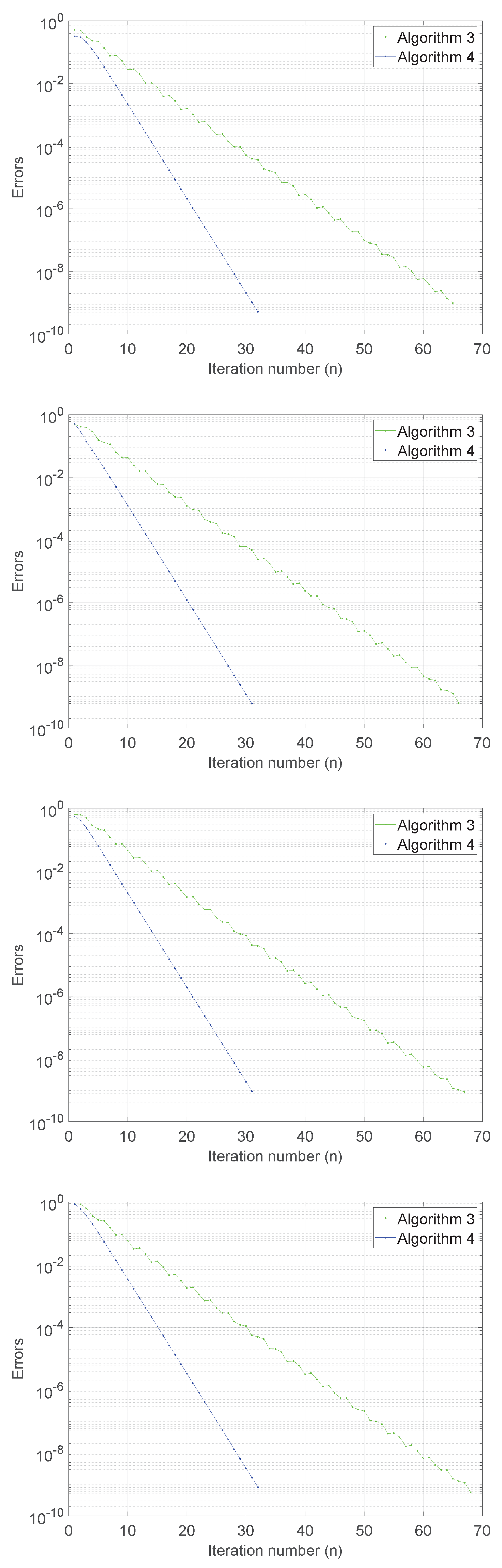
Now, we consider the mapping $S_i:{\mathbb{R}}^2\to {\mathbb{R}}^2$ defined by $S_{i}z={\left|\right|B\left|\right|}^{-1}Bz,$ for all $i,$ where $z={(x,y)}^T.$ It is easily verified that each $S_i$ is quasi-nonexpansive (note that in a Hilbert space relatively nonexpansive mapping reduces to quasi-nonexpansive mapping). The solution of the problem is $x^{†}={(0,0)}^T.$ We test the algorithms for three different starting points using $\left|\right|x_{n+1}-x_n\left|\right|<ϵ$ as stopping criterion, where $ϵ={10}^{-9}.$ The numerical result is reported in Figure 1 and

Table 1. Numerical results for Example 1.

		Algorithm 3	Algorithm 4
Case I	CPU Time (s)	0.0243	0.0241
	No of Iter.	65	32
Case II	CPU Time (s)	0.0120	0.0171
	No. of Iter.	66	31
Case III	CPU Time (s)	0.0117	0.0153
	No of Iter.	67	31
Case IV	CPU Time (s)	0.1770	0.1990
	No of Iter.	68	31

.

Case I: 

$x_1={(0,1)}^{\prime };$

Case II: 

$x_1={(1,0)}^{\prime };$

Case III: 

$x_1={(1,1)}^{\prime };$

Case IV: 

$x_1={(1,2)}^{\prime }.$

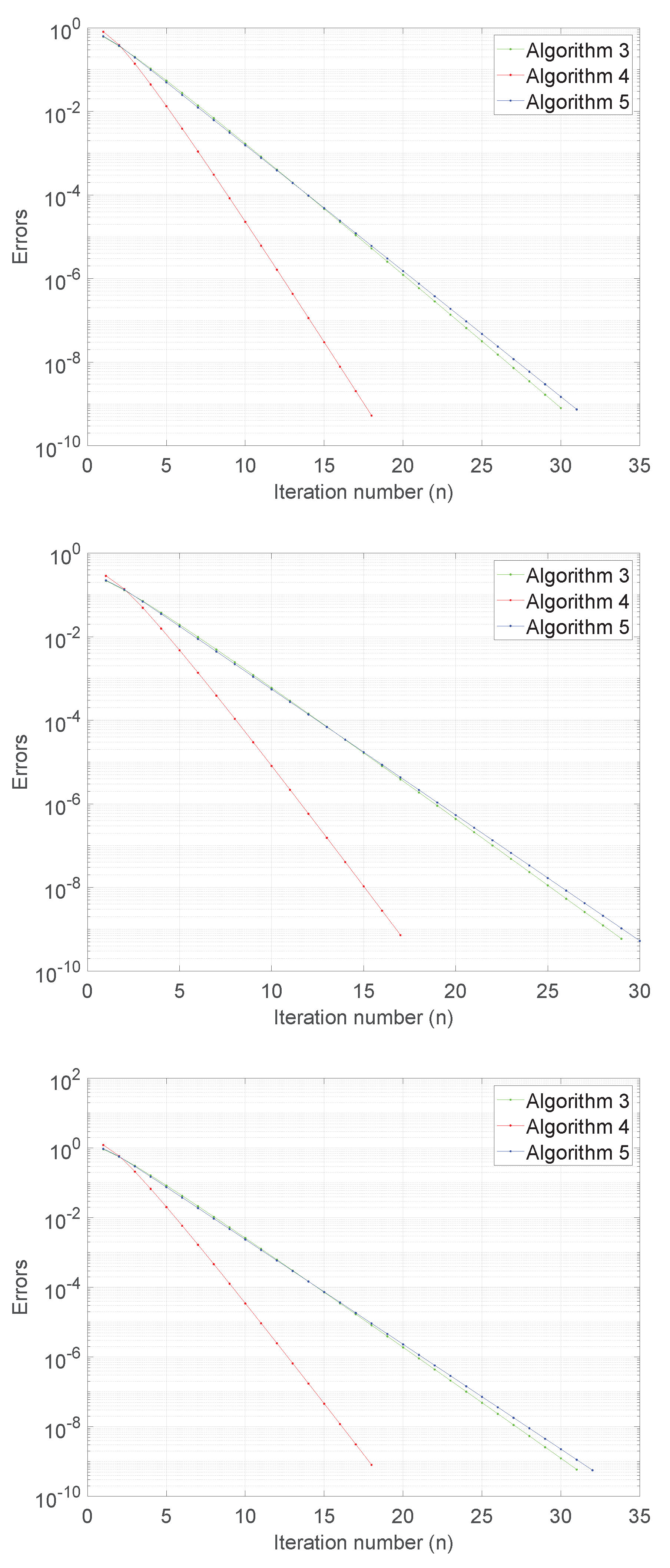
Example 2.

Suppose that $E=L^2\left([0,1]\right)$ with inner product

$$\langle x,y\rangle :={\int }_0^{1}x\left(t\right)y\left(t\right)dt,\forall x,y\in E,$$

and induced norm

$$\left|\right|x\left|\right|:=({\int }_0^1{\left|x\left(t\right)\right|}^2{dt)}^{\frac{1}{2}},\forall x\in E.$$

Let $C[0,1]$ denote the continuous function space defined on the interval $[0,1]$ and choose an arbitrary fixed $\phi \in C[0,1].$ Let $C:=\{x\in E:|\left|\phi x\right||\le 1\}.$ It can easily be verified that C is a nonempty closed convex subset of $E.$ Define an operator $A:E\to E^{*}$ by

$$\left(Ax\right)\left(t\right)=\max (0,x(t\left)\right),\forall x\in E.$$

Subsequently, A is two-Lipschitz continuous and monotone on E (see [64]). With these given C and $A,$ the solution set to the VIP (1) is given by $VI(C,A)=\left\{0\right\}\ne \varnothing .$ Define $g:E\to \mathbb{R}$ by

$$g\left(x\right)=\frac{1}{2}{\left(\right|\left|\phi x\right||}^2-1),\forall x\in E,$$

then g is a convex function and C is a level set of $g,$ i.e., $C=\{x\in E:g(x)\le 0\}.$ Also, g is differentiable on E and $\partial g\left(x\right)={\phi }^{2}x,\forall x\in E$ (see [65]). In this numerical example, we choose $\phi \left(t\right)=e^{-t},\forall t\in [0,1].$ Let $S_i:L^2\left([0,1]\right)\to L^2\left([0,1]\right)$ be defined by

$$\left(S_{i}x\right)\left(t\right)={\int }_0^1{t}^{i}x\left(s\right)ds,t\in [0,1].$$

Observe that $F\left(S_i\right)\ne \varnothing$ since $0\in F\left(S_i\right)$ for each $i\in \mathbb{N}.$ Moreover, $S_i$ are nonexpansive for each $i\in \mathbb{N},$ and, hence, quasi-nonexpansive. Therefore, the solution set of the problem is $x^{†}\left(t\right)=\left\{0\right\}.$ We test the algorithms for three different starting points using $\left|\right|x_n-x^{†}\left|\right|<ϵ$ as stopping criterion, where $ϵ={10}^{-9}.$ The numerical result is reported in Figure 2 and

Table 2. Numerical results for Example 2.

		Algorithm 3	Algorithm 4	Algorithm 5
Case I	CPU Time (s)	1.9220	1.9979	3.8269
	No of Iter.	30	18	31
Case II	CPU Time (s)	5.9673	8.1367	13.9678
	No. of Iter.	29	17	30
Case III	CPU Time (s)	2.4725	3.6332	5.8903
	No of Iter.	31	18	32

.

Case I: 

$x_1=t^3+3t^2-2;$

Case II: 

$x_1=\exp (-2t);$

Case III: 

$x_1=3\sin \left(2\pi t\right).$

6. Conclusions

In this paper, we studied a classical monotone and Lipschitz continuous variational inequality and fixed point problems defined on a level set of a convex function in the setting of Banach spaces. We proposed two iterative methods with self-adaptive step size that combine the Halpern method with a relaxed projection method for approximating a common solution of variational inequality and fixed point problems for an infinite family of relatively nonexpansive mappings in Banach spaces. The main advantage of our algorithms is to replace every projection onto the closed convex set with a projection onto some half-space which guarantees easy implementation of our proposed methods. Moreover, the step size can be adaptively selected. We obtained strong convergence results for the proposed methods without the knowledge of the Lipschitz constant of the monotone operator and we apply our results to finding a common solution of constrained convex minimization and fixed point problems in Banach spaces. The obtained results improve and extend several existing results in the current literature in this direction.

References

Fichera, G. Sul problema elastostatico di Signorini con ambigue condizioni al contorno. Atti Accad. Naz. Lincei VIII Ser. Rend. Cl. Sci. Fis. Mat. Nat.1963, 34, 138–142. [Google Scholar]
Stampacchia, G. Formes bilineaires coercitives sur les ensembles convexes. C. R. Acad. Sci. Paris1964, 258, 4413–4416. [Google Scholar]
Abass, H.A.; Aremu, K.O.; Jolaoso, L.O.; Mewomo, O.T. An inertial forward-backward splitting method for approximating solutions of certain optimization problems. J. Nonlinear Funct. Anal.2020. [Google Scholar] [CrossRef]
Gibali, A.; Reich, S.; Zalas, R. Outer approximation methods for solving variational inequalities in Hilbert space. Optimization2017, 66, 417–437. [Google Scholar] [CrossRef]
Jolaoso, L.O.; Alakoya, T.O.; Taiwo, A.; Mewomo, O.T. Inertial extragradient method via viscosity approximation approach for solving Equilibrium problem in Hilbert space. Optimization2020. [Google Scholar] [CrossRef]
Kassay, G.; Reich, S.; Sabach, S. Iterative methods for solving systems of variational inequalities in reflexive Banach spaces. SIAM J. Optim.2011, 21, 1319–1344. [Google Scholar] [CrossRef]
Mewomo, O.T.; Ogbuisi, F.U. Convergence analysis of an iterative method for solving multiple-set split feasibility problems in certain Banach spaces. Quaest. Math.2018, 41, 129–148. [Google Scholar] [CrossRef]
Jolaoso, L.O.; Alakoya, T.; Taiwo, A.; Mewomo, O.T. A parallel combination extragradient method with Armijo line searching for finding common solution of finite families of equilibrium and fixed point problems. Rend. del Circ. Mat. di Palermo Ser. 22019. [Google Scholar] [CrossRef]
Abbas, M.; Ibrahim, Y.; Khan, A.R.; De la Sen, M. Strong Convergence of a System of Generalized Mixed Equilibrium Problem, Split Variational Inclusion Problem and Fixed Point Problem in Banach Spaces. Symmetry2019, 11, 722. [Google Scholar] [CrossRef] [Green Version]
Alakoya, T.O.; Jolaoso, L.O.; Mewomo, O.T. A general iterative method for finding common fixed point of finite family of demicontractive mappings with accretive variational inequality problems in Banach spaces. Nonlinear Stud.2020, 27, 1–24. [Google Scholar]
Censor, Y.; Gibali, A.; Reich, S. Extensions of Korpelevich extragradient method for the variational inequality problem in Euclidean space. Optimization2012, 61, 1119–1132. [Google Scholar] [CrossRef]
Jolaoso, L.O.; Ogbuisi, F.U.; Mewomo, O.T. An iterative method for solving minimization, variational inequality and fixed point problems in reflexive Banach spaces. Adv. Pure Appl. Math.2017, 9, 167–184. [Google Scholar] [CrossRef]
Jolaoso, L.O.; Taiwo, A.; Alakoya, T.O.; Mewomo, O.T. A self adaptive inertial subgradient extragradient algorithm for variational inequality and common fixed point of multivalued mappings in Hilbert spaces. Demonstr. Math.2019, 52, 183–203. [Google Scholar] [CrossRef]
Jolaoso, L.O.; Taiwo, A.; Alakoya, T.O.; Mewomo, O.T. A unified algorithm for solving variational inequality and fixed point problems with application to the split equality problem. Comput. Appl. Math.2019. [Google Scholar] [CrossRef]
Jolaoso, L.O.; Taiwo, A.; Alakoya, T.O.; Mewomo, O.T. Strong convergence theorem for solving pseudo-monotone variational inequality problem using projection method in a reflexive Banach space. J. Optim. Theory Appl.2020. [Google Scholar] [CrossRef]
Kazmi, K.R.; Rizvi, S.H. An iterative method for split variational inclusion problem and fixed point problem for a nonexpansive mapping. Optim. Lett.2014, 8, 1113–1124. [Google Scholar] [CrossRef]
Ogwo, G.N.; Izuchukwu, C.; Aremu, K.O.; Mewomo, O.T. A viscosity iterative algorithm for a family of monotone inclusion problems in an Hadamard space. Bull. Belg. Math. Soc. Simon Stevin2020, 27, 125–152. [Google Scholar] [CrossRef]
Oyewole, O.K.; Abass, H.A.; Mewomo, O.T. A Strong convergence algorithm for a fixed point constrainted split null point problem. Rend. Circ. Mat. Palermo II2020. [Google Scholar] [CrossRef]
Taiwo, A.; Jolaoso, L.O.; Mewomo, O.T. General alternative regularization method for solving split equality common fixed point problem for quasi-pseudocontractive mappings in Hilbert spaces. Ric. Mat.2019. [Google Scholar] [CrossRef]
Taiwo, A.; Jolaoso, L.O.; Mewomo, O.T. Viscosity approximation method for solving the multiple-set split equality common fixed-point problems for quasi-pseudocontractive mappings in Hilbert Spaces. J. Ind. Manag. Optim.2020. [Google Scholar] [CrossRef]
Xu, Y. Ishikawa and Mann iterative processes with errors for nonlinear strongly accretive operator equations. J. Math. Anal. Appl.1998, 224, 91–101. [Google Scholar] [CrossRef] [Green Version]
Korpelevich, G.M. An extragradient method for finding saddle points and other problems. Ekon. Mat. Metody1976, 12, 747–756. [Google Scholar]
Ceng, L.C.; Hadjisavas, N.; Weng, N.C. Strong convergence theorems by a hybrid extragradient-like approximation method for variational inequalities and fixed point problems. J. Glob. Optim.2010, 46, 635–646. [Google Scholar] [CrossRef]
Censor, Y.; Gibali, A.; Reich, S. The subgradient extragradient method for solving variational inequalities in Hilbert space. J. Optim. Theory Appl.2011, 148, 318–335. [Google Scholar] [CrossRef] [PubMed] [Green Version]
Bauschke, H.H.; Combettes, P.L. A weak-to-strong convergence principle for Fejer-monotone methods in Hilbert spaces. Math. Oper. Res.2001, 26, 248–264. [Google Scholar] [CrossRef]
Okeke, G.A.; Abbas, M.; De La Sen, M. Approximation of the Fixed Point of Multivalued Quasi-Nonexpansive Mappings via a Faster Iterative Process with Applications. Discret. Dyn. Nat. Soc.2020. [Google Scholar] [CrossRef]
Wang, Y.; Fang, X.; Guan, J.L.; Kim, T.H. On split null point and common fixed point problems for multivalued demicontractive mappings. Optimization2020, 1–20. [Google Scholar] [CrossRef]
Aoyama, K.; Kimura, Y.; Takahashi, W.; Toyoda, M. Approximation of common fixed points of a countable family of nonexpansive mappings in a Banach space. Nonlinear Anal.2007, 67, 2350–2360. [Google Scholar] [CrossRef]
Shimoji, K.; Takahashi, W. Strong convergence to common fixed points of infinite nonexpansive mappings and applications. Taiwan J. Math.2001, 5, 387–404. [Google Scholar] [CrossRef]
Combettes, P.L. A block-iterative surrogate constraint splitting method for quadratic signal recovery. IEEE Trans. Signal Process.2003, 51, 1771–1782. [Google Scholar] [CrossRef] [Green Version]
Bauschke, H.H. The approximation of fixed points of compositions of nonexpansive mappings in Hilbert space. J. Math. Anal. Appl.1996, 202, 150–159. [Google Scholar] [CrossRef] [Green Version]
Youla, D.C. Mathematical theory of image restoration by the method of convex projections. In Image Recovery: Theory and Applications; Stark, H., Ed.; Academic Press: New York, NY, USA, 1987. [Google Scholar]
Iusem, A.N.; De Pierro, A.R. On the convergence of Han’s method for convex programming with quadratic objective. Math. Program. Ser. B1991, 52, 265–284. [Google Scholar] [CrossRef]
Iiduka, H. Acceleration method for convex optimization over the fixed point set of a nonexpansive mappings. Math. Prog. Ser. A2015, 149, 131–165. [Google Scholar] [CrossRef]
Iiduka, H. Fixed point optimization algorithm and its application to network bandwidth allocation. J. Comput. Appl. Math.2012, 236, 1733–1742. [Google Scholar] [CrossRef] [Green Version]
Luo, C.; Ji, H.; Li, Y. Utility-based multi-service bandwidth allocation in the 4G heterogeneous wireless networks. IEEE Wirel. Commun. Netw. Conf.2009. [Google Scholar] [CrossRef]
Maingé, P.E. A hybrid extragradient-viscosity method for monotone operators and fixed point problems. SIAM J. Control Optim.2008, 47, 1499–1515. [Google Scholar] [CrossRef]
Zhang, H.; Xu, Y.; Zhang, J. Reproducing Kernel Banach Spaces for Machine Learning. J. Mach. Learn. Res.2009, 10. [Google Scholar] [CrossRef] [Green Version]
Liu, Y. Strong convergence of the Halpern subgradient extragradient method for solving variational inequalities in Banach spaces. J. Nonlinear Sci. Appl.2017, 10, 395–409. [Google Scholar] [CrossRef]
Cioranescu, I. Geometry of Banach Spaces, Duality Mappings and Nonlinear Problems; Springer Science & Business Media: Berlin, Germany, 2012. [Google Scholar]
Taiwo, A.; Alakoya, T.O.; Mewomo, O.T. Halpern-type iterative process for solving split common fixed point and monotone variational inclusion problem between Banach spaces. Numer. Algorithms2020. [Google Scholar] [CrossRef]
Alber, Y.; Ryazantseva, I. Nonlinear Ill-Posed Problems of Monotone Type; Springer: London, UK, 2006. [Google Scholar]
Reich, S. A weak convergence theorem for the alternating method with Bregman distances. In Theory and Applications of Nonlinear Operators of Accretive and Monotone Type; Kartsatos, A.G., Ed.; Marcel Dekker: New York, NY, USA, 1996; pp. 313–318. [Google Scholar]
Kohsaka, F.; Takahashi, W. Existence and approximation of fixed points of firmly nonexpansive-type mappings in Banach spaces. SIAM J. Optim.2008, 19, 824–835. [Google Scholar] [CrossRef]
Hsu, M.H.; Takahashi, W.; Yao, J.C. Generalized hybrid mappings in Hilbert spaces and Banach spaces. Taiwan. J. Math.2012, 16, 129–149. [Google Scholar] [CrossRef]
Homaeipour, S.; Razani, A. Weak and strong convergence theorems for relatively nonexpansive multi-valued mappings in Banach spaces. Fixed Point Theory Appl.2011, 73. [Google Scholar] [CrossRef] [Green Version]
Kamimura, S.; Takahashi, W. Strong convergence of a proximal-type algorithm in a Banach space. SIAM J. Optim.2003, 13, 938–945. [Google Scholar] [CrossRef]
Xu, H.K. Strong convergence of approximating fixed point sequences for nonexpansive mappings. Bull. Aust. Math. Soc.2006, 74, 143–151. [Google Scholar] [CrossRef] [Green Version]
Iiduka, H.; Takahashi, W. Weak convergence of a projection algorithm for variational inequalities in a Banach space. J. Math. Anal. Appl.2008, 339, 668–679. [Google Scholar] [CrossRef]
Matsushita, S.Y.; Takahashi, W. A strong convergence theorem for relatively nonexpansive mappings in a Banach space. J. Approx. Theory2005, 134, 257–266. [Google Scholar] [CrossRef] [Green Version]
Nakajo, K. Strong convergence for gradient projection method and relatively nonexpansive mappings in Banach spaces. Appl. Math. Comput.2015, 271, 251–258. [Google Scholar] [CrossRef]
Chang, S.S.; Kim, J.K.; Wang, X.R. Modified block iterative algorithm for solving convex feasibility problems in Banach spaces. J. Inequal. Appl.2010, 869684. [Google Scholar] [CrossRef] [Green Version]
Alakoya, T.O.; Jolaoso, L.O.; Mewomo, O.T. Modified inertial subgradient extragradient method with self adaptive stepsize for solving monotone variational inequality and fixed point problems. Optimization2020. [Google Scholar] [CrossRef]
Ma, F. A subgradient extragradient algorithm for solving monotone variational inequalities in Banach spaces. J. Inequal. Appl.2020, 26. [Google Scholar] [CrossRef]
Aremu, K.O.; Abass, H.A.; Izuchukwu, C.; Mewomo, O.T. A viscosity-type algorithm for an infinitely countable family of (f,g)-generalized k-strictly pseudononspreading mappings in CAT(0) spaces. Analysis2020, 40, 19–37. [Google Scholar] [CrossRef]
Aremu, K.O.; Izuchukwu, C.; Ogwo, G.N.; Mewomo, O.T. Multi-step iterative algorithm for minimization and fixed point problems in p-uniformly convex metric spaces. J. Ind. Manag. Optim.2020. [Google Scholar] [CrossRef] [Green Version]
Ceng, L.C.; Ansari, Q.H.; Yao, J.C. Some iterative methods for finding fixed points and for solving constrained convex minimization problems. Nonlinear Anal.2011, 74, 5286–5302. [Google Scholar] [CrossRef]
Panyanak, B. Ishikawa iteration processes for multi-valued mappings in Banach Spaces. Comput. Math. Appl.2007, 54, 872–877. [Google Scholar] [CrossRef] [Green Version]
Tian, M.; Jiang, B. Inertial Haugazeau’s hybrid subgradient extragradient algorithm for variational inequality problems in Banach spaces. Optimization2020. [Google Scholar] [CrossRef]
Hieu, D.V.; Anh, P.K.; Muu, L.D. Modified hybrid projection methods for finding common solutions to variational inequality problems. Comput. Optim. Appl.2017, 66, 75–96. [Google Scholar] [CrossRef]
He, S.; Dong, Q.; Tian, H. Relaxed projection and contraction methods for solving Lipschitz continuous monotone variational inequalities. Rev. Real Acad. Cienc. Exatc. Fis. Nat. Ser. A Mat.2019, 113, 2773–2791. [Google Scholar] [CrossRef]
Figure 1.
Top: Case I; Next: Case II; Next: Case III; Bottom: Case IV.
Figure 2.
Top: Case I; Middle: Case II; Bottom: Case III.
Khan, S.H.; Alakoya, T.O.; Mewomo, O.T.