Using Statistical Modeling to Predict the Electrical Energy Consumption of an Electric Arc Furnace Producing Stainless Steel


Abstract
:1. Introduction
2. Background
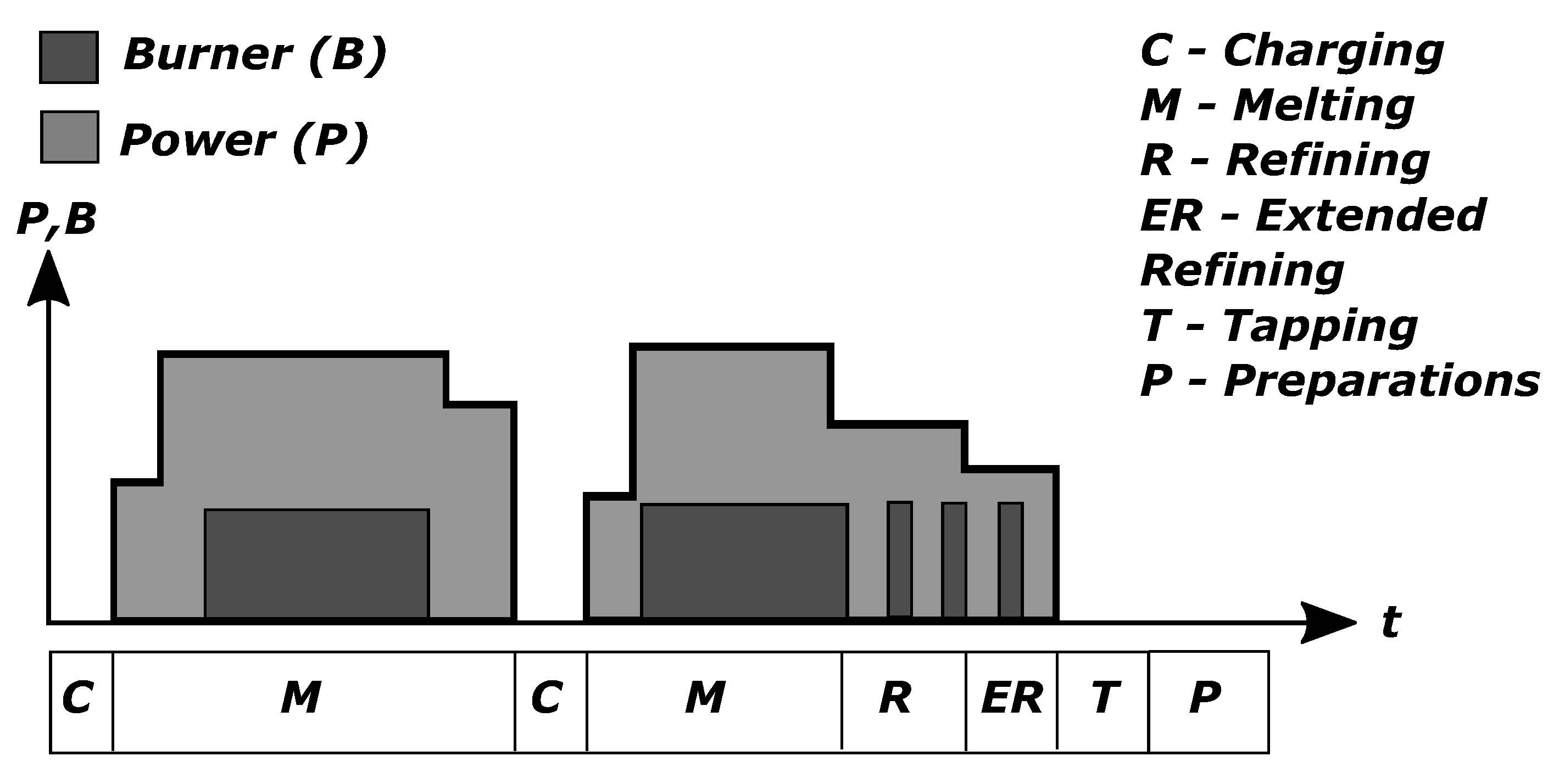
2.1. EAF Process
2.2. Energy Balance Equation
2.3. Non-Linearity
2.4. Statistical Modeling
- Select statistical model and values for the model-specific parameters.
- Train the model using training data until the model accuracy converges, i.e., stops improving.
- Test the model on previously unseen data.
- Record the accuracy on test data and evaluate its practical applicability.
- If the accuracy on the test data is satisfactory, deploy the model into production.
- Re-train the model if the model accuracy has deteriorated. This deterioration is bound to happen over time in a production setting, partly due to changes in the process.
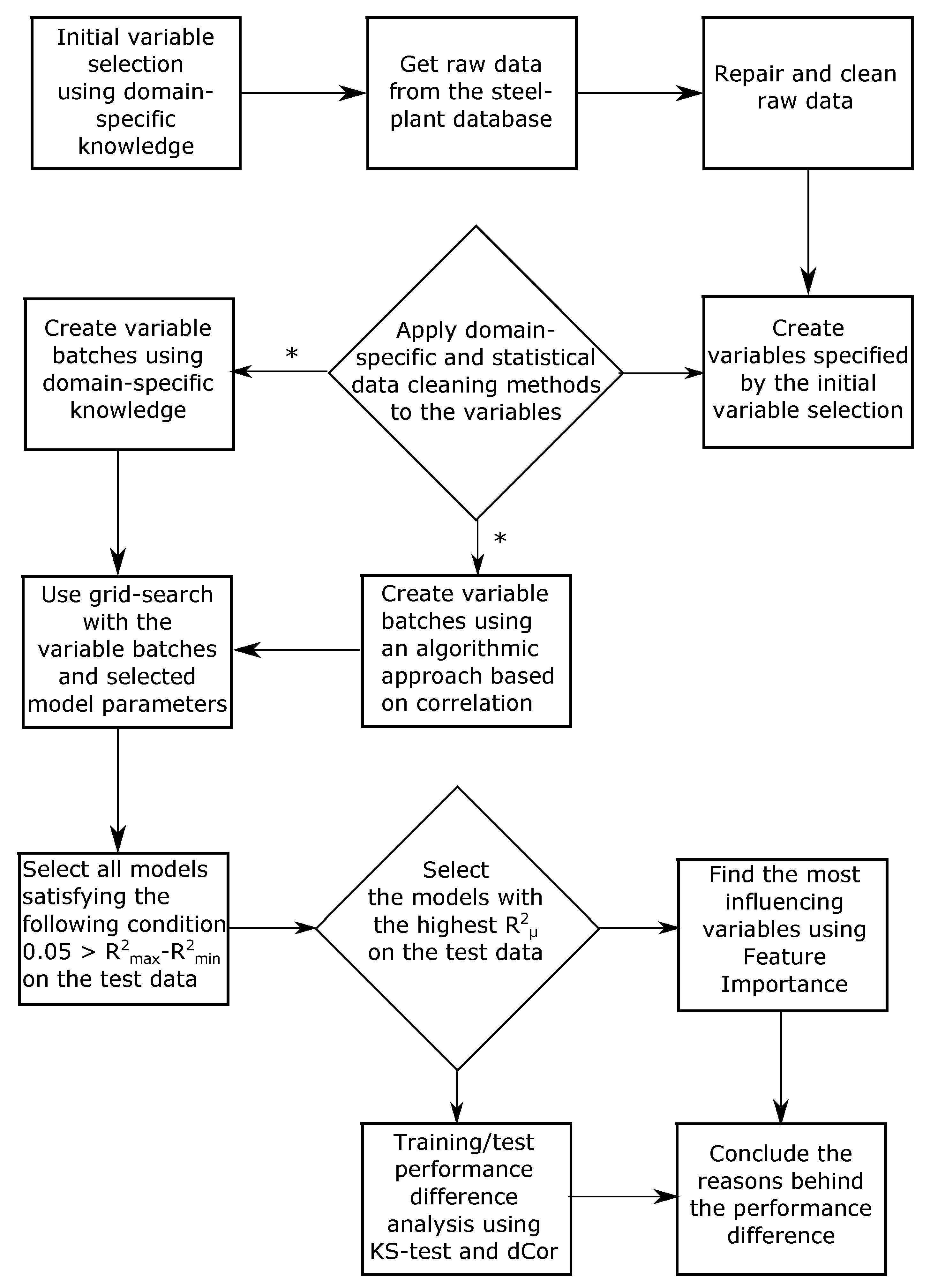
3. Method
3.1. Furnace Information
3.2. Data
3.2.1. Variable Selection
- Time: The logged times for the whole process as well as the various EAF sub-processes are important for predicting the EE demand. Each process sub-stage, Charging, Melting, Extended refining, Refining, and Tapping, contribute differently to the heat loss. For example, the heat loss is higher when molten steel is present compared to when the first bucket of scrap is charged. Both the TTT and the Process Time were included. The total time imposed by delays, defined as the sum of the deviation from nominal time of each EAF sub-process, was also included.Some obvious correlations can be expected with regards to these time variables. As Charging, Melting, Extended refining, Refining, and Tapping makes up the Process Time and the majority of TTT, these variables are expected to be relatively highly correlated.
- Chemical: Oxidation and the oxyfuel-burners can account for as much as 50% and 11% of the total ingoing energy, respectively (see Table 2). The contribution by the burners was accounted for by one variable propane. The oxygen gas injected through the burners was not included due to a near stoichiometric relationship between oxygen gas and propane (5:1). The wt.% of C, Si, Al, O of the total charged metallic material and the oxygen lancing were also included to account for exothermic chemical reactions occurring during the process.The wt.% Fe, Cr, and Ni of the total charged metallic material were included to account for possible deviations in the process due to the steel grade being produced.The contents of the charged oxide bearing raw material are, of course, expected to impact the thermodynamics and kinetics of each reaction. However, there are more complicated factors in play between the metallic elements in the steel melt and the oxides in the slag. To account for these complex effects, the following oxides, in wt.% of total charged oxide bearing raw material, were included: , , , , , and .It is known, by experience, that the specific heat per volume unit of oxygen is inversely proportional to total amount of lanced oxygen gas.
- Charged material: The different material types are expected to contribute differently to the melting behavior and heat transfer of the scrap. Hence, all 8 of the available Material Types were included in the list of input variables. The Total Weight of the ingoing material was included because it is closely connected to the required energy to melt the steel. It was also divided into two separate variables, Metal Weight and Slag Weight, which represent the total weight of metallic material and total weight of oxide bearing raw material, respectively.The sum of all Material Types equals the Total Weight. Hence, the Material Types are expected to be correlated with the Total Weight. Furthermore, the sum of the Slag Weight and Metal Weight equals the Total Weight and are also expected to be correlated.
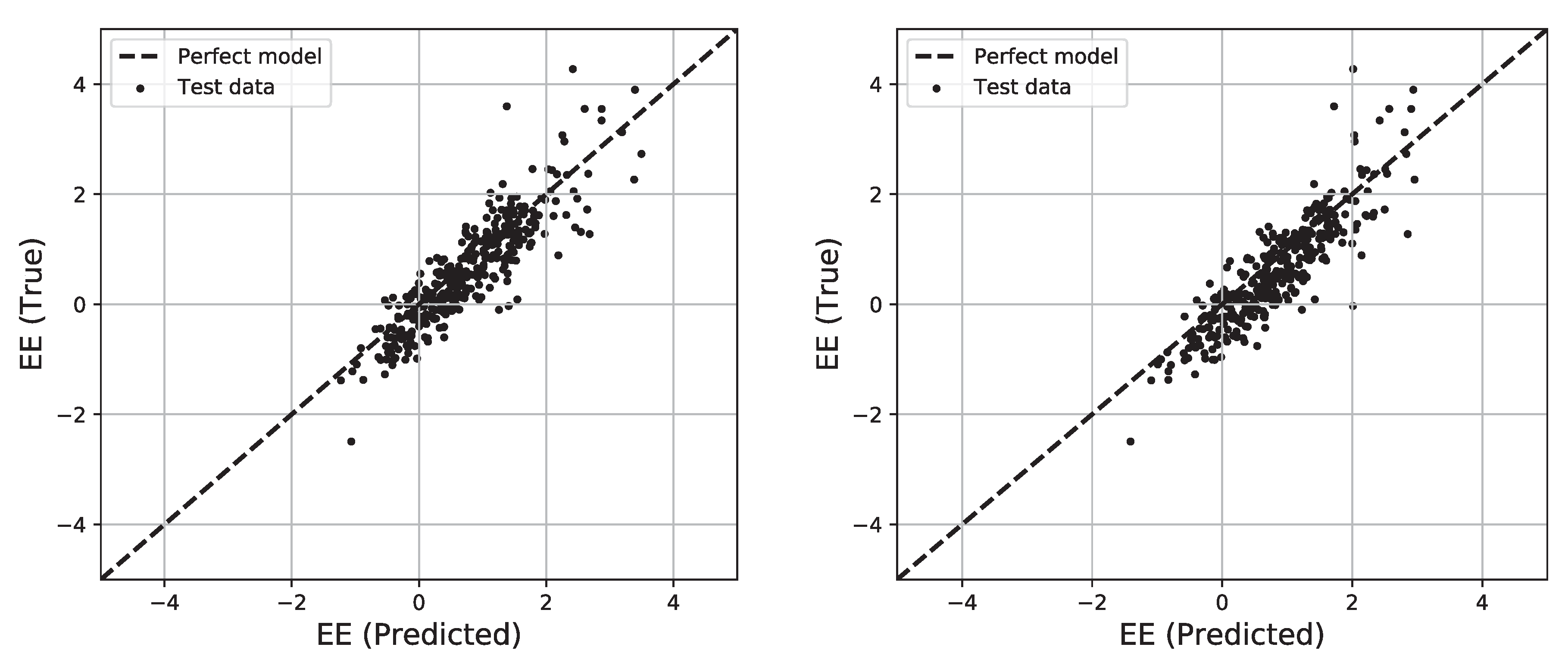
- Energy: There are numerous energy variables that can be included in the list of input variables. However, most are in one way or another connected to the already mentioned variables. For example, heat loss is linearly related to time and amount of ingoing scrap is linearly related to the heat required to heat and melt the scrap.The preheating energy was included because the actual preheating is conducted before the start of the EAF process itself. In the steel plant of study, the scrap is preheated with partial off-gas from the EAF operation. Hydrocarbons such as grease and oil, and moisture entrenched in the scrap are burned off. Due to the varying amounts of moisture and hydrocarbons in the scrap, the preheating energy as ingoing variable is therefore motivated.EE is well defined in the transformer system and is subject to a negligible error. This means that the logged EE value can be trusted and is therefore also taken as the true value when training the statistical model.
3.2.2. Variable Batches
3.2.3. Selection of Test Data
3.3. Data Treatment
3.3.1. Purpose
3.3.2. Domain-Specific Methods
3.3.3. Statistical Methods
- A more robust outlier detection algorithm was used in an attempt to remove outliers [47]. However, the resulting data set became too small after applying the algorithm on just a few of the variables.
- It makes sense to not apply statistical outlier detection methods on some variables. For example, the wt% content in the charged material can vary tremendously depending on what scrap types are available. Since multiple steel grades are produced using different charging strategies, the wt% of elements will also vary. Some stainless steel types need more wt% Cr and wt% Ni than others.
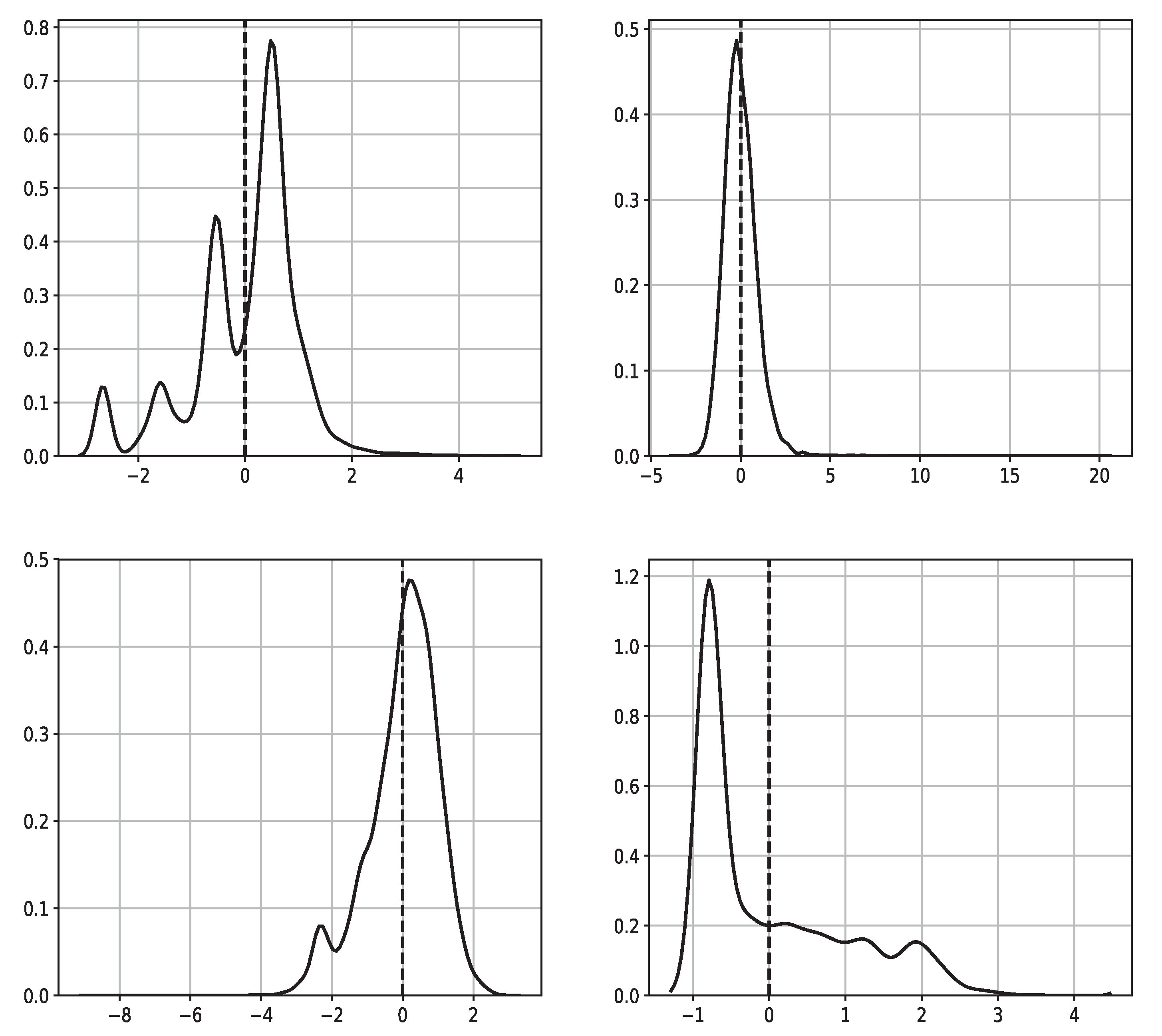
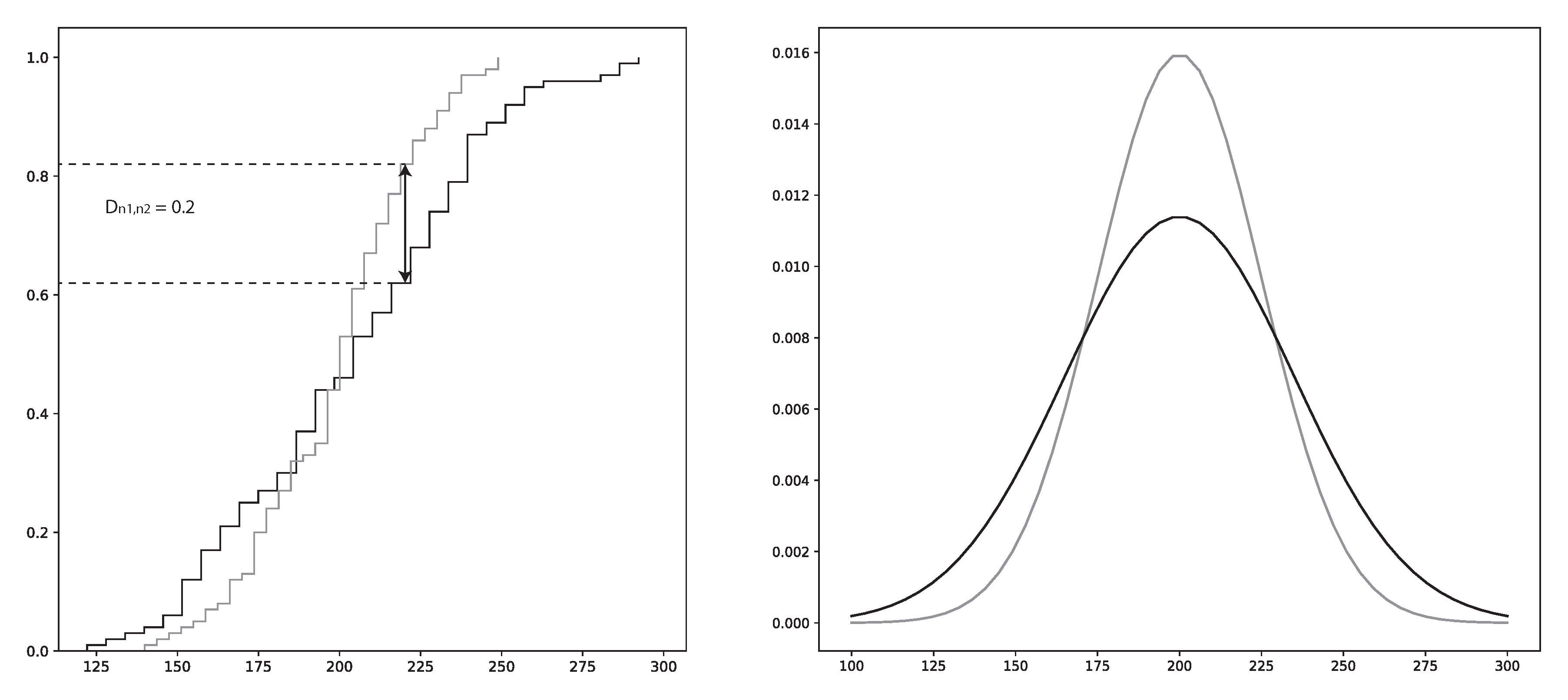
- Most conventional outlier detection methods assume that the data is normal distributed, or normal distributed with various levels of skewness and kurtosis. This is not always the case in EAF production data, see Figure 4.
3.4. Modeling
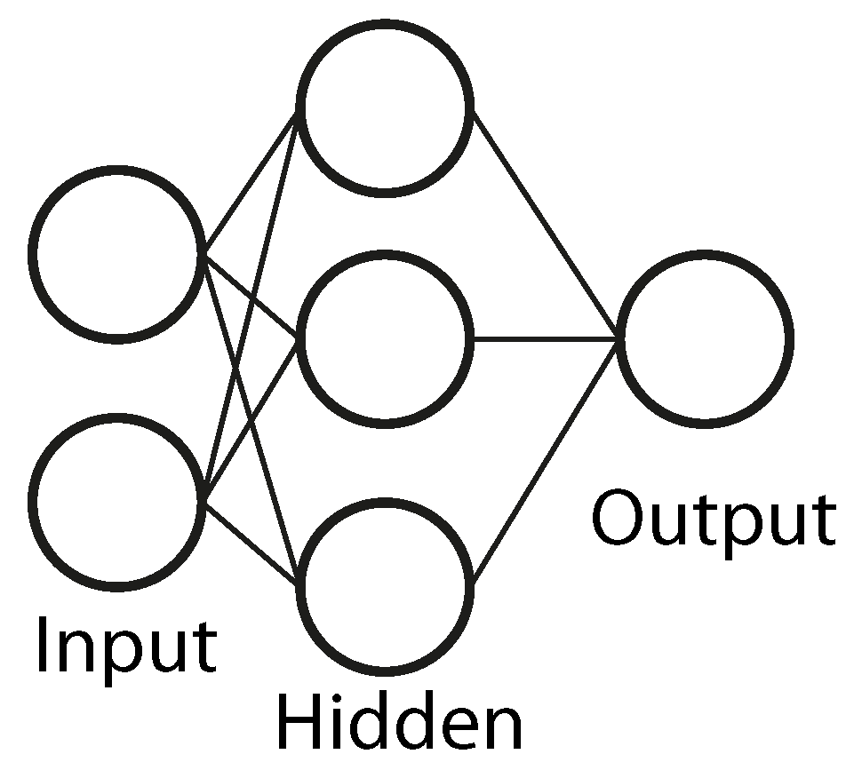
3.4.1. Artificial Neural Networks (ANN)
3.4.2. Model Performance Metrics
3.4.3. Hyperparameter Optimization
- Validation fraction: , which specifies the fraction of the training data used as validation set.
- Gradient-descent algorithm: An adaptive learning rate optimization algorithm known as Adam. This algorithm has been shown to outperform other gradient-descent algorithms in a variety of models and datasets. The algorithm-specific parameter values were selected as recommended in the paper [51].
- Early stopping set to True. Specified by the following items. 1. Number of iterations with no change = 20. Specifies how many iterations of increasing or equal performance are required before the training phase stops. 2. Tolerance = . The tolerance of improvement to reset the number of iterations with no change.
- Filter out any model that does not pass the following condition: . The motivation using this specific condition was to ensure that only stable models were selected while still enabling at least one model type from each variable batch to pass the condition.
- Sort the models on decreasing .
- Pick the first model in the list.
3.4.4. Algorithmic Approach
- Calculate the pair-wise correlation values between the input variables and the output variable (EE consumption).
- Use all input variables in the first model.
- For each subsequent model, remove the input variable with lowest correlation value with respect to the output variable. Save the performance metric results from all models for further analysis.
3.4.5. Model Analysis
- Train a model and record its error .
- Permute one of the input variables, , in the input matrix X.
- Apply the permuted input matrix, , to the trained model and record the error, .
- Repeat steps 2 and 3 for all input variables .
- Order all variables in the order of decreasing .
- Normalize all on (optional).
4. Results
4.1. Modeling
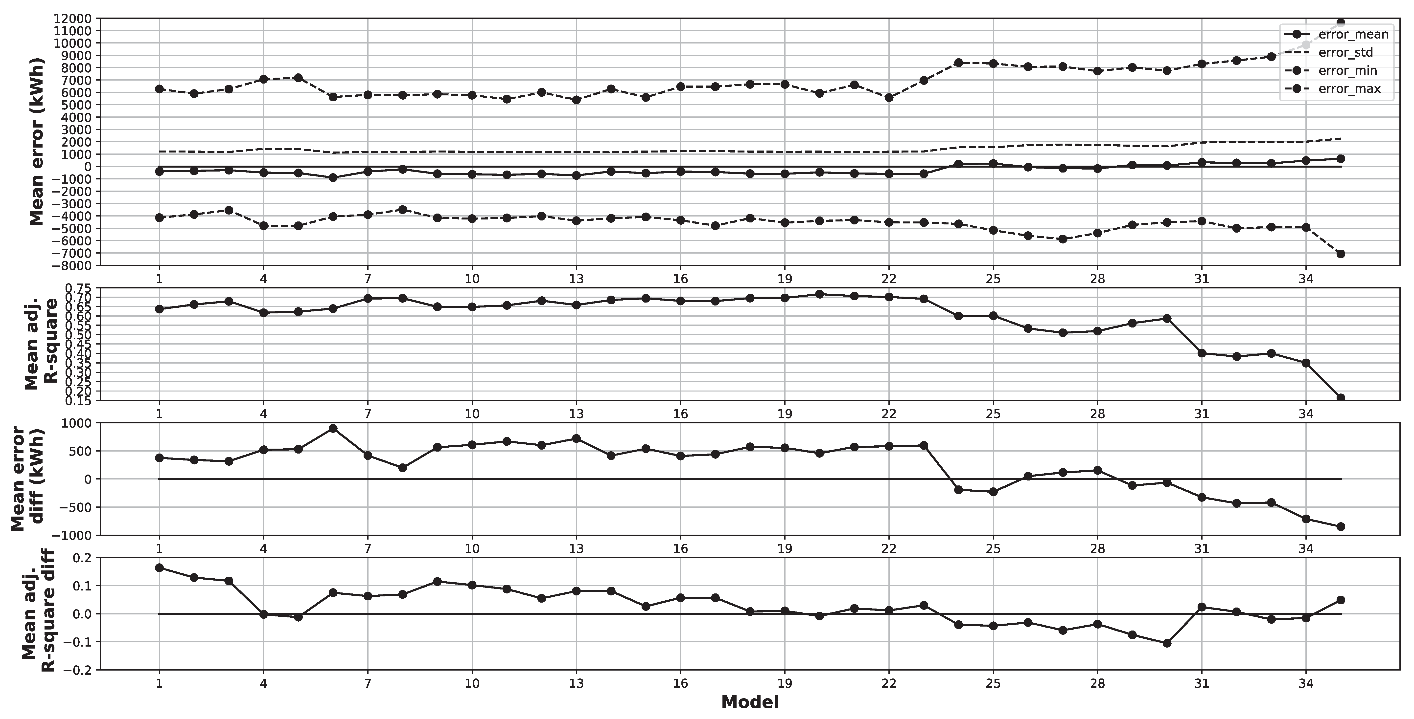
4.2. Model Analysis
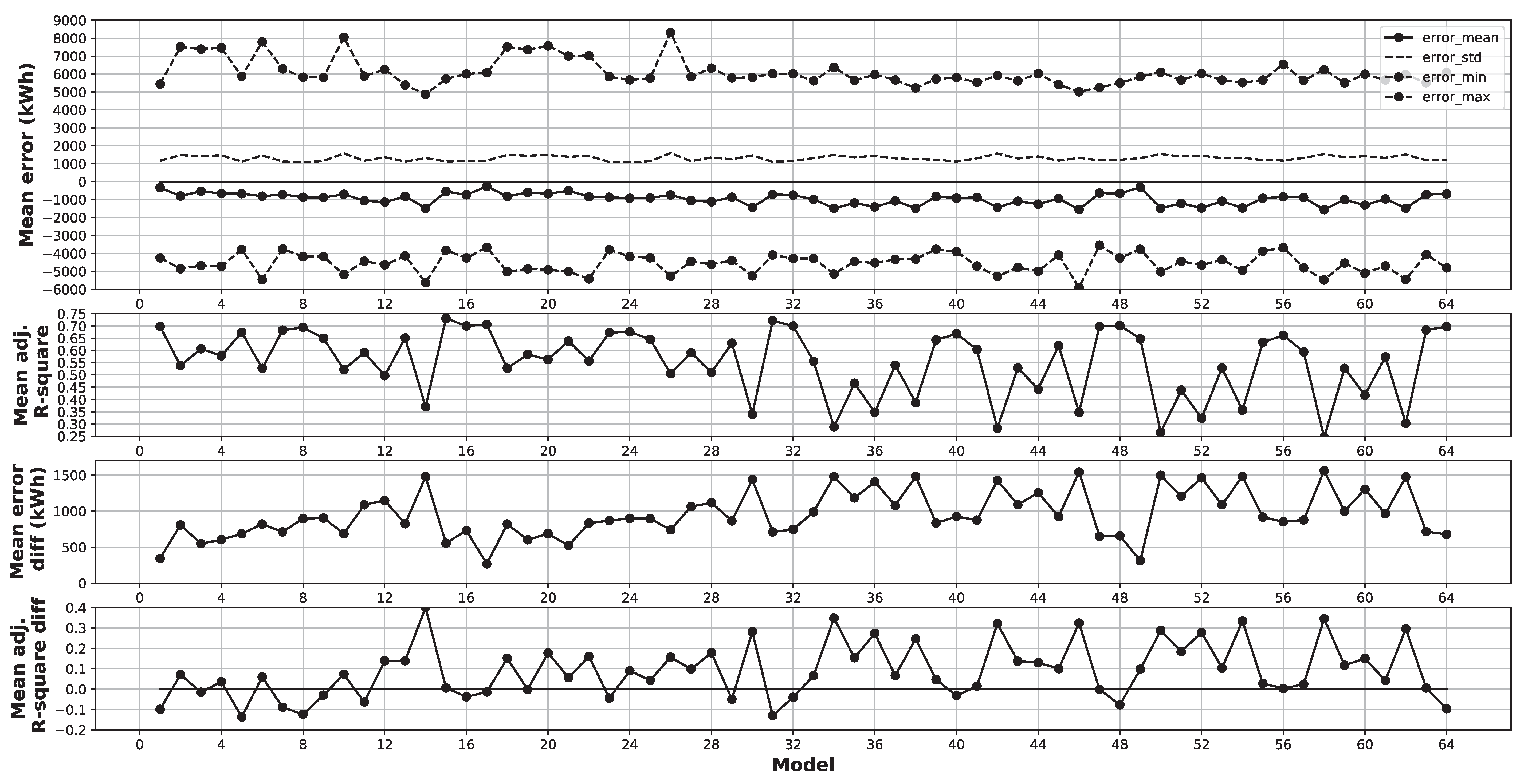
4.3. Grid-Search Metadata
5. Discussion
5.1. Modeling
5.2. Model Analysis
6. Conclusions
6.1. Modeling
- In the interest of model parsimony, increasing the number of input variables does not automatically increase model performance. This is both observed when comparing the best model from the experiments to the best model reported in the literature and when comparing model D64, which uses 6 variables, and model D1, which uses 35 variables. It is sufficient to choose several variables from an initial selection demarcated by the use of process knowledge.
- Similar performance was retrieved by the best models from the algorithmic approach and the domain approach, respectively. Given a setup of variables that are selected with process expertise, an algorithmic approach can find an optimal selection of variables. This is important from a practical applicability standpoint since less time need to be invested in searching for the optimal number of variables and the optimal subset of variables.
- Neural networks with many layers, increasing the model complexity, are not necessary to produce state-of-the-art model performance. This was observed both in the grid-search performed in the experiments and in comparing the best model from the experiments with the best models reported in the literature.
- The mean error is slightly higher, and the standard deviation of error is better for the best model compared to the best model reported in the literature. The minimum and maximum errors are approximately the same as the best model reported in the literature. However, these are −3.8 MWh to 5.7 MWh, respectively, which are quite high from a practical application context.
6.2. Model Analysis
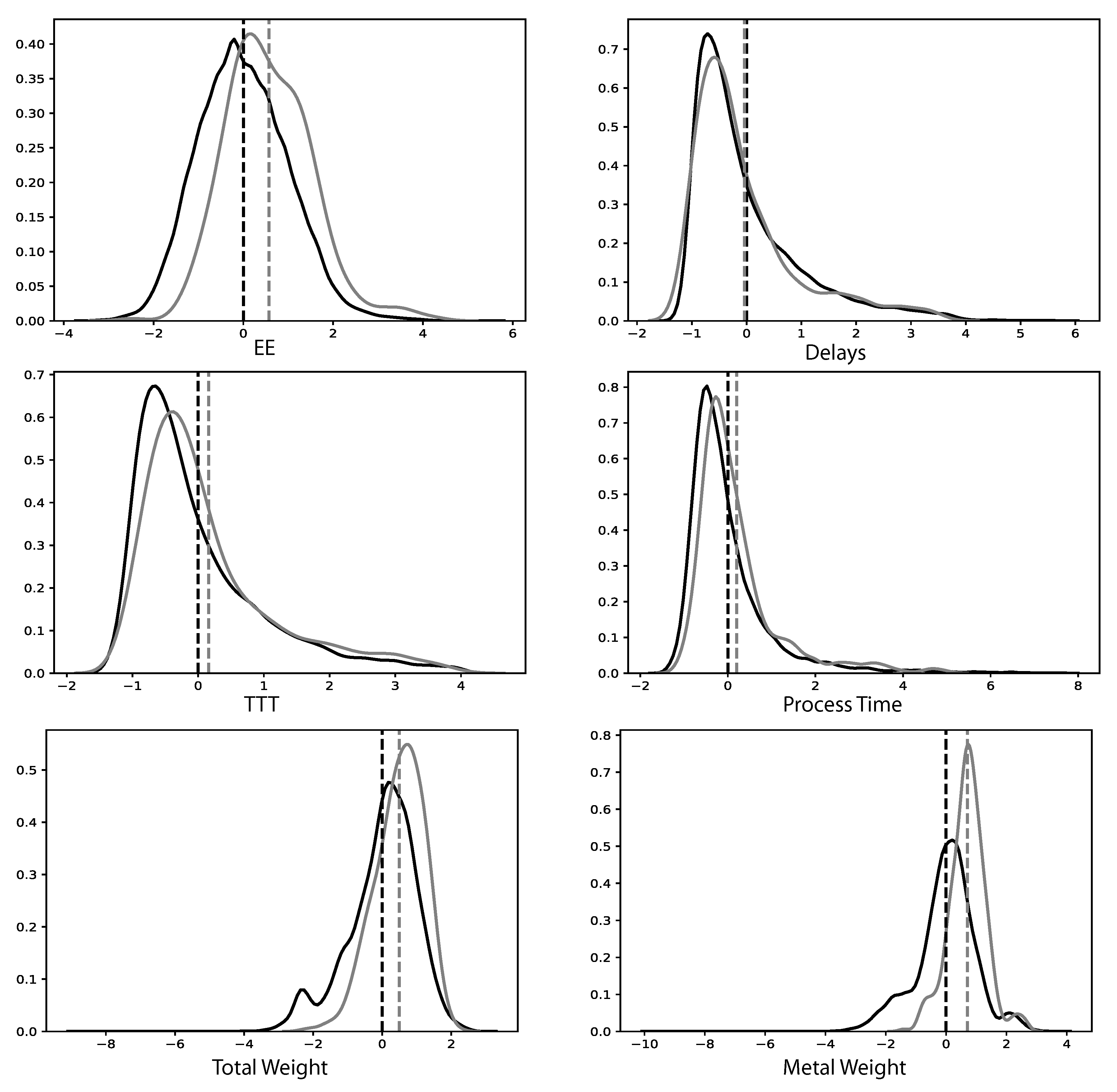
- Using KS test and FI as complementary tools, it was possible to identify an increase in Total Weight, Metal Weight, and Process Times as a highly probable cause behind the performance change from the training to test data for the 6 selected models.
- An analysis of the error from the selected models on the test data indicates that the models overestimate the EE consumption with regards to the change in the most important variables to the models. In particular, the Total Weight, Metal Weight, TTT, and Process Time variables.
- High intra-correlation between the metal composition, oxide composition, and raw material type variables was found using dCor on the training data. This explains why some of these variables get a high FI in some of the models. The changes in dCor from the training to test data were also prominent for these variables and can explain part of the performance changes for the selected models attributing higher FI to some of these metal composition, oxide composition, and raw material type variables.
6.3. Future Work
- Use upsampling on the training data to get more data points as outliers. Could potentially solve the problem with large maximum and minimum errors.
- Develop a more advanced variable selection algorithm based on dCor that takes into account one-to-many correlations for each input variable. The current algorithm only considers the correlation between the EE and each input variable.
- Apply dCor to groups of variables and the EE consumption instead of variables in a 1-to-1 fashion. This feature of dCor should be explored further.
- Use other non-linear correlation metrics to determine appropriate variable selection. These include Hoeffding’s, MI, and HHG.
- Investigate the effects of different types of scrap on the EE consumption using new classifications based on density, and heat and melting behavior.
- The effect on models by normalized variables that are not normally distributed is not known. See Figure 4 for a few examples.
Author Contributions
Funding
Acknowledgments
Conflicts of Interest
Nomenclature
| Total ingoing energy | |
| Total Electrical Energy (EE) output from transformer | |
| Total energy from chemical reactions in steel and slag | |
| Total energy input from burner | |
| Total outgoing energy | |
| Total energy output into steel | |
| Total energy lost in slag | |
| Total energy lost in gas | |
| Total energy lost in dust | |
| Total energy lost in cooling water | |
| Total energy lost through radiation | |
| Total energy lost through convection | |
| Total energy lost in electrical system and arc transfer | |
| The temperature of the cooling panels | |
| The temperature of the surface area subject to radiation losses | |
| Temperature of ingoing material and gas at the start of the EAF process | |
| Temperature of the steel at tapping | |
| Temperature of the off-gas leaving the EAF through the off-gas system | |
| Temperature of the cooling water | |
| The temperature of the surface area subject to convection losses | |
| The temperature of the air surrounding the EAF | |
| Mass of ingoing metallic material | |
| Mass of ingoing oxidic material | |
| Mass flow of dust in the off-gas system | |
| The heat capacity of steel at constant pressure | |
| The heat capacity of slag at constant pressure | |
| The heat capacity of dust at constant pressure | |
| The heat capacity of EAF ambient gas at constant pressure | |
| The heat capacity of reactants at constant pressure | |
| The heat capacity of products at constant pressure | |
| Standard heat of formation for reactants at 298K | |
| Standard heat of formation for products at 298K | |
| Heat of fusion for steel | |
| Heat of fusion for slag | |
| k | Conductivity of the cooling panels |
| h | Heat transfer coefficient of the EAF ambient gas |
| Emissivity factor of the radiating surface area of the EAF | |
| Stefan-Boltzmann constant | |
| Efficiency factor for the transformer system | |
| Efficiency factor for the energy transferred from the arcs | |
| Efficiency factor for burning the fuel in the burners | |
| Heat generated per volume unit of fuel | |
| Volume of the fuel consumed by the burners | |
| Surface area of the EAF subject to convection losses | |
| Surface area of the cooling panels | |
| Surface area of the EAF subject to radiation losses | |
| Average power of the transformer system | |
| P | Furnace pressure |
| M | Molar mass of the furnace gas |
| R | Universal gas constant |
| Volume flow of gas in the off-gas system | |
| Tap-to-tap time | |
| Power-on time | |
| Coefficient of determination | |
| Coefficient of determination adjusted for number of data points and variables | |
| n | Number of data points |
| p | Number of input variables |
| True value of the output variable for data point i | |
| Predicted value of the output variable for data point i | |
| P | Number of nodes in the previous layer. |
| Summation of the input values for jth node in the current layer. | |
| Weight of node i in the previous layer. | |
| Value of node i in the previous layer. | |
| Mean error of the mean error of the 10 model instances on the test data | |
| Standard deviation of the mean error of the 10 model instances on the test data | |
| Minimum of the mean error of the 10 model instances on the test data | |
| Maximum of the mean error of the 10 model instances on the test data | |
| Mean adjusted R-square of the 10 model instances | |
| Standard deviation of adjusted R-square of the 10 model instances | |
| Minimum of adjusted R-square of the 10 model instances | |
| Maximum of adjusted R-square of the 10 model instances | |
| Random variable | |
| Random variable | |
| Distance correlation between and | |
| Distance covariance between and | |
| Distance standard deviation for | |
| Distance standard deviation for | |
| Distance variance for | |
| Distance variance for | |
| Distance between values j and k for random variable | |
| Distance between values j and k for random variable | |
| Value j for random variable | |
| Value j for random variable | |
| Doubly centered distance for value j and k for random variable | |
| Doubly centered distance for value j and k for random variable | |
| Row mean of the distance matrix for the random variable | |
| Column mean of the distance matrix for the random variable | |
| Grand mean of the distance matrix for random variable | |
| Row mean of the distance matrix for the random variable | |
| Column mean of the distance matrix for the random variable | |
| Grand mean of the distance matrix for random variable | |
| Number of samples from the first distribution in the KS test | |
| Number of samples from the second distribution in the KS test | |
| KS-value from the KS test between and | |
| x | The total sample space in the KS test |
| First distribution function in the two-sample KS test | |
| Second distribution function in the two-sample KS test | |
| Null hypothesis | |
| Significance level | |
| c | Threshold value calculated from the cumulative KS distribution |
| L | Model error function |
| X | Input matrix |
| Input variable j | |
| Input matrix with permuted variable j | |
| Mean error | |
| Standard deviation of error |
Abbreviations
| CFD | Computational Fluid Dynamics |
| EE | Electrical Energy |
| EAF | Electric Arc Furnace |
| AC | Alternate Current |
| MLR | Multivariate Linear Regression |
| ANN | Artificial Neural Network |
| MSE | Mean Squared Error |
| FI | Feature Importance |
| KS | Kolmogorov–Smirnov |
| CDF | Cumulative distribution function |
| dCor | Distance correlation |
| MI | Mutual Information |
| HHG | Heller, Heller and Gorfine |
| TTT | Tap-to-Tap Time |
| TR | Training |
| TE | Test |
| NA | Not Available |
Appendix A
Appendix A.1. Hardware and Software

| Computer model | Dell Latitude E5570 |
| CPU | Intel Core i7 2376 MHz |
| RAM | 16,203 MB |
| Purpose | Software/Package | Version |
|---|---|---|
| Operating system | Microsoft Windows 7 Professional | 6.1.7601 Service Pack 1 Build 7601 |
| Programming language | Python 3 | 3.7.1 |
| Python distribution | Anaconda 3 | 4.6.7 |
| Data handling | Pandas | 0.23.4 |
| Numpy | 1.17.4 | |
| Statistical modeling | Scikit-learn | 0.20.1 |
| Feature importance | eli5 | 0.8.1 |
| Distance correlation | dcor | 0.3 |
| KS test | scipy | 0.15.0 |
| Visualization | Matplotlib | 3.0.2 |
Appendix A.2. Variable Batch Performance


Appendix A.3. Distance Correlation (dCor) Matrices
| Delays | TTT | Process | Charging | Ext. Ref. | Melting | Refining | Tapping | |
|---|---|---|---|---|---|---|---|---|
| Delays | 0.0 | −0.035 | −0.054 | 0.018 | −0.112 | −0.041 | −0.063 | −0.048 |
| TTT | −0.035 | 0.0 | −0.046 | 0.036 | −0.121 | −0.022 | −0.076 | −0.028 |
| Process | −0.054 | −0.046 | 0.0 | 0.074 | −0.212 | −0.009 | −0.059 | −0.009 |
| Charging | 0.018 | 0.036 | 0.074 | 0.0 | −0.058 | −0.088 | −0.078 | −0.059 |
| Ext. ref. | −0.112 | −0.121 | −0.212 | −0.058 | 0.0 | −0.103 | −0.015 | 0.007 |
| Melting | −0.041 | −0.022 | −0.009 | −0.088 | −0.103 | 0.0 | −0.017 | −0.067 |
| Ext. ref. | −0.063 | −0.076 | −0.059 | −0.078 | −0.015 | −0.017 | 0.0 | −0.002 |
| Tapping | −0.048 | −0.028 | −0.009 | −0.059 | 0.007 | −0.067 | −0.002 | 0.0 |
| Propane | −0.181 | −0.188 | −0.241 | −0.073 | −0.121 | −0.068 | −0.017 | −0.142 |
| O | −0.044 | −0.056 | −0.044 | −0.081 | −0.06 | −0.031 | −0.037 | −0.024 |
| TotWeight | −0.018 | 0.007 | 0.081 | −0.003 | −0.054 | −0.007 | −0.078 | 0.016 |
| Metal | −0.047 | −0.005 | 0.087 | −0.031 | −0.055 | −0.016 | −0.037 | 0.015 |
| Slag | −0.027 | −0.032 | −0.014 | −0.042 | −0.067 | −0.016 | 0.013 | −0.112 |
| %Fe | −0.043 | −0.034 | −0.052 | −0.008 | −0.125 | −0.056 | −0.092 | −0.028 |
| %O | −0.052 | −0.055 | −0.065 | −0.045 | −0.06 | −0.06 | −0.039 | −0.073 |
| %Al | −0.055 | −0.039 | −0.031 | −0.053 | −0.053 | −0.042 | −0.115 | −0.021 |
| %Cr | −0.056 | −0.06 | −0.021 | −0.036 | −0.068 | −0.056 | 0.022 | −0.049 |
| %Si | −0.048 | −0.055 | −0.077 | −0.058 | −0.058 | −0.052 | −0.113 | −0.093 |
| %C | −0.042 | −0.015 | −0.031 | −0.063 | −0.162 | −0.073 | 0.079 | −0.018 |
| %Ni | −0.067 | −0.059 | −0.09 | −0.028 | −0.112 | −0.06 | −0.078 | −0.039 |
| %FeO | −0.066 | −0.046 | −0.035 | −0.08 | −0.035 | −0.062 | −0.067 | −0.039 |
| %SiO | −0.044 | −0.041 | −0.031 | −0.041 | −0.068 | −0.057 | −0.116 | −0.058 |
| %AlO | −0.089 | −0.076 | −0.056 | −0.134 | −0.088 | −0.043 | −0.166 | −0.041 |
| %CrO | −0.116 | −0.128 | −0.072 | −0.112 | −0.114 | −0.05 | −0.119 | −0.031 |
| %Mgo | −0.074 | −0.082 | −0.087 | −0.044 | −0.056 | −0.026 | −0.038 | −0.021 |
| %CaO | −0.039 | −0.029 | −0.026 | −0.048 | −0.065 | −0.045 | −0.084 | −0.054 |
| Type A | −0.061 | −0.062 | −0.054 | −0.051 | −0.059 | −0.073 | −0.229 | −0.041 |
| Type B | −0.033 | −0.03 | −0.055 | −0.053 | −0.088 | −0.038 | −0.016 | −0.057 |
| Type C | −0.006 | −0.016 | −0.049 | −0.012 | −0.035 | −0.078 | −0.192 | −0.054 |
| Type D | −0.036 | −0.026 | −0.038 | −0.033 | −0.063 | −0.077 | −0.137 | −0.03 |
| Type E | −0.049 | −0.054 | −0.056 | −0.047 | −0.058 | −0.062 | −0.015 | −0.088 |
| Type F | −0.034 | −0.022 | −0.023 | −0.043 | −0.02 | −0.042 | −0.071 | −0.096 |
| Type G | −0.06 | −0.07 | −0.161 | −0.038 | −0.112 | −0.081 | −0.202 | −0.076 |
| Type N | −0.133 | −0.164 | −0.127 | −0.048 | −0.126 | −0.087 | −0.091 | −0.031 |
| PreHeater | −0.055 | −0.055 | −0.029 | −0.069 | −0.066 | −0.052 | −0.151 | −0.066 |
| EE | −0.135 | −0.134 | −0.135 | −0.07 | −0.226 | 0.02 | −0.051 | 0.023 |
| Propane | O2 | TotWeight | Metal | Slag | %Fe | %O | %Al | |
| Delays | −0.181 | −0.044 | −0.018 | −0.047 | −0.027 | −0.043 | −0.052 | −0.055 |
| TTT | −0.188 | −0.056 | 0.007 | −0.005 | −0.032 | −0.034 | −0.055 | −0.039 |
| Process | −0.241 | −0.044 | 0.081 | 0.087 | −0.014 | −0.052 | −0.065 | −0.031 |
| Charging | −0.073 | −0.081 | −0.003 | −0.031 | −0.042 | −0.008 | −0.045 | −0.053 |
| Remelting | −0.121 | −0.06 | −0.054 | −0.055 | −0.067 | −0.125 | −0.06 | −0.053 |
| Melting | −0.068 | −0.031 | −0.007 | −0.016 | −0.016 | −0.056 | −0.06 | −0.042 |
| Ext. ref. | −0.017 | −0.037 | −0.078 | −0.037 | 0.013 | −0.092 | −0.039 | −0.115 |
| Tapping | −0.142 | −0.024 | 0.016 | 0.015 | −0.112 | −0.028 | −0.073 | −0.021 |
| Propane | 0.0 | 0.174 | 0.201 | 0.197 | −0.057 | −0.077 | −0.144 | 0.012 |
| O | 0.174 | 0.0 | 0.135 | 0.141 | −0.025 | −0.048 | −0.049 | −0.022 |
| TotWeight | 0.201 | 0.135 | 0.0 | 0.001 | −0.219 | −0.08 | −0.209 | 0.076 |
| Metal | 0.197 | 0.141 | 0.001 | 0.0 | −0.058 | −0.186 | −0.154 | −0.096 |
| Slag | −0.057 | −0.025 | −0.219 | −0.058 | 0.0 | 0.098 | −0.066 | 0.155 |
| %Fe | −0.077 | −0.048 | −0.08 | −0.186 | 0.098 | 0.0 | −0.075 | 0.025 |
| %O | −0.144 | −0.049 | −0.209 | −0.154 | −0.066 | −0.075 | 0.0 | −0.089 |
| %Al | 0.012 | −0.022 | 0.076 | −0.096 | 0.155 | 0.025 | −0.089 | 0.0 |
| %Cr | −0.038 | −0.02 | 0.044 | −0.125 | 0.018 | 0.133 | −0.038 | −0.066 |
| %Si | −0.025 | 0.045 | −0.219 | −0.041 | −0.094 | −0.183 | −0.326 | −0.059 |
| %C | 0.056 | −0.126 | −0.012 | −0.034 | −0.046 | −0.007 | −0.068 | −0.004 |
| %Ni | −0.058 | −0.055 | −0.137 | −0.254 | 0.118 | −0.058 | −0.081 | 0.033 |
| %FeO | 0.062 | 0.049 | 0.09 | −0.066 | 0.141 | −0.055 | −0.139 | −0.05 |
| %SiO | 0.017 | −0.003 | 0.143 | −0.131 | 0.222 | −0.122 | −0.145 | −0.046 |
| %AlO | −0.168 | −0.059 | −0.011 | −0.125 | −0.054 | −0.125 | −0.296 | −0.133 |
| %CrO | −0.127 | −0.098 | 0.056 | −0.194 | 0.193 | −0.182 | −0.088 | −0.108 |
| %MgO | −0.035 | 0.065 | −0.018 | −0.079 | 0.117 | −0.180 | −0.236 | 0.030 |
| %CaO | 0.038 | 0.014 | 0.123 | −0.145 | 0.264 | −0.119 | −0.223 | −0.052 |
| Type A | −0.036 | −0.042 | −0.211 | −0.292 | −0.025 | −0.171 | −0.093 | −0.224 |
| Type B | −0.057 | −0.047 | −0.089 | −0.099 | −0.036 | −0.168 | −0.214 | −0.095 |
| Type C | −0.02 | 0.003 | −0.110 | −0.119 | −0.085 | −0.054 | −0.15 | −0.071 |
| Type D | −0.047 | −0.019 | −0.140 | −0.144 | 0.01 | 0.0 | −0.094 | −0.109 |
| Type E | −0.123 | −0.02 | −0.160 | −0.130 | 0.043 | −0.117 | −0.189 | −0.027 |
| Type F | −0.025 | 0.018 | −0.02 | −0.036 | −0.034 | −0.096 | −0.114 | −0.038 |
| Type G | −0.028 | 0.150 | −0.205 | 0.006 | 0.101 | −0.366 | −0.344 | −0.241 |
| Type N | 0.164 | 0.244 | 0.106 | 0.135 | −0.089 | −0.108 | −0.104 | −0.036 |
| PreHeater | −0.055 | −0.035 | −0.066 | −0.043 | −0.137 | −0.095 | −0.06 | −0.086 |
| EE | −0.135 | 0.009 | 0.209 | 0.208 | −0.071 | −0.086 | −0.225 | −0.042 |
| %Cr | %Si | %C | %Ni | %FeO | %SiO2 | %Al2O3 | ||
| Delays | −0.056 | −0.048 | −0.042 | −0.067 | −0.066 | −0.044 | −0.089 | |
| TTT | −0.06 | −0.055 | −0.015 | −0.059 | −0.046 | −0.041 | −0.076 | |
| Process | −0.021 | −0.077 | −0.031 | −0.09 | −0.035 | −0.031 | −0.056 | |
| Charging | −0.036 | −0.058 | −0.063 | −0.028 | −0.08 | −0.041 | −0.134 | |
| Ext. ref. | −0.068 | −0.058 | −0.162 | −0.112 | −0.035 | −0.068 | −0.088 | |
| Melting | −0.056 | −0.052 | −0.073 | −0.06 | −0.062 | −0.057 | −0.043 | |
| Refining | 0.022 | −0.113 | 0.079 | −0.078 | −0.067 | −0.116 | −0.166 | |
| TT | −0.049 | −0.093 | −0.018 | −0.039 | −0.039 | −0.058 | −0.041 | |
| Propane | −0.038 | −0.025 | 0.056 | −0.058 | 0.062 | 0.017 | −0.168 | |
| O | −0.02 | 0.045 | −0.126 | −0.055 | 0.049 | −0.003 | −0.059 | |
| TotWeight | 0.044 | −0.219 | −0.012 | −0.137 | 0.09 | 0.143 | −0.011 | |
| Metal | −0.125 | −0.041 | −0.034 | −0.254 | −0.066 | −0.131 | −0.125 | |
| Slag | 0.018 | −0.094 | −0.046 | 0.118 | 0.141 | 0.222 | −0.054 | |
| %Fe | 0.133 | −0.183 | −0.007 | −0.058 | −0.055 | −0.122 | −0.125 | |
| %O | −0.038 | −0.326 | −0.068 | −0.081 | −0.139 | −0.145 | −0.296 | |
| %Al | −0.066 | −0.059 | −0.004 | 0.033 | −0.05 | −0.046 | −0.133 | |
| %Cr | 0.0 | −0.066 | 0.028 | 0.016 | −0.136 | −0.092 | −0.135 | |
| %Si | −0.066 | 0.0 | −0.146 | −0.184 | −0.101 | −0.225 | −0.337 | |
| %C | 0.028 | −0.146 | 0.0 | −0.04 | 0.024 | 0.035 | −0.069 | |
| %Ni | 0.016 | −0.184 | −0.04 | 0.0 | −0.047 | −0.065 | −0.130 | |
| %FeO | −0.136 | −0.101 | 0.024 | −0.047 | 0.0 | −0.04 | 0.025 | |
| %SiO | −0.092 | −0.225 | 0.035 | −0.065 | −0.04 | 0.0 | −0.082 | |
| %AlO | −0.135 | −0.337 | −0.069 | −0.130 | 0.025 | −0.082 | 0.0 | |
| %CrO | −0.009 | −0.258 | −0.006 | −0.118 | −0.087 | −0.091 | 0.116 | |
| %MgO | −0.058 | −0.196 | 0.025 | −0.158 | 0.053 | −0.016 | −0.351 | |
| %CaO | −0.077 | −0.238 | 0.045 | −0.053 | −0.110 | −0.071 | −0.117 | |
| Type A | −0.143 | −0.174 | −0.065 | −0.185 | −0.244 | −0.049 | 0.129 | |
| Type B | −0.084 | −0.213 | −0.053 | −0.106 | −0.089 | −0.165 | −0.177 | |
| Type C | 0.003 | −0.155 | 0.085 | −0.058 | 0.027 | −0.06 | −0.261 | |
| Type D | −0.004 | −0.131 | 0.183 | −0.017 | −0.05 | −0.039 | −0.194 | |
| Type E | −0.015 | −0.217 | −0.029 | −0.087 | −0.165 | −0.197 | −0.238 | |
| Type F | −0.021 | −0.165 | −0.041 | −0.065 | −0.018 | −0.056 | −0.036 | |
| Type G | −0.212 | −0.231 | −0.154 | −0.291 | −0.112 | −0.339 | −0.122 | |
| Type N | −0.043 | 0.068 | 0.021 | −0.126 | −0.028 | −0.056 | −0.094 | |
| PreHeater | −0.092 | −0.04 | −0.112 | −0.096 | 0.043 | −0.036 | −0.119 | |
| EE | −0.008 | −0.111 | 0.129 | −0.09 | −0.091 | −0.032 | −0.08 | |
| %Cr2O3 | %MgO | %CaO | Type A | Type B | Type C | Type D | Type E | |
| Delays | −0.116 | −0.074 | −0.039 | −0.061 | −0.033 | −0.006 | −0.036 | −0.049 |
| TTT | −0.128 | −0.082 | −0.029 | −0.062 | −0.03 | −0.016 | −0.026 | −0.054 |
| Process | −0.072 | −0.087 | −0.026 | −0.054 | −0.055 | −0.049 | −0.038 | −0.056 |
| Charging | −0.112 | −0.044 | −0.048 | −0.051 | −0.053 | −0.012 | −0.033 | −0.047 |
| Ext. ref. | −0.114 | −0.056 | −0.065 | −0.059 | −0.088 | −0.035 | −0.063 | −0.058 |
| Melting | −0.05 | −0.026 | −0.045 | −0.073 | −0.038 | −0.078 | −0.077 | −0.062 |
| Refining | −0.119 | −0.038 | −0.084 | −0.229 | −0.016 | −0.192 | −0.137 | −0.015 |
| Tapping | −0.031 | −0.021 | −0.054 | −0.041 | −0.057 | −0.054 | −0.03 | −0.088 |
| Propane | −0.127 | −0.035 | 0.038 | −0.036 | −0.057 | −0.02 | −0.047 | −0.123 |
| O | −0.098 | 0.065 | 0.014 | −0.042 | −0.047 | 0.003 | −0.019 | −0.02 |
| TotWeight | 0.056 | −0.018 | 0.123 | −0.211 | −0.089 | −0.110 | −0.140 | −0.160 |
| Metal | −0.194 | −0.079 | −0.145 | −0.292 | −0.099 | −0.119 | −0.144 | −0.130 |
| Slag | 0.193 | 0.117 | 0.264 | −0.025 | −0.036 | −0.085 | 0.01 | 0.043 |
| %Fe | −0.182 | −0.180 | −0.119 | −0.171 | −0.168 | −0.054 | 0.0 | −0.117 |
| %O | −0.088 | −0.236 | −0.223 | −0.093 | −0.214 | −0.150 | −0.094 | −0.189 |
| %Al | −0.108 | 0.03 | −0.052 | −0.224 | −0.095 | −0.071 | −0.109 | −0.027 |
| %Cr | −0.009 | −0.058 | −0.077 | −0.143 | −0.084 | 0.003 | −0.004 | −0.015 |
| %Si | −0.258 | −0.196 | −0.238 | −0.174 | −0.213 | −0.155 | −0.131 | −0.217 |
| %C | −0.006 | 0.025 | 0.045 | −0.065 | −0.053 | 0.085 | 0.183 | −0.029 |
| %Ni | −0.118 | −0.158 | −0.053 | −0.185 | −0.106 | −0.058 | −0.017 | −0.087 |
| %FeO | −0.087 | 0.053 | −0.110 | −0.244 | −0.089 | 0.027 | −0.05 | −0.165 |
| %SiO | −0.091 | −0.016 | −0.071 | −0.049 | −0.165 | −0.06 | −0.039 | −0.197 |
| %AlO | 0.116 | −0.351 | −0.117 | 0.129 | −0.177 | −0.261 | −0.194 | −0.238 |
| %CrO | 0.0 | −0.226 | −0.052 | 0.03 | −0.141 | −0.136 | −0.017 | −0.173 |
| %Mgo | −0.226 | 0.0 | −0.254 | −0.126 | −0.206 | −0.033 | −0.044 | −0.164 |
| %CaO | −0.052 | −0.254 | 0.0 | −0.076 | −0.236 | −0.003 | −0.008 | −0.243 |
| Type A | 0.03 | −0.126 | −0.076 | 0.0 | −0.106 | −0.225 | −0.226 | −0.127 |
| Type B | −0.141 | −0.206 | −0.236 | −0.106 | 0.0 | 0.011 | −0.025 | −0.210 |
| Type C | −0.136 | −0.033 | −0.003 | −0.225 | 0.011 | 0.0 | −0.122 | −0.065 |
| Type D | −0.017 | −0.044 | −0.008 | −0.226 | −0.025 | −0.122 | 0.0 | −0.01 |
| Type E | −0.173 | −0.164 | −0.243 | −0.127 | −0.210 | −0.065 | −0.01 | 0.0 |
| Type F | 0.017 | −0.034 | −0.058 | −0.065 | −0.028 | 0.006 | −0.084 | −0.118 |
| Type G | −0.398 | −0.048 | −0.302 | −0.256 | −0.072 | −0.209 | −0.281 | −0.230 |
| Type N | −0.088 | −0.086 | −0.054 | −0.107 | −0.054 | −0.039 | −0.063 | −0.078 |
| PreHeater | −0.179 | 0.027 | −0.05 | −0.112 | −0.062 | −0.091 | −0.124 | −0.015 |
| EE | −0.004 | −0.048 | −0.074 | −0.03 | −0.069 | −0.141 | −0.084 | −0.172 |
| Type F | Type G | Type N | PreHeater | EE | ||||
| Delays | −0.034 | −0.06 | −0.133 | −0.055 | −0.135 | |||
| TTT | −0.022 | −0.07 | −0.164 | −0.055 | −0.134 | |||
| Process | −0.023 | −0.161 | −0.127 | −0.029 | −0.135 | |||
| Charging | −0.043 | −0.038 | −0.048 | −0.069 | −0.07 | |||
| Ext. ref. | −0.02 | −0.112 | −0.126 | −0.066 | −0.226 | |||
| Melting | −0.042 | −0.081 | −0.087 | −0.052 | 0.02 | |||
| Refining | −0.071 | −0.202 | −0.091 | −0.151 | −0.051 | |||
| Tapping | −0.096 | −0.076 | −0.031 | −0.066 | 0.023 | |||
| Propane | −0.025 | −0.028 | 0.164 | −0.055 | −0.135 | |||
| O | 0.018 | 0.150 | 0.244 | −0.035 | 0.009 | |||
| TotWeight | −0.02 | −0.205 | 0.106 | −0.066 | 0.209 | |||
| Metal | −0.036 | 0.006 | 0.135 | −0.043 | 0.208 | |||
| Slag | −0.034 | 0.101 | −0.089 | −0.137 | −0.071 | |||
| %Fe | −0.096 | −0.366 | −0.108 | −0.095 | −0.086 | |||
| %O | −0.114 | −0.344 | −0.104 | −0.06 | −0.225 | |||
| %Al | −0.038 | −0.241 | −0.036 | −0.086 | −0.042 | |||
| %Cr | −0.021 | −0.212 | −0.043 | −0.092 | −0.008 | |||
| %Si | −0.165 | −0.231 | 0.068 | −0.04 | −0.111 | |||
| %C | −0.041 | −0.154 | 0.021 | −0.112 | 0.129 | |||
| %Ni | −0.065 | −0.291 | −0.126 | −0.096 | −0.09 | |||
| %FeO | −0.018 | −0.112 | −0.028 | 0.043 | −0.091 | |||
| %SiO | −0.056 | −0.339 | −0.056 | −0.036 | −0.032 | |||
| %AlO | −0.036 | −0.122 | −0.094 | −0.119 | −0.08 | |||
| %CrO | 0.017 | −0.398 | −0.088 | −0.179 | −0.004 | |||
| %MgO | −0.034 | −0.048 | −0.086 | 0.027 | −0.048 | |||
| %CaO | −0.058 | −0.302 | −0.054 | −0.05 | −0.074 | |||
| Type A | −0.065 | −0.256 | −0.107 | −0.112 | −0.03 | |||
| Type B | −0.028 | −0.072 | −0.054 | −0.062 | −0.069 | |||
| Type C | 0.006 | −0.209 | −0.039 | −0.091 | −0.141 | |||
| Type D | −0.084 | −0.281 | −0.063 | −0.124 | −0.084 | |||
| Type E | −0.118 | −0.230 | −0.078 | −0.015 | −0.172 | |||
| Type F | 0.0 | −0.195 | −0.02 | −0.028 | −0.005 | |||
| Type G | −0.195 | 0.0 | 0.116 | −0.068 | −0.004 | |||
| Type N | −0.02 | 0.116 | 0.0 | −0.126 | −0.205 | |||
| PreHeater | −0.028 | −0.068 | −0.126 | 0.0 | −0.014 | |||
| EE | −0.005 | −0.004 | −0.205 | −0.014 | 0.0 |
| Delays | TTT | Process | Charging | Ext. Ref. | Melting | Refining | Tapping | Propane | |
|---|---|---|---|---|---|---|---|---|---|
| Delays | 1.0 | 0.944 | 0.488 | 0.557 | 0.148 | 0.131 | 0.054 | 0.199 | 0.09 |
| TTT | 0.944 | 1.0 | 0.558 | 0.557 | 0.189 | 0.146 | 0.139 | 0.218 | 0.102 |
| Process | 0.488 | 0.558 | 1.0 | 0.351 | 0.29 | 0.203 | 0.309 | 0.44 | 0.212 |
| Charging | 0.557 | 0.557 | 0.351 | 1.0 | 0.013 | 0.029 | 0.024 | 0.025 | 0.072 |
| Ext. ref. | 0.148 | 0.189 | 0.29 | 0.013 | 1.0 | 0.022 | 0.048 | 0.072 | 0.051 |
| Melting | 0.131 | 0.146 | 0.203 | 0.029 | 0.022 | 1.0 | 0.103 | 0.018 | 0.066 |
| Refining | 0.054 | 0.139 | 0.309 | 0.024 | 0.048 | 0.103 | 1.0 | 0.115 | 0.144 |
| Tapping | 0.199 | 0.218 | 0.440 | 0.025 | 0.072 | 0.018 | 0.115 | 1.0 | 0.118 |
| Propane | 0.09 | 0.102 | 0.212 | 0.072 | 0.051 | 0.066 | 0.144 | 0.118 | 1.0 |
| O | 0.042 | 0.029 | 0.044 | 0.052 | 0.033 | 0.046 | 0.098 | 0.057 | 0.322 |
| TotalWeight | 0.057 | 0.082 | 0.206 | 0.07 | 0.014 | 0.110 | 0.078 | 0.131 | 0.301 |
| Met | 0.043 | 0.082 | 0.186 | 0.053 | 0.011 | 0.106 | 0.164 | 0.112 | 0.298 |
| Slag | 0.035 | 0.042 | 0.068 | 0.034 | 0.018 | 0.067 | 0.208 | 0.054 | 0.089 |
| %Fe | 0.043 | 0.06 | 0.066 | 0.072 | 0.045 | 0.059 | 0.151 | 0.052 | 0.066 |
| %O | 0.033 | 0.041 | 0.036 | 0.037 | 0.013 | 0.029 | 0.134 | 0.08 | 0.045 |
| %Al | 0.046 | 0.051 | 0.063 | 0.055 | 0.033 | 0.055 | 0.153 | 0.062 | 0.124 |
| %Cr | 0.05 | 0.045 | 0.071 | 0.086 | 0.039 | 0.062 | 0.198 | 0.051 | 0.059 |
| %Si | 0.046 | 0.034 | 0.04 | 0.031 | 0.031 | 0.063 | 0.067 | 0.049 | 0.192 |
| %C | 0.032 | 0.065 | 0.074 | 0.026 | 0.03 | 0.04 | 0.193 | 0.057 | 0.159 |
| %Ni | 0.034 | 0.05 | 0.039 | 0.052 | 0.039 | 0.059 | 0.181 | 0.044 | 0.052 |
| %FeO | 0.038 | 0.055 | 0.042 | 0.057 | 0.04 | 0.038 | 0.124 | 0.036 | 0.166 |
| %SiO | 0.046 | 0.06 | 0.066 | 0.057 | 0.031 | 0.062 | 0.187 | 0.038 | 0.105 |
| %AlO | 0.021 | 0.029 | 0.051 | 0.024 | 0.018 | 0.047 | 0.049 | 0.037 | 0.059 |
| %CrO | 0.027 | 0.03 | 0.055 | 0.03 | 0.016 | 0.061 | 0.127 | 0.082 | 0.056 |
| %MgO | 0.026 | 0.033 | 0.037 | 0.059 | 0.017 | 0.054 | 0.129 | 0.071 | 0.086 |
| %CaO | 0.047 | 0.062 | 0.067 | 0.054 | 0.029 | 0.069 | 0.185 | 0.041 | 0.127 |
| Type A | 0.017 | 0.026 | 0.029 | 0.033 | 0.014 | 0.035 | 0.107 | 0.05 | 0.073 |
| Type B | 0.031 | 0.03 | 0.029 | 0.015 | 0.013 | 0.025 | 0.068 | 0.038 | 0.04 |
| Type C | 0.054 | 0.079 | 0.062 | 0.063 | 0.073 | 0.035 | 0.181 | 0.053 | 0.096 |
| Type D | 0.047 | 0.087 | 0.085 | 0.049 | 0.06 | 0.036 | 0.235 | 0.067 | 0.068 |
| Type E | 0.041 | 0.043 | 0.045 | 0.035 | 0.014 | 0.047 | 0.134 | 0.047 | 0.059 |
| Type F | 0.017 | 0.022 | 0.025 | 0.016 | 0.014 | 0.02 | 0.045 | 0.024 | 0.031 |
| Type G | 0.019 | 0.026 | 0.032 | 0.036 | 0.028 | 0.037 | 0.06 | 0.071 | 0.092 |
| Type N | 0.025 | 0.034 | 0.07 | 0.042 | 0.048 | 0.043 | 0.108 | 0.118 | 0.278 |
| PreHeater | 0.021 | 0.032 | 0.051 | 0.022 | 0.025 | 0.029 | 0.055 | 0.052 | 0.132 |
| EE | 0.135 | 0.262 | 0.399 | 0.025 | 0.237 | 0.107 | 0.448 | 0.152 | 0.082 |
| O | TotWeight | Metal | Slag | %Fe | %O | %Al | %Cr | %Si | |
| Delays | 0.042 | 0.057 | 0.043 | 0.035 | 0.043 | 0.033 | 0.046 | 0.05 | 0.046 |
| TTT | 0.029 | 0.082 | 0.082 | 0.042 | 0.06 | 0.041 | 0.051 | 0.045 | 0.034 |
| Process | 0.044 | 0.206 | 0.186 | 0.068 | 0.066 | 0.036 | 0.063 | 0.071 | 0.04 |
| Charging | 0.052 | 0.07 | 0.053 | 0.034 | 0.072 | 0.037 | 0.055 | 0.086 | 0.031 |
| Ext. ref. | 0.033 | 0.014 | 0.011 | 0.018 | 0.045 | 0.013 | 0.033 | 0.039 | 0.031 |
| Melting | 0.046 | 0.110 | 0.106 | 0.067 | 0.059 | 0.029 | 0.055 | 0.062 | 0.063 |
| Refining | 0.098 | 0.078 | 0.164 | 0.208 | 0.151 | 0.134 | 0.153 | 0.198 | 0.067 |
| Tapping | 0.057 | 0.131 | 0.112 | 0.054 | 0.052 | 0.08 | 0.062 | 0.051 | 0.049 |
| Propane | 0.322 | 0.301 | 0.298 | 0.089 | 0.066 | 0.045 | 0.124 | 0.059 | 0.192 |
| O | 1.0 | 0.235 | 0.262 | 0.067 | 0.056 | 0.047 | 0.071 | 0.055 | 0.137 |
| TotWeight | 0.235 | 1.0 | 0.793 | 0.342 | 0.273 | 0.151 | 0.274 | 0.260 | 0.154 |
| Metal | 0.262 | 0.793 | 1.0 | 0.170 | 0.309 | 0.173 | 0.132 | 0.220 | 0.274 |
| Slag | 0.067 | 0.342 | 0.170 | 1.0 | 0.341 | 0.379 | 0.500 | 0.354 | 0.287 |
| %Fe | 0.056 | 0.273 | 0.309 | 0.341 | 1.0 | 0.533 | 0.336 | 0.571 | 0.426 |
| %O | 0.047 | 0.151 | 0.173 | 0.379 | 0.533 | 1.0 | 0.206 | 0.266 | 0.603 |
| %Al | 0.071 | 0.274 | 0.132 | 0.500 | 0.336 | 0.206 | 1.0 | 0.479 | 0.174 |
| %Cr | 0.055 | 0.260 | 0.220 | 0.354 | 0.571 | 0.266 | 0.479 | 1.0 | 0.233 |
| %Si | 0.137 | 0.154 | 0.274 | 0.287 | 0.426 | 0.603 | 0.174 | 0.233 | 1.0 |
| %C | 0.042 | 0.112 | 0.151 | 0.186 | 0.274 | 0.129 | 0.200 | 0.269 | 0.071 |
| %Ni | 0.051 | 0.246 | 0.249 | 0.387 | 0.822 | 0.377 | 0.450 | 0.488 | 0.241 |
| %FeO | 0.134 | 0.228 | 0.184 | 0.356 | 0.356 | 0.200 | 0.611 | 0.333 | 0.225 |
| %SiO | 0.086 | 0.358 | 0.203 | 0.570 | 0.429 | 0.255 | 0.612 | 0.405 | 0.205 |
| %AlO | 0.048 | 0.222 | 0.091 | 0.243 | 0.269 | 0.177 | 0.118 | 0.126 | 0.154 |
| %CrO | 0.04 | 0.318 | 0.116 | 0.447 | 0.318 | 0.248 | 0.271 | 0.308 | 0.096 |
| %MgO | 0.138 | 0.184 | 0.150 | 0.328 | 0.132 | 0.158 | 0.212 | 0.137 | 0.151 |
| %CaO | 0.099 | 0.321 | 0.205 | 0.577 | 0.434 | 0.239 | 0.585 | 0.411 | 0.263 |
| Type A | 0.03 | 0.245 | 0.109 | 0.426 | 0.318 | 0.231 | 0.253 | 0.184 | 0.100 |
| Type B | 0.038 | 0.085 | 0.101 | 0.115 | 0.296 | 0.140 | 0.099 | 0.146 | 0.165 |
| Type C | 0.127 | 0.255 | 0.214 | 0.389 | 0.450 | 0.259 | 0.484 | 0.424 | 0.176 |
| Type D | 0.079 | 0.226 | 0.230 | 0.547 | 0.548 | 0.308 | 0.508 | 0.533 | 0.196 |
| Type E | 0.07 | 0.100 | 0.179 | 0.361 | 0.509 | 0.658 | 0.254 | 0.354 | 0.655 |
| Type F | 0.059 | 0.034 | 0.057 | 0.074 | 0.082 | 0.081 | 0.04 | 0.056 | 0.046 |
| Type G | 0.255 | 0.086 | 0.238 | 0.389 | 0.111 | 0.235 | 0.063 | 0.061 | 0.388 |
| Type N | 0.334 | 0.281 | 0.286 | 0.049 | 0.051 | 0.044 | 0.076 | 0.055 | 0.203 |
| PreHeater | 0.054 | 0.063 | 0.091 | 0.059 | 0.035 | 0.048 | 0.063 | 0.029 | 0.07 |
| EE | 0.123 | 0.325 | 0.344 | 0.108 | 0.095 | 0.032 | 0.098 | 0.131 | 0.105 |
| %C | %Ni | %FeO | %SiO2 | %Al2O3 | %Cr2O3 | %Mgo | %CaO | ||
| Delays | 0.032 | 0.034 | 0.038 | 0.046 | 0.021 | 0.027 | 0.026 | 0.047 | |
| TTT | 0.065 | 0.05 | 0.055 | 0.06 | 0.029 | 0.03 | 0.033 | 0.062 | |
| Process | 0.074 | 0.039 | 0.042 | 0.066 | 0.051 | 0.055 | 0.037 | 0.067 | |
| Charging | 0.026 | 0.052 | 0.057 | 0.057 | 0.024 | 0.03 | 0.059 | 0.054 | |
| Ext. ref. | 0.03 | 0.039 | 0.04 | 0.031 | 0.018 | 0.016 | 0.017 | 0.029 | |
| Melting | 0.04 | 0.059 | 0.038 | 0.062 | 0.047 | 0.061 | 0.054 | 0.069 | |
| Refining | 0.193 | 0.181 | 0.124 | 0.187 | 0.049 | 0.127 | 0.129 | 0.185 | |
| Tapping | 0.057 | 0.044 | 0.036 | 0.038 | 0.037 | 0.082 | 0.071 | 0.041 | |
| Propane | 0.159 | 0.052 | 0.166 | 0.105 | 0.059 | 0.056 | 0.086 | 0.127 | |
| O | 0.042 | 0.051 | 0.134 | 0.086 | 0.048 | 0.04 | 0.138 | 0.099 | |
| TotWeight | 0.112 | 0.246 | 0.228 | 0.358 | 0.222 | 0.318 | 0.184 | 0.321 | |
| Metal | 0.151 | 0.249 | 0.184 | 0.203 | 0.091 | 0.116 | 0.150 | 0.205 | |
| Slag | 0.186 | 0.387 | 0.356 | 0.570 | 0.243 | 0.447 | 0.328 | 0.577 | |
| %Fe | 0.274 | 0.822 | 0.356 | 0.429 | 0.269 | 0.318 | 0.132 | 0.434 | |
| %O | 0.129 | 0.377 | 0.200 | 0.255 | 0.177 | 0.248 | 0.158 | 0.239 | |
| %Al | 0.200 | 0.450 | 0.611 | 0.612 | 0.118 | 0.271 | 0.212 | 0.585 | |
| %Cr | 0.269 | 0.488 | 0.333 | 0.405 | 0.126 | 0.308 | 0.137 | 0.411 | |
| %Si | 0.071 | 0.241 | 0.225 | 0.205 | 0.154 | 0.096 | 0.151 | 0.263 | |
| %C | 1.0 | 0.237 | 0.125 | 0.195 | 0.068 | 0.159 | 0.130 | 0.209 | |
| %Ni | 0.237 | 1.0 | 0.360 | 0.434 | 0.236 | 0.349 | 0.152 | 0.426 | |
| %FeO | 0.125 | 0.360 | 1.0 | 0.719 | 0.243 | 0.174 | 0.251 | 0.667 | |
| %SiO | 0.195 | 0.434 | 0.719 | 1.0 | 0.311 | 0.530 | 0.334 | 0.891 | |
| %AlO | 0.068 | 0.236 | 0.243 | 0.311 | 1.0 | 0.631 | 0.121 | 0.343 | |
| %CrO | 0.159 | 0.349 | 0.174 | 0.530 | 0.631 | 1.0 | 0.145 | 0.524 | |
| %MgO | 0.130 | 0.152 | 0.251 | 0.334 | 0.121 | 0.145 | 1.0 | 0.177 | |
| %CaO | 0.209 | 0.426 | 0.667 | 0.891 | 0.343 | 0.524 | 0.177 | 1.0 | |
| Type A | 0.141 | 0.322 | 0.227 | 0.495 | 0.448 | 0.508 | 0.225 | 0.450 | |
| Type B | 0.066 | 0.263 | 0.212 | 0.191 | 0.084 | 0.082 | 0.119 | 0.179 | |
| Type C | 0.288 | 0.440 | 0.492 | 0.496 | 0.092 | 0.263 | 0.183 | 0.470 | |
| Type D | 0.355 | 0.527 | 0.524 | 0.603 | 0.138 | 0.385 | 0.212 | 0.576 | |
| Type E | 0.146 | 0.373 | 0.220 | 0.264 | 0.243 | 0.217 | 0.177 | 0.296 | |
| Type F | 0.031 | 0.062 | 0.069 | 0.084 | 0.056 | 0.105 | 0.047 | 0.076 | |
| Type G | 0.106 | 0.089 | 0.225 | 0.175 | 0.099 | 0.067 | 0.219 | 0.180 | |
| Type N | 0.126 | 0.04 | 0.110 | 0.073 | 0.039 | 0.036 | 0.118 | 0.064 | |
| PreHeater | 0.094 | 0.035 | 0.128 | 0.106 | 0.035 | 0.026 | 0.103 | 0.089 | |
| EE | 0.226 | 0.097 | 0.032 | 0.079 | 0.130 | 0.095 | 0.193 | 0.057 | |
| Type A | Type B | Type C | Type D | Type E | Type F | Type G | Type N | PreHeater | |
| Delays | 0.017 | 0.031 | 0.054 | 0.047 | 0.041 | 0.017 | 0.019 | 0.025 | 0.021 |
| TTT | 0.026 | 0.03 | 0.079 | 0.087 | 0.043 | 0.022 | 0.026 | 0.034 | 0.032 |
| Process | 0.029 | 0.029 | 0.062 | 0.085 | 0.045 | 0.025 | 0.032 | 0.07 | 0.051 |
| Charging | 0.033 | 0.015 | 0.063 | 0.049 | 0.035 | 0.016 | 0.036 | 0.042 | 0.022 |
| Ext. ref. | 0.014 | 0.013 | 0.073 | 0.06 | 0.014 | 0.014 | 0.028 | 0.048 | 0.025 |
| Melting | 0.035 | 0.025 | 0.035 | 0.036 | 0.047 | 0.02 | 0.037 | 0.043 | 0.029 |
| Refining | 0.107 | 0.068 | 0.181 | 0.235 | 0.134 | 0.045 | 0.06 | 0.108 | 0.055 |
| Tapping | 0.05 | 0.038 | 0.053 | 0.067 | 0.047 | 0.024 | 0.071 | 0.118 | 0.052 |
| Propane | 0.073 | 0.04 | 0.096 | 0.068 | 0.059 | 0.031 | 0.092 | 0.278 | 0.132 |
| O | 0.03 | 0.038 | 0.127 | 0.079 | 0.07 | 0.059 | 0.255 | 0.334 | 0.054 |
| TotWeight | 0.245 | 0.085 | 0.255 | 0.226 | 0.100 | 0.034 | 0.086 | 0.281 | 0.063 |
| Metal | 0.109 | 0.101 | 0.214 | 0.230 | 0.179 | 0.057 | 0.238 | 0.286 | 0.091 |
| Slag | 0.426 | 0.115 | 0.389 | 0.547 | 0.361 | 0.074 | 0.389 | 0.049 | 0.059 |
| %Fe | 0.318 | 0.296 | 0.450 | 0.548 | 0.509 | 0.082 | 0.111 | 0.051 | 0.035 |
| %O | 0.231 | 0.140 | 0.259 | 0.308 | 0.658 | 0.081 | 0.235 | 0.044 | 0.048 |
| %Al | 0.253 | 0.099 | 0.484 | 0.508 | 0.254 | 0.04 | 0.063 | 0.076 | 0.063 |
| %Cr | 0.184 | 0.146 | 0.424 | 0.533 | 0.354 | 0.056 | 0.061 | 0.055 | 0.029 |
| %Si | 0.100 | 0.165 | 0.176 | 0.196 | 0.655 | 0.046 | 0.388 | 0.203 | 0.07 |
| %C | 0.141 | 0.066 | 0.288 | 0.355 | 0.146 | 0.031 | 0.106 | 0.126 | 0.094 |
| %Ni | 0.322 | 0.263 | 0.440 | 0.527 | 0.373 | 0.062 | 0.089 | 0.04 | 0.035 |
| %FeO | 0.227 | 0.212 | 0.492 | 0.524 | 0.220 | 0.069 | 0.225 | 0.110 | 0.128 |
| %SiO | 0.495 | 0.191 | 0.496 | 0.603 | 0.264 | 0.084 | 0.175 | 0.073 | 0.106 |
| %AlO | 0.448 | 0.084 | 0.092 | 0.138 | 0.243 | 0.056 | 0.099 | 0.039 | 0.035 |
| %CrO | 0.508 | 0.082 | 0.263 | 0.385 | 0.217 | 0.105 | 0.067 | 0.036 | 0.026 |
| %MgO | 0.225 | 0.119 | 0.183 | 0.212 | 0.177 | 0.047 | 0.219 | 0.118 | 0.103 |
| %CaO | 0.450 | 0.179 | 0.470 | 0.576 | 0.296 | 0.076 | 0.180 | 0.064 | 0.089 |
| Type A | 1.0 | 0.075 | 0.329 | 0.414 | 0.194 | 0.054 | 0.05 | 0.042 | 0.035 |
| Type B | 0.075 | 1.0 | 0.252 | 0.198 | 0.205 | 0.056 | 0.158 | 0.034 | 0.039 |
| Type C | 0.329 | 0.252 | 1.0 | 0.807 | 0.294 | 0.116 | 0.112 | 0.084 | 0.055 |
| Type D | 0.414 | 0.198 | 0.807 | 1.0 | 0.372 | 0.043 | 0.07 | 0.043 | 0.041 |
| Type E | 0.194 | 0.205 | 0.294 | 0.372 | 1.0 | 0.059 | 0.257 | 0.107 | 0.075 |
| Type F | 0.054 | 0.056 | 0.116 | 0.043 | 0.059 | 1.0 | 0.026 | 0.026 | 0.03 |
| Type G | 0.05 | 0.158 | 0.112 | 0.07 | 0.257 | 0.026 | 1.0 | 0.238 | 0.032 |
| Type N | 0.042 | 0.034 | 0.084 | 0.043 | 0.107 | 0.026 | 0.238 | 1.0 | 0.062 |
| PreHeater | 0.035 | 0.039 | 0.055 | 0.041 | 0.075 | 0.03 | 0.032 | 0.062 | 1.0 |
| EE | 0.064 | 0.111 | 0.150 | 0.187 | 0.128 | 0.041 | 0.151 | 0.098 | 0.06 |
| EE | |||||||||
| Delays | 0.135 | ||||||||
| TTT | 0.262 | ||||||||
| Process | 0.399 | ||||||||
| Charging | 0.025 | ||||||||
| Ext. ref. | 0.237 | ||||||||
| Melting | 0.107 | ||||||||
| Refining | 0.448 | ||||||||
| Tapping | 0.152 | ||||||||
| Propane | 0.082 | ||||||||
| O | 0.123 | ||||||||
| TotWeight | 0.325 | ||||||||
| Metal | 0.344 | ||||||||
| Slag | 0.108 | ||||||||
| %Fe | 0.095 | ||||||||
| %O | 0.032 | ||||||||
| %Al | 0.098 | ||||||||
| %Cr | 0.131 | ||||||||
| %Si | 0.105 | ||||||||
| %C | 0.226 | ||||||||
| %Ni | 0.097 | ||||||||
| %FeO | 0.032 | ||||||||
| %SiO | 0.079 | ||||||||
| %AlO | 0.130 | ||||||||
| %CrO | 0.095 | ||||||||
| %MgO | 0.193 | ||||||||
| %CaO | 0.057 | ||||||||
| Type A | 0.064 | ||||||||
| Type B | 0.111 | ||||||||
| Type C | 0.150 | ||||||||
| Type D | 0.187 | ||||||||
| Type E | 0.128 | ||||||||
| Type F | 0.041 | ||||||||
| Type G | 0.151 | ||||||||
| Type N | 0.098 | ||||||||
| PreHeater | 0.06 | ||||||||
| EE | 1.0 |
| Delays | TTT | Process | Charging | Ext. Ref. | Melting | Refining | Tapping | |
|---|---|---|---|---|---|---|---|---|
| Delays | 1.0 | 0.979 | 0.542 | 0.539 | 0.26 | 0.172 | 0.117 | 0.247 |
| TTT | 0.979 | 1.0 | 0.604 | 0.521 | 0.31 | 0.168 | 0.215 | 0.246 |
| Process | 0.542 | 0.604 | 1.0 | 0.277 | 0.502 | 0.212 | 0.368 | 0.449 |
| Charging | 0.539 | 0.521 | 0.277 | 1.0 | 0.071 | 0.117 | 0.102 | 0.084 |
| Ext. ref. | 0.26 | 0.31 | 0.502 | 0.071 | 1.0 | 0.125 | 0.063 | 0.065 |
| Melting | 0.172 | 0.168 | 0.212 | 0.117 | 0.125 | 1.0 | 0.12 | 0.085 |
| Refining | 0.117 | 0.215 | 0.368 | 0.102 | 0.063 | 0.12 | 1.0 | 0.117 |
| Tapping | 0.247 | 0.246 | 0.449 | 0.084 | 0.065 | 0.085 | 0.117 | 1.0 |
| Propane | 0.271 | 0.29 | 0.453 | 0.145 | 0.172 | 0.134 | 0.161 | 0.26 |
| O | 0.086 | 0.085 | 0.088 | 0.133 | 0.093 | 0.077 | 0.135 | 0.081 |
| TotWeight | 0.075 | 0.075 | 0.125 | 0.073 | 0.068 | 0.117 | 0.156 | 0.115 |
| Metal | 0.09 | 0.087 | 0.099 | 0.084 | 0.066 | 0.122 | 0.201 | 0.097 |
| Slag | 0.062 | 0.074 | 0.082 | 0.076 | 0.085 | 0.083 | 0.195 | 0.166 |
| %Fe | 0.086 | 0.094 | 0.118 | 0.08 | 0.17 | 0.115 | 0.243 | 0.08 |
| %O | 0.085 | 0.096 | 0.101 | 0.082 | 0.073 | 0.089 | 0.173 | 0.153 |
| %Al | 0.101 | 0.09 | 0.094 | 0.108 | 0.086 | 0.097 | 0.268 | 0.083 |
| %Cr | 0.106 | 0.105 | 0.092 | 0.122 | 0.107 | 0.118 | 0.176 | 0.1 |
| %Si | 0.094 | 0.089 | 0.117 | 0.089 | 0.089 | 0.115 | 0.18 | 0.142 |
| %C | 0.074 | 0.08 | 0.105 | 0.089 | 0.192 | 0.113 | 0.114 | 0.075 |
| %Ni | 0.101 | 0.109 | 0.129 | 0.08 | 0.151 | 0.119 | 0.259 | 0.083 |
| %FeO | 0.104 | 0.101 | 0.077 | 0.137 | 0.075 | 0.1 | 0.191 | 0.075 |
| %SiO | 0.09 | 0.101 | 0.097 | 0.098 | 0.099 | 0.119 | 0.303 | 0.096 |
| %AlO | 0.11 | 0.105 | 0.107 | 0.158 | 0.106 | 0.09 | 0.215 | 0.078 |
| %CrO | 0.143 | 0.158 | 0.127 | 0.142 | 0.13 | 0.111 | 0.246 | 0.113 |
| %MgO | 0.1 | 0.115 | 0.124 | 0.103 | 0.073 | 0.08 | 0.167 | 0.092 |
| %CaO | 0.086 | 0.091 | 0.093 | 0.102 | 0.094 | 0.114 | 0.269 | 0.095 |
| Type A | 0.078 | 0.088 | 0.083 | 0.084 | 0.073 | 0.108 | 0.336 | 0.091 |
| Type B | 0.064 | 0.06 | 0.084 | 0.068 | 0.101 | 0.063 | 0.084 | 0.095 |
| Type C | 0.06 | 0.095 | 0.111 | 0.075 | 0.108 | 0.113 | 0.373 | 0.107 |
| Type D | 0.083 | 0.113 | 0.123 | 0.082 | 0.123 | 0.113 | 0.372 | 0.097 |
| Type E | 0.09 | 0.097 | 0.101 | 0.082 | 0.072 | 0.109 | 0.149 | 0.135 |
| Type F | 0.051 | 0.044 | 0.048 | 0.059 | 0.034 | 0.062 | 0.116 | 0.12 |
| Type G | 0.079 | 0.096 | 0.193 | 0.074 | 0.14 | 0.118 | 0.262 | 0.147 |
| Type N | 0.158 | 0.198 | 0.197 | 0.09 | 0.174 | 0.13 | 0.199 | 0.149 |
| PreHeater | 0.076 | 0.087 | 0.08 | 0.091 | 0.091 | 0.081 | 0.206 | 0.118 |
| EE | 0.27 | 0.396 | 0.534 | 0.095 | 0.463 | 0.087 | 0.499 | 0.129 |
| Propane | O | TotWeight | Metal | Slag | %Fe | %O | %Al | |
| Delays | 0.271 | 0.086 | 0.075 | 0.09 | 0.062 | 0.086 | 0.085 | 0.101 |
| TTT | 0.29 | 0.085 | 0.075 | 0.087 | 0.074 | 0.094 | 0.096 | 0.09 |
| Process | 0.453 | 0.088 | 0.125 | 0.099 | 0.082 | 0.118 | 0.101 | 0.094 |
| Charging | 0.145 | 0.133 | 0.073 | 0.084 | 0.076 | 0.08 | 0.082 | 0.108 |
| Ext. ref. | 0.172 | 0.093 | 0.068 | 0.066 | 0.085 | 0.17 | 0.073 | 0.086 |
| Melting | 0.134 | 0.077 | 0.117 | 0.122 | 0.083 | 0.115 | 0.089 | 0.097 |
| Refining | 0.161 | 0.135 | 0.156 | 0.201 | 0.195 | 0.243 | 0.173 | 0.268 |
| Tapping | 0.26 | 0.081 | 0.115 | 0.097 | 0.166 | 0.08 | 0.153 | 0.083 |
| Propane | 1.0 | 0.148 | 0.1 | 0.101 | 0.146 | 0.143 | 0.189 | 0.112 |
| O | 0.148 | 1.0 | 0.1 | 0.121 | 0.092 | 0.104 | 0.096 | 0.093 |
| TotWeight | 0.1 | 0.1 | 1.0 | 0.792 | 0.561 | 0.353 | 0.36 | 0.198 |
| Metal | 0.101 | 0.121 | 0.792 | 1.0 | 0.228 | 0.495 | 0.327 | 0.228 |
| Slag | 0.146 | 0.092 | 0.561 | 0.228 | 1.0 | 0.243 | 0.445 | 0.345 |
| %Fe | 0.143 | 0.104 | 0.353 | 0.495 | 0.243 | 1.0 | 0.608 | 0.311 |
| %O | 0.189 | 0.096 | 0.36 | 0.327 | 0.445 | 0.608 | 1.0 | 0.295 |
| %Al | 0.112 | 0.093 | 0.198 | 0.228 | 0.345 | 0.311 | 0.295 | 1.0 |
| %Cr | 0.097 | 0.075 | 0.216 | 0.345 | 0.336 | 0.438 | 0.304 | 0.545 |
| %Si | 0.217 | 0.092 | 0.373 | 0.315 | 0.381 | 0.609 | 0.929 | 0.233 |
| %C | 0.103 | 0.168 | 0.124 | 0.185 | 0.232 | 0.281 | 0.197 | 0.204 |
| %Ni | 0.11 | 0.106 | 0.383 | 0.503 | 0.269 | 0.88 | 0.458 | 0.417 |
| %FeO | 0.104 | 0.085 | 0.138 | 0.25 | 0.215 | 0.411 | 0.339 | 0.661 |
| %SiO | 0.088 | 0.089 | 0.215 | 0.334 | 0.348 | 0.551 | 0.4 | 0.658 |
| %AlO | 0.227 | 0.107 | 0.233 | 0.216 | 0.297 | 0.394 | 0.473 | 0.251 |
| %CrO | 0.183 | 0.138 | 0.262 | 0.31 | 0.254 | 0.5 | 0.336 | 0.379 |
| %MgO | 0.121 | 0.073 | 0.202 | 0.229 | 0.211 | 0.312 | 0.394 | 0.182 |
| %CaO | 0.089 | 0.085 | 0.198 | 0.35 | 0.313 | 0.553 | 0.462 | 0.637 |
| Type A | 0.109 | 0.072 | 0.456 | 0.401 | 0.451 | 0.489 | 0.324 | 0.477 |
| Type B | 0.097 | 0.085 | 0.174 | 0.2 | 0.151 | 0.464 | 0.354 | 0.194 |
| Type C | 0.116 | 0.124 | 0.365 | 0.333 | 0.474 | 0.504 | 0.409 | 0.555 |
| Type D | 0.115 | 0.098 | 0.366 | 0.374 | 0.537 | 0.548 | 0.402 | 0.617 |
| Type E | 0.182 | 0.09 | 0.26 | 0.309 | 0.318 | 0.626 | 0.847 | 0.281 |
| Type F | 0.056 | 0.041 | 0.054 | 0.093 | 0.108 | 0.178 | 0.195 | 0.078 |
| Type G | 0.12 | 0.105 | 0.291 | 0.232 | 0.288 | 0.477 | 0.579 | 0.304 |
| Type N | 0.114 | 0.09 | 0.175 | 0.151 | 0.138 | 0.159 | 0.148 | 0.112 |
| PreHeater | 0.187 | 0.089 | 0.129 | 0.134 | 0.196 | 0.13 | 0.108 | 0.149 |
| EE | 0.217 | 0.114 | 0.116 | 0.136 | 0.179 | 0.181 | 0.257 | 0.14 |
| %Cr | %Si | %C | %Ni | %Feo | %SiO2 | %Al2O3 | ||
| Delays | 0.106 | 0.094 | 0.074 | 0.101 | 0.104 | 0.09 | 0.11 | |
| TTT | 0.105 | 0.089 | 0.08 | 0.109 | 0.101 | 0.101 | 0.105 | |
| Process | 0.092 | 0.117 | 0.105 | 0.129 | 0.077 | 0.097 | 0.107 | |
| Charging | 0.122 | 0.089 | 0.089 | 0.08 | 0.137 | 0.098 | 0.158 | |
| Ext. ref. | 0.107 | 0.089 | 0.192 | 0.151 | 0.075 | 0.099 | 0.106 | |
| Melting | 0.118 | 0.115 | 0.113 | 0.119 | 0.1 | 0.119 | 0.09 | |
| Refining | 0.176 | 0.18 | 0.114 | 0.259 | 0.191 | 0.303 | 0.215 | |
| Tapping | 0.1 | 0.142 | 0.075 | 0.083 | 0.075 | 0.096 | 0.078 | |
| Propane | 0.097 | 0.217 | 0.103 | 0.11 | 0.104 | 0.088 | 0.227 | |
| O | 0.075 | 0.092 | 0.168 | 0.106 | 0.085 | 0.089 | 0.107 | |
| TotWeight | 0.216 | 0.373 | 0.124 | 0.383 | 0.138 | 0.215 | 0.233 | |
| Metal | 0.345 | 0.315 | 0.185 | 0.503 | 0.25 | 0.334 | 0.216 | |
| Slag | 0.336 | 0.381 | 0.232 | 0.269 | 0.215 | 0.348 | 0.297 | |
| %Fe | 0.438 | 0.609 | 0.281 | 0.88 | 0.411 | 0.551 | 0.394 | |
| %O | 0.304 | 0.929 | 0.197 | 0.458 | 0.339 | 0.4 | 0.473 | |
| %Al | 0.545 | 0.233 | 0.204 | 0.417 | 0.661 | 0.658 | 0.251 | |
| %Cr | 1.0 | 0.299 | 0.241 | 0.472 | 0.469 | 0.497 | 0.261 | |
| %Si | 0.299 | 1.0 | 0.217 | 0.425 | 0.326 | 0.43 | 0.491 | |
| %C | 0.241 | 0.217 | 1.0 | 0.277 | 0.101 | 0.16 | 0.137 | |
| %Ni | 0.472 | 0.425 | 0.277 | 1.0 | 0.407 | 0.499 | 0.366 | |
| %FeO | 0.469 | 0.326 | 0.101 | 0.407 | 1.0 | 0.759 | 0.218 | |
| %SiO | 0.497 | 0.43 | 0.16 | 0.499 | 0.759 | 1.0 | 0.393 | |
| %AlO | 0.261 | 0.491 | 0.137 | 0.366 | 0.218 | 0.393 | 1.0 | |
| %CrO | 0.317 | 0.354 | 0.165 | 0.467 | 0.261 | 0.621 | 0.515 | |
| %MgO | 0.195 | 0.347 | 0.105 | 0.31 | 0.198 | 0.35 | 0.472 | |
| %CaO | 0.488 | 0.501 | 0.164 | 0.479 | 0.777 | 0.962 | 0.46 | |
| Type A | 0.327 | 0.274 | 0.206 | 0.507 | 0.471 | 0.544 | 0.319 | |
| Type B | 0.23 | 0.378 | 0.119 | 0.369 | 0.301 | 0.356 | 0.261 | |
| Type C | 0.421 | 0.331 | 0.203 | 0.498 | 0.465 | 0.556 | 0.353 | |
| Type D | 0.537 | 0.327 | 0.172 | 0.544 | 0.574 | 0.642 | 0.332 | |
| Type E | 0.369 | 0.872 | 0.175 | 0.46 | 0.385 | 0.461 | 0.481 | |
| Type F | 0.077 | 0.211 | 0.072 | 0.127 | 0.087 | 0.14 | 0.092 | |
| Type G | 0.273 | 0.619 | 0.26 | 0.38 | 0.337 | 0.514 | 0.221 | |
| Type N | 0.098 | 0.135 | 0.105 | 0.166 | 0.138 | 0.129 | 0.133 | |
| PreHeater | 0.121 | 0.11 | 0.206 | 0.131 | 0.085 | 0.142 | 0.154 | |
| EE | 0.139 | 0.216 | 0.097 | 0.187 | 0.123 | 0.111 | 0.21 | |
| %CrO | %Mgo | %CaO | Type A | Type B | Type C | Type D | Type E | |
| Delays | 0.143 | 0.1 | 0.086 | 0.078 | 0.064 | 0.06 | 0.083 | 0.09 |
| TTT | 0.158 | 0.115 | 0.091 | 0.088 | 0.06 | 0.095 | 0.113 | 0.097 |
| Process | 0.127 | 0.124 | 0.093 | 0.083 | 0.084 | 0.111 | 0.123 | 0.101 |
| Charging | 0.142 | 0.103 | 0.102 | 0.084 | 0.068 | 0.075 | 0.082 | 0.082 |
| Ext. ref. | 0.13 | 0.073 | 0.094 | 0.073 | 0.101 | 0.108 | 0.123 | 0.072 |
| Melting | 0.111 | 0.08 | 0.114 | 0.108 | 0.063 | 0.113 | 0.113 | 0.109 |
| Refining | 0.246 | 0.167 | 0.269 | 0.336 | 0.084 | 0.373 | 0.372 | 0.149 |
| Tapping | 0.113 | 0.092 | 0.095 | 0.091 | 0.095 | 0.107 | 0.097 | 0.135 |
| Propane | 0.183 | 0.121 | 0.089 | 0.109 | 0.097 | 0.116 | 0.115 | 0.182 |
| O | 0.138 | 0.073 | 0.085 | 0.072 | 0.085 | 0.124 | 0.098 | 0.09 |
| TotWeight | 0.262 | 0.202 | 0.198 | 0.456 | 0.174 | 0.365 | 0.366 | 0.26 |
| Metal | 0.31 | 0.229 | 0.35 | 0.401 | 0.2 | 0.333 | 0.374 | 0.309 |
| Slag | 0.254 | 0.211 | 0.313 | 0.451 | 0.151 | 0.474 | 0.537 | 0.318 |
| %Fe | 0.5 | 0.312 | 0.553 | 0.489 | 0.464 | 0.504 | 0.548 | 0.626 |
| %O | 0.336 | 0.394 | 0.462 | 0.324 | 0.354 | 0.409 | 0.402 | 0.847 |
| %Al | 0.379 | 0.182 | 0.637 | 0.477 | 0.194 | 0.555 | 0.617 | 0.281 |
| %Cr | 0.317 | 0.195 | 0.488 | 0.327 | 0.23 | 0.421 | 0.537 | 0.369 |
| %Si | 0.354 | 0.347 | 0.501 | 0.274 | 0.378 | 0.331 | 0.327 | 0.872 |
| %C | 0.165 | 0.105 | 0.164 | 0.206 | 0.119 | 0.203 | 0.172 | 0.175 |
| %Ni | 0.467 | 0.31 | 0.479 | 0.507 | 0.369 | 0.498 | 0.544 | 0.46 |
| %FeO | 0.261 | 0.198 | 0.777 | 0.471 | 0.301 | 0.465 | 0.574 | 0.385 |
| %SiO | 0.621 | 0.35 | 0.962 | 0.544 | 0.356 | 0.556 | 0.642 | 0.461 |
| %AlO | 0.515 | 0.472 | 0.46 | 0.319 | 0.261 | 0.353 | 0.332 | 0.481 |
| %CrO | 1.0 | 0.371 | 0.576 | 0.478 | 0.223 | 0.399 | 0.402 | 0.39 |
| %MgO | 0.371 | 1.0 | 0.431 | 0.351 | 0.325 | 0.216 | 0.256 | 0.341 |
| %CaO | 0.576 | 0.431 | 1.0 | 0.526 | 0.415 | 0.473 | 0.584 | 0.539 |
| Type A | 0.478 | 0.351 | 0.526 | 1.0 | 0.181 | 0.554 | 0.64 | 0.321 |
| Type B | 0.223 | 0.325 | 0.415 | 0.181 | 1.0 | 0.241 | 0.223 | 0.415 |
| Type C | 0.399 | 0.216 | 0.473 | 0.554 | 0.241 | 1.0 | 0.929 | 0.359 |
| Type D | 0.402 | 0.256 | 0.584 | 0.64 | 0.223 | 0.929 | 1.0 | 0.382 |
| Type E | 0.39 | 0.341 | 0.539 | 0.321 | 0.415 | 0.359 | 0.382 | 1.0 |
| Type F | 0.088 | 0.081 | 0.134 | 0.119 | 0.084 | 0.11 | 0.127 | 0.177 |
| Type G | 0.465 | 0.267 | 0.482 | 0.306 | 0.23 | 0.321 | 0.351 | 0.487 |
| Type N | 0.124 | 0.204 | 0.118 | 0.149 | 0.088 | 0.123 | 0.106 | 0.185 |
| PreHeater | 0.205 | 0.076 | 0.139 | 0.147 | 0.101 | 0.146 | 0.165 | 0.09 |
| EE | 0.099 | 0.241 | 0.131 | 0.094 | 0.18 | 0.291 | 0.271 | 0.3 |
| Type F | Type G | Type N | PreHeater | EE | ||||
| Delays | 0.051 | 0.079 | 0.158 | 0.076 | 0.27 | |||
| TTT | 0.044 | 0.096 | 0.198 | 0.087 | 0.396 | |||
| Process | 0.048 | 0.193 | 0.197 | 0.08 | 0.534 | |||
| Charging | 0.059 | 0.074 | 0.09 | 0.091 | 0.095 | |||
| Ext. ref. | 0.034 | 0.14 | 0.174 | 0.091 | 0.463 | |||
| Melting | 0.062 | 0.118 | 0.13 | 0.081 | 0.087 | |||
| Refining | 0.116 | 0.262 | 0.199 | 0.206 | 0.499 | |||
| Tapping | 0.12 | 0.147 | 0.149 | 0.118 | 0.129 | |||
| Propane | 0.056 | 0.12 | 0.114 | 0.187 | 0.217 | |||
| O | 0.041 | 0.105 | 0.09 | 0.089 | 0.114 | |||
| TotWeight | 0.054 | 0.291 | 0.175 | 0.129 | 0.116 | |||
| Metal | 0.093 | 0.232 | 0.151 | 0.134 | 0.136 | |||
| Slag | 0.108 | 0.288 | 0.138 | 0.196 | 0.179 | |||
| %Fe | 0.178 | 0.477 | 0.159 | 0.13 | 0.181 | |||
| %O | 0.195 | 0.579 | 0.148 | 0.108 | 0.257 | |||
| %Al | 0.078 | 0.304 | 0.112 | 0.149 | 0.14 | |||
| %Cr | 0.077 | 0.273 | 0.098 | 0.121 | 0.139 | |||
| %Si | 0.211 | 0.619 | 0.135 | 0.11 | 0.216 | |||
| %C | 0.072 | 0.26 | 0.105 | 0.206 | 0.097 | |||
| %Ni | 0.127 | 0.38 | 0.166 | 0.131 | 0.187 | |||
| %FeO | 0.087 | 0.337 | 0.138 | 0.085 | 0.123 | |||
| %SiO | 0.14 | 0.514 | 0.129 | 0.142 | 0.111 | |||
| %AlO | 0.092 | 0.221 | 0.133 | 0.154 | 0.21 | |||
| %CrO | 0.088 | 0.465 | 0.124 | 0.205 | 0.099 | |||
| %MgO | 0.081 | 0.267 | 0.204 | 0.076 | 0.241 | |||
| %CaO | 0.134 | 0.482 | 0.118 | 0.139 | 0.131 | |||
| Type A | 0.119 | 0.306 | 0.149 | 0.147 | 0.094 | |||
| Type B | 0.084 | 0.23 | 0.088 | 0.101 | 0.18 | |||
| Type C | 0.11 | 0.321 | 0.123 | 0.146 | 0.291 | |||
| Type D | 0.127 | 0.351 | 0.106 | 0.165 | 0.271 | |||
| Type E | 0.177 | 0.487 | 0.185 | 0.09 | 0.3 | |||
| Type F | 1.0 | 0.221 | 0.046 | 0.058 | 0.046 | |||
| Type G | 0.221 | 1.0 | 0.122 | 0.1 | 0.155 | |||
| Type N | 0.046 | 0.122 | 1.0 | 0.188 | 0.303 | |||
| PreHeater | 0.058 | 0.1 | 0.188 | 1.0 | 0.074 | |||
| EE | 0.046 | 0.155 | 0.303 | 0.074 | 1.0 |
References
- MacRosty, R.; Swartz, C. Dynamics Optimization of Electric Arc Furnace Operation. Inst. Chem. Eng. 2007, 53, 640–653. [Google Scholar] [CrossRef]
- Ledesma-Carrión, D. Energy Optimization of Steel in Electric Arc Furnace. Glob. J. Technol. Optim. 2016, 7, 1–10. [Google Scholar]
- Gerardi, D.; Marlin, T.; Swartz, C. Optimization of Primary Steelmaking Purchasing and Operation under Raw Material Uncertainty. Ind. Eng. Chem. Res. 2013, 52, 12383–12398. [Google Scholar] [CrossRef]
- Morales, R.; Rodríguez-Hernández, H.; Conejo, A. A Mathematical Simulator for the EAF Steelmaking Process Using Direct Reduced Iron. ISIJ Int. 2005, 41, 426–435. [Google Scholar] [CrossRef]
- Nyssen, P.; Colin, R.; Junqué, J.-L.; Knoops, S. Application of a dynamic metallurgical model to the electric arc furnace. La Revue de Métallurgie 2004, 10, 317–326. [Google Scholar] [CrossRef]
- Çamdali, Ü. Determination of the Optimum Production Parameters by Using Linear Programming in the AC Electric Arc Furnace. Can. J. Met. Mater. Sci. 2013, 44, 103–110. [Google Scholar] [CrossRef]
- MacRosty, R.; Swartz, C. Dynamic Modeling of an Industrial Electric Arc Furnace. Ind. Eng. Chem. Res. 2005, 44, 8067–8083. [Google Scholar] [CrossRef]
- Mapelli, C.; Baragiola, S. Evaluation of energy and exergy performances in EAF during melting and refining period. Ironmak. Steelmak. 2006, 33, 379–388. [Google Scholar] [CrossRef]
- Kirschen, M.; Badr, K.; Pfeifer, H. Influence of Direct Reduced Iron on the Energy Balance of the Electric Arc Furnace in Steel Industry. Energy 2011, 36, 6146–6155. [Google Scholar] [CrossRef]
- Logar, V.; Dovžan, D.; Škrjanc, I. Modeling and Validation of an Electric Arc Furnace: Part 1, Heat and Mass Transfer. ISIJ Int. 2012, 52, 402–412. [Google Scholar] [CrossRef] [Green Version]
- Logar, V.; Dovžan, D.; Škrjanc, I. Modeling and Validation of an Electric Arc Furnace: Part 2, Thermo-chemistry. ISIJ Int. 2012, 52, 413–423. [Google Scholar] [CrossRef] [Green Version]
- Çamdalı, Ü.; Tunç, M. Modelling of Electric Energy Consumption in the AC Electric Arc Furnace. Int. J. Energy Res. 2002, 26, 935–947. [Google Scholar] [CrossRef]
- Opitz, F.; Treffinger, P. Physics-Based Modeling of Electric Operation, Heat Transfer, and Scrap Melting in an AC Electric Arc Furnace. Met. Mater. Trans. B 2016, 47, 1489–1503. [Google Scholar] [CrossRef]
- Morales, R.; Conejo, A.; Rodríguez, H. Process Dynamics of Electric Arc Furnace during Direct Reduced Iron Melting. Met. Mater. Trans. B 2002, 33, 187–199. [Google Scholar] [CrossRef]
- Prakash, S.; Mukherjee, K.; Singh, S.; Mehrotra, S.P. Simulation of energy dynamics of electric furnace steelmaking using DRI. Ironmak. Steelmak. 2007, 34, 61–70. [Google Scholar] [CrossRef]
- Kho, T.S.; Swinbourne, D.R.; Blanpain, B.; Arnout, S.; Langberg, D. Understanding stainless steelmaking through computational thermodynamics Part 1: Electric Arc Furnace Melting. Miner. Process. Extr. Met. 2010, 119, 1–8. [Google Scholar] [CrossRef]
- Kirschen, M.; Risonarta, V.; Pfeifer, H. Energy efficiency and the influence of gas burners to the energy related carbon dioxide emissions of electric arc furnaces in steel industry. Energy 2009, 34, 1065–1072. [Google Scholar] [CrossRef]
- Trejo, E.; Martell, F.; Micheloud, O.; Teng, L.; Llamasa, A.; Montesinos-Castellanosa, A. A novel estimation of electrical and cooling losses in electric arc furnaces. Energy 2012, 42, 446–456. [Google Scholar] [CrossRef]
- Fathi, A.; Saboohi, Y.; Škrjanc, I.; Logar, V. Comprehensive Electric Arc Furnace Model for Simulation Purposes and Model-Based Control. Steel Res. Int. 2017, 88, 1600083. [Google Scholar] [CrossRef]
- Odenthal, H.-J.; Kemminger, A.; Krause, F.; Sankowski, L.; Uebber, N.; Vogl, N. Review of Modeling and Simulation of the Electric Arc Furnace (EAF). Steel Res. Int. 2018, 89, 1–36. [Google Scholar] [CrossRef]
- Baumert, J.-C.; Engel, R.; Weiler, C. Dynamic modelling of the electric arc furnace process using artificial neural networks. Revue de Métallurgie 2002, 99, 839–849. [Google Scholar] [CrossRef]
- Baumert, J.-C.; Vigil, J.R.; Nyssen, P.; Schaefers, J.; Schutz, G.; Gillé, S. Improved Control of Electric arc Furnace Operations by Process Modelling; European Commission: Luxembourg, 2005; ISBN 92-894-9789-0. [Google Scholar]
- Mathy, C.; Terho, K.; Chouvet, M.; Coq, X.L.; Baumert, J.; Engel, R.; Hoffmann, J. Production of Steel at Lower Operating Costs in EAF; European Commission: Luxembourg, 2003; ISBN 92-894-6377-5. [Google Scholar]
- Chen, C.; Liu, Y.; Kumar, M.; Qin, J. Energy Consumption Modelling Using Deep Learning Technique—A Case Study of EAF. In Proceedings of the 51st CIRP Conference on Manufacturing Systems, Stockholm, Sweden, 16–18 May 2018. [Google Scholar]
- Sandberg, E. Energy and Scrap Optimisation of Electric Arc Furnaces by Statistical Analysis of Process Data. Ph.D. Thesis, Luleå University of Technology, Luleå, Sweden, 2005. [Google Scholar]
- Köhle, S.; Lichterbeck, R.; Paura, G. Verbesserung der energetischen Betriebsführung von Drehstrom-Lichtbogenöfen; European Commission: Brussels, Belgium, 1996; ISBN 92-827-6467-2. [Google Scholar]
- Köhle, S. Effects on the Electric Energy Consumption of Arc Furnace Steelmaking. In Proceedings of the 4th European Electric Steel Congress, Madrid, Spain, 3–6 November 1992. [Google Scholar]
- Köhle, S. Variables influencing electric energy and electrode consumption in electric arc furnaces. Met. Plant Technol. Int. 1992, 6, 48–53. [Google Scholar]
- Bowman, B. Performance comparison update—AC vs DC furnaces. Iron Steel Eng. 1995, 72, 26–29. [Google Scholar]
- Kleimt, B.; Köhle, S. Power consumption of electric arc furnaces with post-combustion. Met. Plant Technol. Int. 1997, 3, 56–57. [Google Scholar]
- Köhle, S. Improvements in EAF operating practices over the last decade. In Proceedings of the Electric Furnace Conference, Pittsburgh, PA, USA, 14–16 November 1999. [Google Scholar]
- Köhle, S. Recent improvements in modelling energy consumption of electric arc furnaces. In Proceedings of the 7th European Electric Steelmaking Conference, Venice, Italy, 26–29 May 2002. [Google Scholar]
- Köhle, S.; Hoffmann, J.; Baumert, J.; Picco, M.; Nyssen, P.; Filippini, E. Improving the Productivity of Electric Arc Furnaces; European Commission: Luxembourg, 2003; ISBN 92-894-6136-5. [Google Scholar]
- Kleimt, B.; Köhle, S.; Kühn, R.; Zisser, S. Application of models for electrical energy consumption to improve EAF operation and dynamic control. In Proceedings of the 8th European Electric Steelmaking Congress, Birmingham, UK, 9–11 May 2005; pp. 183–197. [Google Scholar]
- Kirschen, M.; Zettl, K.-M.; Echterhof, T.; Pfeifer, H. Models for EAF energy efficiency. Steel Times Int. 2017, 44, 1–6. [Google Scholar]
- Conejo, A.; Cárdenas, J. Energy Consumption in the EAF with 100% DRI. In Proceedings of the Iron & Steel Technology Conference, Cleveland, OH, USA, 1–4 May 2006; Volume 1. [Google Scholar]
- Czapla, M.; Karbowniczek, M.; Michaliszyn, A. The Optimisation of Electric Energy Consumption in the Electric Arc Furnace. Arch. Met. Mater. 2008, 53, 559–565. [Google Scholar]
- Sandberg, E.; Lennox, B.; Undvall, P. Multivariate Prediction of End Conditions for Electric Arc Furnaces. In Proceedings of the 2nd International Conference on Process Development in Iron and Steelmaking, Luleå, Sweden, 6–9 June 2004. [Google Scholar]
- Sandberg, E.; Lennox, B.; Marjanovic, O.; Smith, K. Multivariate process monitoring of EAFs. Ironmak. Steelmak. 2005, 32, 221–226. [Google Scholar] [CrossRef]
- Sandberg, E.; Lennox, B.; Undvall, P. Scrap management by statistical evaluation of EAF process data. Control Eng. Pract. 2007, 15, 1063–1075. [Google Scholar] [CrossRef]
- Gajic, D.; Savic-Gajic, I.; Savic, I.; Georgieva, O.; Gennaro, S.D. Modelling of electrical energy consumption in an electric arc furnace using artificial neural networks. Energy 2016, 108, 132–139. [Google Scholar] [CrossRef]
- Haupt, M.; Vadenbo, C.; Zeltner, C.; Hellweg, S. Influence of Input-Scrap Quality on the Environmental Impact of Secondary Steel Production. J. Ind. Ecol. 2016, 21, 391–401. [Google Scholar] [CrossRef]
- Carlsson, L.S.; Samuelsson, P.B.; Jönsson, P.G. Predicting the Electrical Energy Consumption of Electric Arc Furnaces Using Statistical Modeling. Metals 2019, 9, 959. [Google Scholar] [CrossRef] [Green Version]
- Pfeifer, H.; Kirschen, M. Thermodynamic analysis of EAF electrical energy demand. In Proceedings of the 7th European Electric Steelmaking Conference, Venice, Italy, 26–29 May 2002. [Google Scholar]
- Steinparzer, T.; Haider, M.; Zauner, F.; Enickl, G.; Naussed, M.M.; Horn, A.C. Electric Arc Furnace Off-Gas Heat Recovery and Experience with a Testing Plant. Steel Res. Int. 2014, 85, 519–526. [Google Scholar] [CrossRef]
- Keplinger, T.; Haider, M.; Steinparzer, T.; Trunner, P.; Patrejko, A.; Haselgrübler, M. Modeling, Simulation, and Validation with Measurements of a Heat Recovery Hot Gas Cooling Line for Electric Arc Furnaces. Steel Res. Int. 2018, 89, 1800009. [Google Scholar] [CrossRef] [Green Version]
- Carling, K. Resistant outlier rules and the non-Gaussian case. Comp. Stat. Data Anal. 2000, 33, 249–258. [Google Scholar] [CrossRef] [Green Version]
- Goodfellow, I.; Bengio, Y.; Courville, A. Deep Learning; The MIT Press: Cambridge, MA, USA, 2016; ISBN 9780262035613. [Google Scholar]
- Ajossou, A.; Palm, R. Impact of Data Structure on the Estimators R-square and Adjusted R-square in Linear Regression. Int. J. Math. Comput. 2013, 20, 84–93. [Google Scholar]
- Claesen, M.; De Moor, B. Hyperparameter Search in Machine Learning. arXiv 2015, arXiv:1502.02127. [Google Scholar]
- Kingma, D.P.; Ba, J. Adam: A Method for Stochastic Optimization. In Proceedings of the 3rd International Conference for Learning Representations, San Diego, CA, USA, 7–9 May 2015. [Google Scholar]
- De Siqueira Santos, S.; Yasumasa Takahashi, D.; Nakata, A.; Fujita, A. A comparative study of statistical methods used to identify dependencies between gene expression signals. Brief. Bioinform. 2014, 1, 906–918. [Google Scholar] [CrossRef] [Green Version]
- Székely, G.J.; Rizzo, M.L. Brownian distance covariance. Ann. Appl. Stat. 2009, 3, 1236–1265. [Google Scholar] [CrossRef] [Green Version]
- Dodge, Y. Kolmogorov–Smirnov Test. In The Concise Encyclopedia of Statistics; Springer: New York, NY, USA, 2009; pp. 283–287. ISBN 978-0-387-32833-1. [Google Scholar]
- Pratt, J.W.; Gibbons, J.D. Kolmogorov-Smirnov Two-Sample Tests. In Concepts of Nonparametric Theory; Springer: New York, NY, USA, 1981; pp. 318–344. ISBN 978-1-4612-5931-2. [Google Scholar]
- Fisher, A.; Rudin, C.; Dominici, F. All Models are Wrong but Many are Useful: Variable Importance for Black-Box, Properietary, or Misspecified Prediction Models, using Model Class Reliance. arXiv 2018, arXiv:1801.01489v3. [Google Scholar]
- Molnar, C. Interpretable Machine Learning—A Guide for Making Black Box Models Explainable. 2019. Available online: https://christophm.github.io/interpretable-ml-book/ (accessed on 19 October 2019).


| Energy Factor | Description | Equation | Proportionality | |
|---|---|---|---|---|
| In | Total Electrical Energy (EE) output from transformer | |||
| Total energy from chemical reactions in steel and slag | ||||
| Total energy input from burner | ||||
| Out | Total energy output to steel | |||
| Total energy lost in slag | ||||
| Out | Total energy lost in gas | |||
| Total energy lost in dust | ||||
| Total energy lost in cooling water | ||||
| Total energy lost through radiation | ||||
| Total energy lost through convection | ||||
| Energy lost in electrical system and arc transfer |
| Energy Factor | Percentage of in and out Energy Balance | |
|---|---|---|
| In | Electric | 40–66% |
| Oxidation | 20–50% | |
| Burner/fuel | 2–11% | |
| Out | Liquid steel | 45–60% |
| Slag and dust | 4–10% | |
| Off-gas | 11–35% | |
| Cooling | 8–29% | |
| Radiation and electrical losses | 2–6% |
| Variables | Unit | Definition |
|---|---|---|
| Delays | The sum of all delays, which is defined as all deviations from the nominal time of each sub-process. | |
| Tap-to-Tap time (TTT) | The between the end of the tapping from the previous heat to the end of tapping of the current heat | |
| Charging | Total time needed to charge all baskets | |
| Melting | Total melting time for all scrap baskets | |
| Refining | Total refining time | |
| Extended refining | Total Extended refining time. | |
| Tapping | Total tapping time | |
| Total Weight | Total weight of all materials added during the EAF process | |
| Propane | Total amount of propane gas added by burners | |
| -lance | Total amount of oxygen added by lance | |
| Preheater energy | Estimated thermal energy added to the scrap baskets by the preheater | |
| EE consumption | Total EE consumption for the heat. This is the output variable in the models. | |
| Process Time | Defined as the sum of Charging, Melting, Refining, Extended refining, and Tapping. | |
| C | The weight percent with respect to the total charged metallic material during the heat. Hence, added dolomite, lime, and carbon by lance are included | |
| Si | ||
| Cr | ||
| Fe | ||
| Ni | ||
| O | ||
| Al | ||
| The weight percent with respect to the total charged oxide bearing raw material during the heat. | ||
| Metal Weight | Total weight of metallic material | |
| Slag Weight | Total weight of oxide bearing raw material | |
| Type A | All raw material types as defined by the plant engineers. | |
| Type B | ||
| Type C | ||
| Type D | ||
| Type E | ||
| Type F | ||
| Type G | ||
| Type N |
| Variable Batch | 1 | 2 | 3 | 4 | 5 | 6 | 7 | 8 | 9 | 10 | 11 | 12 | 13 | 14 | 15 | 16 |
|---|---|---|---|---|---|---|---|---|---|---|---|---|---|---|---|---|
| Base | x | x | x | x | x | x | x | x | x | x | x | x | x | x | x | x |
| Process Time | x | x | x | x | x | x | x | x | x | x | x | x | x | x | x | x |
| Sub-processes | x | x | x | x | x | x | x | x | x | x | x | x | x | x | x | x |
| Metallic elements | x | x | x | x | x | x | x | x | ||||||||
| Oxide compounds | x | x | x | x | x | x | x | x | ||||||||
| Met-Slag weight | x | x | x | x | x | x | x | x | ||||||||
| Material Types | x | x | x | x | x | x | x | x | ||||||||
| Variable Batch | 17 | 18 | 19 | 20 | 21 | 22 | 23 | 24 | 25 | 26 | 27 | 28 | 29 | 30 | 31 | 32 |
| Base | x | x | x | x | x | x | x | x | x | x | x | x | x | x | x | x |
| Process Time | ||||||||||||||||
| Sub-processes | x | x | x | x | x | x | x | x | x | x | x | x | x | x | x | x |
| Metallic elements | x | x | x | x | x | x | x | x | ||||||||
| Oxide compounds | x | x | x | x | x | x | x | x | ||||||||
| Met-Slag weight | x | x | x | x | x | x | x | x | ||||||||
| Material Types | x | x | x | x | x | x | x | x | ||||||||
| Variable Batch | 33 | 34 | 35 | 36 | 37 | 38 | 39 | 40 | 41 | 42 | 43 | 44 | 45 | 46 | 47 | 48 |
| Base | x | x | x | x | x | x | x | x | x | x | x | x | x | x | x | x |
| Process Time | x | x | x | x | x | x | x | x | x | x | x | x | x | x | x | x |
| Sub-processes | ||||||||||||||||
| Metallic elements | x | x | x | x | x | x | x | x | ||||||||
| Oxide compounds | x | x | x | x | x | x | x | x | ||||||||
| Met-Slag weight | x | x | x | x | x | x | x | x | ||||||||
| Material Types | x | x | x | x | x | x | x | x | ||||||||
| Variable Batch | 49 | 50 | 51 | 52 | 53 | 54 | 55 | 56 | 57 | 58 | 59 | 60 | 61 | 62 | 63 | 64 |
| Base | x | x | x | x | x | x | x | x | x | x | x | x | x | x | x | x |
| Process Time | ||||||||||||||||
| Sub-processes | ||||||||||||||||
| Metallic elements | x | x | x | x | x | x | x | x | ||||||||
| Oxide compounds | x | x | x | x | x | x | x | x | ||||||||
| Met-Slag weight | x | x | x | x | x | x | x | x | ||||||||
| Material Types | x | x | x | x | x | x | x | x |
| Variable Group | Variables | No. Variables | Variable Group | Variables | No. Variables |
|---|---|---|---|---|---|
| Base | Delays | 6 | Sub-processes | Charging | 5 |
| TTT | Melting | ||||
| Total Weight | Refining | ||||
| Propane | Extended refining | ||||
| -lance | Tapping | ||||
| Preheater energy | Metallic elements | C | 7 | ||
| Met-Slag | Metal Weight | 2 | Si | ||
| weight | Slag Weight | Cr | |||
| Material | Type A | 8 | Fe | ||
| types | Type B | Ni | |||
| Type C | O | ||||
| Type D | Al | ||||
| Type E | Oxide | 6 | |||
| Type F | compounds | ||||
| Type G | |||||
| Type N | |||||
| Process Time | Process Time | 1 | |||
| Filter | Motivation |
|---|---|
| Removal of all Trial heats | Trial heats are not part of regular production since the aim is primarily to investigate the properties for new scrap types |
| Heats with EE above 60 MWh | Identified as abnormal EE by the process engineers |
| Heats with Total charged weight above 110,000 kg | Physically impossible weight due to furnace size limitations |
| 45 min < TTT < 180 min | 45 min are considered unusually short and above 180 min are likely due to a longer delay in the process or a scheduled stop. Usually, the TTT is aimed at 60–70 min |
| Delays < 180 min | Heats with delays over 3 h are because of longer stops due to, for example, broken equipment. |
| Model-Specific | |||
|---|---|---|---|
| Parameter | Description | Values | # |
| Activation function | Activation functions have different gradient intensity in the updating step of each iteration and different upper and lower bounds. This influences the training phase. | , | 2 |
| Learning rate | A larger learning rate means that the gradient-descent algorithm takes a larger step in error space and may therefore miss more optimal local minimum points. Smaller steps, i.e., smaller learning rates, are preferable to find more optimal local minimum points. | , , | 3 |
| Hidden node topology | Increasing number of layers and nodes means increased model complexity. Here, the goal is to investigate whether or not more hidden layers leads to a better model. One should always strive for model simplicity when two models are statistically significant equally good. | or where | 48 |
| Domain-Specific | |||
| Parameter | Description | Values | # |
| Input variables | It is not possible to know, a priori, which combination of input variables is the most relevant for a statistical model to predict the output variable with high precision and accuracy. See Section 2.4 for reasoning. | See Table 4. | 64 |
| Validation set | The effect of a randomized validation set and ordered validation set with respect to the rest of the training data will be investigated. | , | 2 |
| Symbol | Definition |
|---|---|
| Mean adjusted R-square of the 10 model instances on the test data | |
| Standard deviation of adjusted R-square of the 10 model instances on the test data | |
| Minimum adjusted R-square of the 10 model instances on the test data | |
| Maximum adjusted R-square of the 10 model instances on the test data | |
| Mean error of the mean error of the 10 model instances on the test data | |
| Standard deviation of the mean error of the 10 model instances on the test data. | |
| Minimum error of the mean error of the 10 model instances on the test data. | |
| Maximum error of the mean error of the 10 model instances on the test data. |
| Filter | Training Data | Test Data | Total Data |
|---|---|---|---|
| Before cleaning | 12,183 | 404 | 12,587 |
| Removal of all Trial heats | 11,530 | 386 | 11,916 |
| Heats with EE above 60 MWh | 11,530 | 386 | 11,916 |
| Heats with Total charged weight above 110,000 kg | 11,530 | 386 | 11,916 |
| 45 min < TTT < 180 min | 10,990 | 362 | 11,352 |
| Delays < 180 min | 10,966 | 362 | 11,328 |
| After cleaning (No.) | 10,966 | 362 | 11,328 |
| (% data loss) | 10.0% | 10.4% | 10.0% |
| Model | D1 | D15 | D17 | D31 | D64 | A21 | ||||||
|---|---|---|---|---|---|---|---|---|---|---|---|---|
| No. Variables | 35 | 20 | 34 | 19 | 6 | 16 | ||||||
| Dataset | TR | TE | TR | TE | TR | TE | TR | TE | TR | TE | TR | TE |
| 0.790 | 0.698 | 0.717 | 0.731 | 0.766 | 0.706 | 0.660 | 0.722 | 0.601 | 0.697 | 0.725 | 0.706 | |
| 1 | −331 | −2 | −554 | −23 | −266 | 2 | −710 | −8 | −686 | −5 | −566 | |
| 1145 | 1167 | 1392 | 1126 | 1235 | 1176 | 1562 | 1105 | 1691 | 1216 | 1378 | 1185 | |
| −5679 | −4249 | −6606 | −3819 | −5275 | −3662 | −7526 | −4089 | −8149 | −4805 | −6519 | −4333 | |
| 5310 | 5442 | 5564 | 5735 | 5657 | 6072 | 6462 | 6020 | 8520 | 6087 | 6038 | 6610 | |
| 0.092 | −0.014 | 0.060 | −0.062 | −0.096 | 0.019 | |||||||
| 332 | 552 | 243 | 712 | 676 | 561 | |||||||
| Model | Baumert C1 | Baumert D1 | Baumert E1 | Baumert E2 | D15 |
|---|---|---|---|---|---|
| No. Hidden layers | 1 | 10 | 10 | 11 | 1 |
| Total No. Hidden nodes | 7 | 50 | 50 | 58 | 11 |
| No. Variables | 100 | 84 | 82 | 95 | 20 |
| Train/test split | 375/20 | 668/150 | 707/62 | 921/1011 | 10,966/362 |
| % cleaned data | - | 2.6% | - | - | 10% |
| - | - | - | - | 0.731 | |
| Mean error (kWh/heat) | ~0 | −100 | ~0 | −300 | −554 |
| Standard deviation of error (kWh/heat) | 1300 | 3300 | 1800 | 1900 | 1126 |
| Minimum error (kWh/heat) | −3500 | - | - | −8000 | −3819 |
| Maximum error (kWh/heat) | 6000 | - | - | 5000 | 5735 |
| Variable | KS-Value | p-Value | dCor EE Train | dCor EE Test | dCor EE Diff |
|---|---|---|---|---|---|
| Delays | 0.04 | 0.49 | 0.135 | 0.270 | −0.135 |
| TTT | 0.13 | 0.16 | 0.262 | 0.396 | −0.134 |
| Total Weight | 0.24 | 0.0 | 0.325 | 0.116 | 0.209 |
| Propane | 0.22 | 0.0 | 0.082 | 0.217 | −0.135 |
| -lance | 0.24 | 0.0 | 0.123 | 0.114 | 0.009 |
| Preheater energy | 0.23 | 0.0 | 0.060 | 0.074 | −0.014 |
| Process Time | 0.18 | 0.0 | 0.399 | 0.534 | −0.135 |
| Charging | 0.08 | 0.01 | 0.025 | 0.095 | −0.07 |
| Melting | 0.08 | 0.02 | 0.107 | 0.087 | 0.02 |
| Refining | 0.24 | 0.0 | 0.448 | 0.499 | −0.051 |
| Extended refining | 0.08 | 0.03 | 0.237 | 0.463 | −0.226 |
| Tapping | 0.18 | 0.0 | 0.152 | 0.129 | 0.023 |
| C | 0.07 | 0.04 | 0.226 | 0.096 | 0.129 |
| Si | 0.16 | 0.0 | 0.105 | 0.216 | −0.111 |
| Cr | 0.19 | 0.0 | 0.131 | 0.139 | −0.008 |
| Fe | 0.13 | 0.0 | 0.095 | 0.181 | −0.086 |
| Ni | 0.16 | 0.0 | 0.097 | 0.187 | −0.09 |
| O | 0.11 | 0.0004 | 0.032 | 0.257 | −0.225 |
| Al | 0.34 | 0.0 | 0.098 | 0.140 | −0.042 |
| 0.36 | 0.0 | 0.095 | 0.099 | −0.004 | |
| 0.85 | 0.0 | 0.193 | 0.241 | −0.048 | |
| 0.24 | 0.0 | 0.057 | 0.131 | −0.074 | |
| 0.20 | 0.0 | 0.032 | 0.123 | −0.091 | |
| 0.13 | 0.0 | 0.079 | 0.111 | −0.032 | |
| 0.26 | 0.0 | 0.130 | 0.210 | −0.08 | |
| Metal Weight | 0.41 | 0.0 | 0.344 | 0.135 | 0.208 |
| Slag Weight | 0.5 | 0.0 | 0.108 | 0.179 | −0.071 |
| Type A | 0.18 | 0.0 | 0.064 | 0.094 | −0.03 |
| Type B | 0.07 | 0.06 | 0.111 | 0.180 | −0.069 |
| Type C | 0.07 | 0.08 | 0.150 | 0.291 | −0.141 |
| Type D | 0.14 | 0.0 | 0.187 | 0.271 | −0.084 |
| Type E | 0.18 | 0.0 | 0.128 | 0.300 | −0.172 |
| Type F | 0.02 | 0.98 | 0.041 | 0.046 | −0.005 |
| Type G | 0.19 | 0.0 | 0.151 | 0.155 | −0.004 |
| Type N | 0.23 | 0.0 | 0.098 | 0.303 | −0.205 |
| EE consumption | 0.25 | 0.0 | - | - | - |
| D1 | D15 | D17 | D31 | D64 | A21 | |||||||
|---|---|---|---|---|---|---|---|---|---|---|---|---|
| TR | TE | TR | TE | TR | TE | TR | TE | TR | TE | TR | TE | |
| Delays | 0.85 | 0.75 | 1.37 | 1.30 | 0.65 | 0.62 | 1.21 | 1.13 | 1.90 | 1.71 | 0.71 | 0.58 |
| TTT | 1.15 | 1.34 | 1.35 | 1.58 | 0.94 | 1.14 | 1.71 | 1.96 | 2.58 | 2.91 | 0.82 | 0.88 |
| TotWeight | 1.15 | 0.70 | 0.16 | 0.02 | 1.16 | 0.63 | 0.15 | 0.04 | 0.13 | 0.03 | 0.43 | 0.40 |
| Propane | 0.07 | 0.01 | 0.05 | 0.00 | 0.03 | 0.00 | 0.02 | 0.0 | 0.02 | 0.0 | - | - |
| -lance | 0.03 | 0.0 | 0.02 | 0.0 | 0.02 | 0.0 | 0.0 | 0.0 | 0.02 | 0.0 | - | - |
| Preheater | 0.03 | 0.02 | 0.03 | 0.01 | 0.02 | 0.00 | 0.02 | 0.01 | 0.02 | 0.01 | - | - |
| Process Time | 0.08 | 0.05 | 0.23 | 0.49 | - | - | - | - | - | - | 0.20 | 0.30 |
| Charging | 0.01 | 0.0 | 0.01 | 0.01 | 0.01 | 0.0 | 0.01 | 0.0 | - | - | - | - |
| Melting | 0.0 | 0.01 | 0.0 | 0.0 | 0.0 | 0.0 | 0.0 | 0.0 | - | - | - | - |
| Refining | 0.09 | 0.06 | 0.05 | 0.04 | 0.09 | 0.02 | 0.05 | 0.05 | - | - | 0.03 | 0.03 |
| Ext. ref. | 0.03 | 0.06 | 0.03 | 0.07 | 0.03 | 0.15 | 0.03 | 0.12 | - | - | 0.03 | 0.06 |
| Tapping | 0.03 | 0.0 | 0.05 | 0.04 | 0.00 | 0.00 | 0.0 | 0.0 | - | - | 0.07 | 0.06 |
| C | 0.01 | 0.0 | - | - | 0.01 | 0.00 | - | - | - | - | 0.01 | 0.0 |
| Si | 0.09 | 0.14 | - | - | 0.08 | 0.09 | - | - | - | - | - | - |
| Cr | 0.02 | 0.0 | - | - | 0.01 | 0.0 | - | - | - | - | 0.01 | 0.01 |
| Fe | 0.13 | 0.27 | - | - | 0.02 | −0.02 | - | - | - | - | - | - |
| Ni | 0.07 | 0.05 | - | - | 0.01 | 0.04 | - | - | - | - | - | - |
| O | 0.08 | 0.11 | - | - | 0.07 | 0.07 | - | - | - | - | - | - |
| Al | 0.04 | 0.03 | - | - | 0.03 | 0.01 | - | - | - | - | - | - |
| 0.03 | −0.01 | - | - | 0.01 | 0.00 | - | - | - | - | - | - | |
| 0.15 | 0.0 | - | - | 0.13 | 0.01 | - | - | - | - | 0.07 | 0.0 | |
| 0.44 | 0.82 | - | - | 0.32 | 0.61 | - | - | - | - | - | - | |
| 0.05 | 0.14 | - | - | 0.03 | 0.10 | - | - | - | - | - | - | |
| 0.24 | 0.46 | - | - | 0.19 | 0.38 | - | - | - | - | - | - | |
| 0.06 | 0.05 | - | - | 0.07 | 0.03 | - | - | - | - | 0.01 | −0.01 | |
| Metal | 0.44 | 0.29 | - | - | 0.49 | 0.25 | - | - | - | - | 0.15 | 0.16 |
| Slag | 0.06 | 0.01 | - | - | 0.04 | 0.00 | - | - | - | - | - | - |
| Type A | 0.03 | 0.0 | 0.02 | 0.00 | 0.01 | 0.01 | 0.01 | 0.01 | - | - | - | - |
| Type B | 0.02 | 0.0 | 0.04 | 0.02 | 0.01 | 0.01 | 0.03 | 0.02 | - | - | - | - |
| Type C | 0.04 | 0.02 | 0.07 | 0.01 | 0.06 | 0.0 | 0.01 | 0.01 | - | - | 0.05 | 0.04 |
| Type D | 0.02 | 0.04 | 0.05 | 0.08 | 0.02 | 0.01 | 0.03 | 0.07 | - | - | 0.01 | 0.02 |
| Type E | 0.05 | 0.14 | 0.02 | 0.0 | 0.02 | 0.04 | 0.0 | 0.0 | - | - | 0.01 | 0.04 |
| Type F | 0.0 | 0.0 | 0.01 | 0.0 | 0.0 | 0.0 | 0.0 | 0.0 | - | - | - | - |
| Type G | 0.10 | 0.13 | 0.05 | 0.04 | 0.09 | 0.08 | 0.04 | 0.02 | - | - | 0.08 | 0.12 |
| Type N | 0.02 | 0.0 | 0.03 | 0.01 | 0.02 | 0.0 | 0.0 | 0.0 | - | - | - | - |
| Learning rate | 0.1 | 0.01 | 0.001 | Activation function | L | T | Ordered | Yes | No | Hidden layers | 1 | 2 |
| 2% | 19% | 79% | 68% | 32% | 39% | 61% | 60% | 40% | ||||
| Learning rate | 0.1 | 0.01 | 0.001 | Activation function | L | T | Ordered | Yes | No | Hidden layers | 1 | 2 |
| 9% | 32% | 59% | 65% | 35% | 48% | 52% | 55% | 45% |
| Learning rate | 0.1 | 0.01 | 0.001 | Activation function | L | T | Ordered | Yes | No | Hidden layers | 1 | 2 |
| 0% | 6% | 94% | 69% | 31% | 19% | 81% | 88% | 12% | ||||
| Learning rate | 0.1 | 0.01 | 0.001 | Activation function | L | T | Ordered | Yes | No | Hidden layers | 1 | 2 |
| 5% | 40% | 54% | 63% | 37% | 23% | 77% | 69% | 31% |
© 2019 by the authors. Licensee MDPI, Basel, Switzerland. This article is an open access article distributed under the terms and conditions of the Creative Commons Attribution (CC BY) license (http://creativecommons.org/licenses/by/4.0/).
Share and Cite
Carlsson, L.S.; Samuelsson, P.B.; Jönsson, P.G. Using Statistical Modeling to Predict the Electrical Energy Consumption of an Electric Arc Furnace Producing Stainless Steel. Metals 2020, 10, 36. https://0-doi-org.brum.beds.ac.uk/10.3390/met10010036
Carlsson LS, Samuelsson PB, Jönsson PG. Using Statistical Modeling to Predict the Electrical Energy Consumption of an Electric Arc Furnace Producing Stainless Steel. Metals. 2020; 10(1):36. https://0-doi-org.brum.beds.ac.uk/10.3390/met10010036
Chicago/Turabian StyleCarlsson, Leo S., Peter B. Samuelsson, and Pär G. Jönsson. 2020. "Using Statistical Modeling to Predict the Electrical Energy Consumption of an Electric Arc Furnace Producing Stainless Steel" Metals 10, no. 1: 36. https://0-doi-org.brum.beds.ac.uk/10.3390/met10010036