Performance Comparison of Parametric and Non-Parametric Regression Models for Uncertainty Analysis of Sheet Metal Forming Processes

Abstract

This work aims to compare the performance of various parametric and non-parametric metamodeling techniques when applied to sheet metal forming processes. For this, the U-Channel and the Square Cup forming processes were studied. In both cases, three steel grades were considered, and numerical simulations were performed, in order to establish a database for each combination of forming process and material. Each database was used to train and test the various metamodels, and their predictive performances were evaluated. The best performing metamodeling techniques were Gaussian processes, multi-layer perceptron, support vector machines, kernel ridge regression and polynomial chaos expansion.

1. Introduction

Sheet metal forming is a widely used manufacturing technique in the automotive and aerospace industries. As the standards of modern industry become more demanding, the traditional trial-and-error approach to process design is too costly to be viable, both in scrap losses and in time spent. As such, researchers look for ways to make process design more efficient. Since sheet metal forming problems present high non-linearity with regard to material properties, boundary conditions, and geometry, the creation of analytical models is unfeasible. As a result of this, researchers began to focus on the use of the finite element method (FEM) to model forming processes. However, the FEM simulation of complex forming processes can be computationally expensive, and a large number of simulations can be required in order to find a good design solution, due to the high number of variables. Alternatively, metamodeling techniques can be used to create predictive models based on the data obtained from a set of numerical simulations, limiting the amount of simulations required during the design process and, as such, reducing the computational cost. Parametric metamodeling techniques, such as the response surface method (RSM), have been substantially used in sheet metal forming problems. Wei et al. [1] applied this method to reduce the amount of FEM simulations required to optimize the forming process of a deck-lid outer panel, while Naceur et al. [2] used a moving least squares iterative adaptation of the method in two different problems: the minimization of springback in the deep drawing of a cylindrical cup and the optimization of the initial blank shape for a forming process. These models can achieve good prediction accuracy; however, they may struggle in cases with high non-linearity. As such, in recent years much attention has been given to machine learning (ML) metamodels. In particular, the artificial neural network (ANN), support vector machine (SVM), and Gaussian process (GPs) have been applied to various sheet metal forming processes. Sun et al. [3] applied SVM, alongside RSM and Kriging (a particular case of GP), in the optimization of the forming process of an automobile inner panel. Teimouri et al. [4] explored various ANN algorithms in a springback optimization problem, and compared them with the RSM, concluding that the ANN algorithms showed better performance. Wessing et al. [5] compared the application of ANN and Kriging in predicting the final sheet thickness of a B-pillar and concluded that Kriging performed better. Similarly, Ambrogio et al. [6] obtained better results from the Kriging method when compared to ANNs and RSM, when applied to the prediction of the final sheet thickness in an incremental sheet metal forming problem. Feng et al. [7] used SVM in an optimization problem related to variable blank-holder force and Jingdong et al. [8] used GP in the prediction of forming defects, namely, the occurrence of fractures and appearance of wrinkles. Despite the growing interest in the application of these techniques, researchers usually select just one or a few based on subjective criteria. To the authors’ knowledge, no in-depth study has been conducted to determine the relative performance of the many available regression metamodeling techniques when applied to sheet metal forming processes, as the existing studies only focus on a small number of techniques.

The present work consists of a performance evaluation of various regression metamodeling techniques when applied to the prediction of results of sheet metal forming processes. The parametric metamodeling techniques evaluated are the response surface method (RSM) and polynomial chaos expansion (PCE), while the non-parametric metamodeling techniques evaluated include Gaussian processes (GPs), artificial neural networks (multi-layer perceptron or MLP), decision trees (DTs), random forest (RF), k-nearest neighbors (kNN), support vector regression (SVR), and kernel ridge regression (KRR). All the non-parametric techniques considered can be classified as machine learning (ML) techniques. The forming processes considered were the U-Channel and the Square Cup. For each forming process, three steel grades were considered to cover a wide range of hardening behavior. For each grade, it was assumed that the elastic and plastic properties present some variability, described by a normal distribution [9]. The same type of distribution was also used to describe the initial thickness of the sheet, the contact with friction conditions, and one process parameter. The values of maximum thinning were evaluated for both processes, as well as springback for the U-Channel case and maximum equivalent plastic strain for the Square Cup case.

The rest of the paper is arranged as follows: first, a brief theoretical introduction of each of the metamodeling techniques is given, followed by a description of the FEM models built for each forming process, including the material properties. Then, the dataset generation process is described, followed by the results obtained and respective discussion. The final section contains the general conclusions taken from this work.

2. Metamodeling

Metamodeling techniques allow mathematical relationships to be established between the design variables (i.e., sources of variability) and the simulated outputs (i.e., responses) of forming processes. The vector of design variables is defined as $\mathbf{x}=x_i, i=1,\dots , p$, where $p$ is the total number of sources of variability (inputs). In order to train the metamodel, it is necessary to evaluate the metamodel response ${\mathrm{y}}^{\ast }\left(x\right)$ for a predefined set of training points, $x^{\mathrm{t}}$, to ensure that at those points the simulation outputs $\mathrm{y}\left(x\right)$ are well represented. In this context, it is possible to define a training matrix $\mathbf{X}=x_{im}$, with $i=1,\dots , p$ and $m=1,\dots , q$, where $q$ is the total number of training points.

2.1. Response Surface Method (RSM)

RSM is a regression model that fits a polynomial function to a set of training points [3]. In this work, a quadratic function is used, as follows:

$${\mathrm{y}}^{\ast }\left(\mathbf{x}\right)={\beta }_0+{{\displaystyle \sum }}_{i=1}^p{\beta }_i{x}_i+{{\displaystyle \sum }}_{i=1}^p{{\displaystyle \sum }}_{j>i}^p{\beta }_{ij}{x}_i{x}_j+{{\displaystyle \sum }}_{i=1}^p{\beta }_{ii}{x}_i^2$$

(1)

where ${\mathrm{y}}^{\ast }\left(\mathbf{x}\right)$ is the estimated response for a given set of inputs $\mathbf{x}$ and ${\beta }_0$, ${\beta }_i$, ${\beta }_{ij}$. and ${\beta }_{ii}$ are the set of RSM coefficients, which can be organized in the vector of unknowns β, with a dimension equal to the total number of RSM coefficients: $B=0.5p^2+1.5p+1$. Note that for $q<B$ the system of equations is underdetermined while for $q>B$ it is overdetermined (i.e., there is a unique solution only when $q=B$). Thus, for $q\ne B$, the least squares method is used. This means that for $q<B$ the Euclidean norm ‖$\mathsf{\beta }$‖ is minimized, imposing that $y=\mathbf{H}\mathsf{\beta }$; where $\mathbf{H}$ is the linear system matrix and $\mathbf{y}$ is the vector of simulation responses. For $q>B$ it is the Euclidean norm ‖$y-\mathbf{H}\mathsf{\beta }$‖ that is minimized.

2.2. Polynomial Chaos Expansion (PCE)

The polynomial chaos expansion (PCE) is a metamodel that estimates the response, ${\mathrm{y}}^{\ast }\left(\mathbf{x}\right)$, for a given vector of probabilistic input variables, $\mathbf{x}$, through a basis of orthogonal stochastic polynomials. Assuming that the input variables $x_i$ are independent, the model response, ${\mathrm{y}}^{\ast }\left(\mathbf{x}\right)$, is given by:

$${\mathrm{y}}^{\ast }\left(\mathbf{x}\right)={{\displaystyle \sum }}_{\mathsf{\alpha }\in \mathrm{A}}{\beta }_{\mathsf{\alpha }}{\mathsf{\Psi }}_{\mathsf{\alpha }}\left(\mathbf{x}\right),$$

(2)

where Ψ_α is an orthogonal polynomial basis, ${\beta }_{\mathsf{\alpha }}$ are the associated coefficients, and $\mathrm{A}$ is a set of pre-selected multi-index $\mathsf{\alpha }$, which represents the input variables. In order to avoid a high number of response evaluations, only the multi-indexes that consider input variables up to a degree of 4 and low-order interactions between those variables, following a hyperbolic truncation scheme [10], are assumed. Hermite polynomials are used to construct the polynomial basis, Ψ_α, since the input variables are Gaussian. The coefficients ${\beta }_{\mathsf{\alpha }}$ are calculated with the ordinary least squares method by minimizing the difference between the model responses ${\mathrm{y}}^{\ast }\left(x^{\mathrm{t}}\right)$ and the simulated outputs $\mathrm{y}\left(x^{\mathrm{t}}\right)$.

2.3. Gaussian Process (GP)

A Gaussian process (GP) corresponds to a collection of random variables, which have a Gaussian distribution [8]. The properties of these variables can be specified by the mean and covariance functions of the GP. In practice, the mean function is often considered to be zero, which means that the GP is completely defined by the covariance function. The GP regression model is represented as follows:

$$\mathrm{y}\left(\mathbf{x}\right)=f\left(\mathbf{x}\right)+ϵ,$$

(3)

where $\mathrm{y}\left(\mathbf{x}\right)$ is an observed response, $f\left(\mathbf{x}\right)$ is the corresponding random GP variable, and $ϵ$ is the noise. The joint probability of the normal distribution of the training outputs $y\left(x^{\mathrm{t}}\right)$ and the test outputs $y\left(x^{\mathrm{e}}\right)$ is given by:

$$\left[\begin{array}{c}\mathbf{y}\left(x^{\mathrm{t}}\right)\\ \mathbf{y}\left(x^{\mathrm{e}}\right)\end{array}\right] ~ N\left(0,\left[\begin{array}{cc}K\left(X,X\right)+{\sigma }_{ϵ}^{2}I& K\left(X,X_{\ast }\right)\\ K\left(X_{\ast },X\right)& K(X_{\ast },X_{\ast })\end{array}\right]\right),$$

(4)

where ${\sigma }_{ϵ}^2$ represents the noise variance, $\mathbf{I}$ is the identity matrix, and each K matrix is a covariance matrix evaluated for all pairs of points considered, with $\mathbf{X}$ representing training points and ${\mathbf{X}}_{\ast }$ representing test points. The GP prediction for the group of testing points can be obtained through the following equations:

$$\overline{f_{\ast }}=K\left(X_{\ast },\mathbf{X}\right){\left[K\left(X,X\right)+{\sigma }_{ϵ}^{2}I\right]}^{-1}y\left(x^{\mathrm{t}}\right),$$

(5)

$$\mathrm{cov}\left(f_{\ast }\right)=K({\mathbf{X}}_{\ast },{\mathbf{X}}_{\ast })-K\left(X_{\ast },\mathbf{X}\right){\left[K\left(X,X\right)+{\sigma }_{ϵ}^{2}I\right]}^{-1}K\left(\mathbf{X},X_{\ast }\right),$$

(6)

where $\overline{f_{\ast }}$ is the vector of predicted results (mean) and $cov\left(f_{\ast }\right)$ represents the covariance of model outputs, which acts as a measure of the predictions uncertainty.

2.4. Multi-Layer Perceptron (MLP)

A multi-layer perceptron is a type of feed forward neural network, which can be used for both classification and regression. It is formed by a series of nodes (neurons) grouped into layers [5]. Each node is connected to the nodes in the next layer, but there are no interconnections between nodes in the same layer. The first layer, called the input layer, is formed by a number of nodes equal to the number of inputs in the data, $p$. The output layer receives information from the previous layer to make a prediction. Between the input and output layer, the model has one or more hidden layers. Each node in a hidden layer has a nonlinear activation function. The output of a node in a hidden layer can be described by the following equation:

$$z_i=\varnothing \left({{\displaystyle \sum }}_j{w}_{ij}z{\prime }_j+b_i\right),$$

(7)

where $z_i$ is the output of the current node, $i$; $z{\prime }_j$ is the value obtained from node $j$ of the prior layer; $w_{ij}$ is the weight associated to $z{\prime }_j$; $b_i$ is the bias term; and $\varnothing$ represents the activation function. For regression, the output layer nodes have a similar formulation, the only difference being the lack of an activation function.

The weights are adjusted when the model is fitted to the training data, through a process called backpropagation. This algorithm consists of assessing how each weight should be changed (increased or decreased) in order to obtain a better prediction, and then updating all weights in the network accordingly, in small increments, until a minimum error estimate for the prediction is achieved.

2.5. Decision Trees (DTs) and Random Forest (RF)

Decision trees are models that split data continuously, based on simple decision rules. During training, the choice of how to split the data at each node is made so that an error metric is minimized [11]. The most common metric in this case is the MSE (mean squared error). This process is repeated until each of the final nodes (leaf nodes) has a value of the MSE associated to its data under a certain threshold, defined a priori. The prediction value for each leaf node becomes the average of the values for the dependent variable associated with the training points in the node.

The Random forest model is an extension of the decision tree model. It consists of training multiple decision trees, each with a different sample of the training data. The predictions made by this model are the average of the prediction obtained by each of the trees [12].

2.6. k-Nearest Neighbors (kNN)

The k-nearest neighbors method does not create a model with the training data. Each time it makes a prediction, it calculates the distance between the point for which the prediction will be made and each of the training points. Then, the k training points that are closest to the prediction point are selected. The result of the prediction will be either the average of the result values associated to these k training points, or a weighted average based on the distance, so that between these k training points, more influence is given to the ones closer to the prediction point [13].

2.7. Support Vector Regression (SVR)

The support vector regression model consists of finding a function that fits the training data, and is as flat as possible, while under the assumption that error values under a certain value of $\gamma$ are accepted without penalty [14]. This means finding the function that can include the most training points in the area around it, with distance less or equal to $\gamma$. Since sometimes this restriction can be unfeasible, slack variables ${\xi }_i$ and ${\xi }_i^{\ast }$ can also be defined, which work as soft margins. Values with errors between $\gamma$ and these variables still affect the functions shape, but under a penalty.

When applied to a linear case, this problem can be represented by:

$$\{\begin{array}{c}\min \left(\frac{1}{2}\Vert w{\Vert }^2+V{\displaystyle \sum }_i({\xi }_i+{\xi }_i^{\ast })\right)\\ \mathrm{with}:\\ y_i-w{x}_i-{\beta }_0\le \gamma +{\xi }_i\\ w{x}_i+{\beta }_0-y_i \le \gamma +{\xi }_i^{\ast }\end{array},$$

(8)

where $\mathbf{w}$ is the normal weight vector to the surface that is being approximated, and $V$ is a constant that represents the trade-off between function flatness and tolerance for deviations above $\gamma$.

This problem can be generalized for non-linear cases by applying a kernel trick. A kernel is a similarity function between the training inputs and the unlabeled inputs for which the model will make a prediction. The kernel trick is used to transform the data into a higher dimensional space, allowing a linear learning model to learn non-linear functions without explicit mapping.

2.8. Kernel Ridge Regression (KRR)

Ridge regression creates a model of similar form to the one obtained by support vector regression, the main difference being the loss function used, with ridge regression using squared error loss. For a linear case, training this model consists in minimizing the cost function $J$:

$$J=\frac{1}{2}{{\displaystyle \sum }}_i{\left(y_i-w^{\mathrm{T}}{x}_i\right)}^2+\frac{1}{2}\lambda \Vert \mathbf{w}{\Vert }^2,$$

(9)

where $\lambda$ is the regularization term. Once again, in order to generalize this model to non-linear cases, a kernel trick is applied, mapping the data into a higher dimensional space [15].

3. Forming Simulations and Metamodeling Procedure

This section presents the details of the numerical models of the U-Channel and the Square Cup forming processes, including the materials considered and the relevant input variables. The procedure adopted for the generation and evaluation of the metamodels is also described.

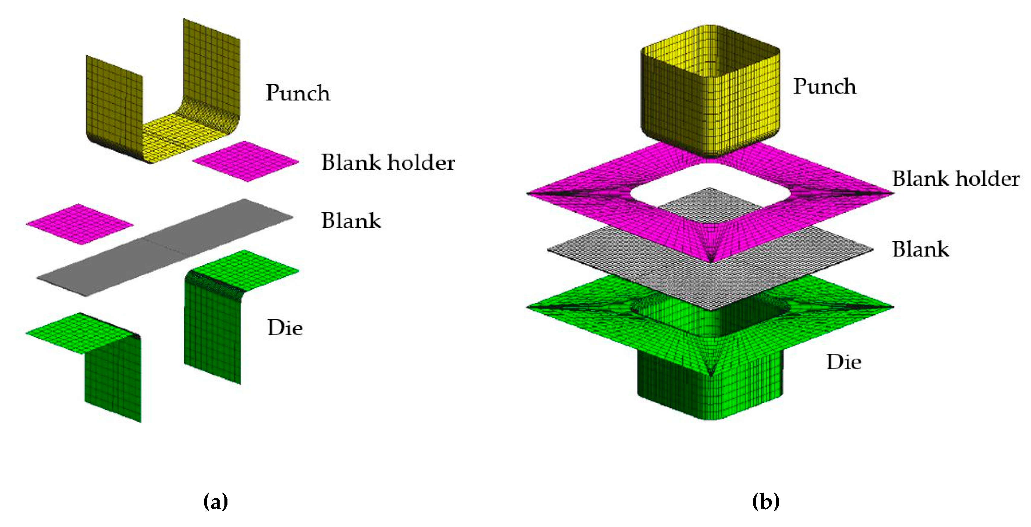
3.1. Numerical Models

The numerical models of the U-Channel and Square Cup forming processes are represented in Figure 1. Both processes comprise three main elements: the blank holder, the die, and the punch. The first stage of the forming process consists of reducing the distance between the die and the blank holder, until an imposed force is attained (blank holder force (BHF)). Then, the punch moves to promote the material flow into the die cavity, while the BHF remains constant. The U-Channel forming process ends after a total punch displacement of 30 mm, while the Square Cup forming process ends after a total punch displacement of 40 mm. The last stage consists of the tools removal, which promotes the recovery of the elastic energy stored in the part (springback). The initial dimensions of the blank of the U-Channel and the Square Cup forming processes are, respectively, 150 × 35 × 0.78 mm³ and 75 × 75 × 0.78 mm³. The material is considered orthotropic. Due to material and geometry symmetries, only one fourth of the blank is simulated for the Square Cup deep-drawing process, considering a finite element mesh with 1800, eight-node hexahedral solid elements. For the U-Channel, only half of the blank is considered, and boundary conditions are set to guarantee a plain strain state along the width of the blank, which enables the use of a total of 450, eight-node hexahedral solid elements.

The numerical simulations were carried out with the in-house finite element code DD3IMP, developed and optimized for simulating sheet metal forming processes [16]. The forming tool geometry was modeled using Nagata patches [17]. The contact with friction is described by Coulomb’s law with a constant value for the friction coefficient, µ, between the sheet and the tools. The constitutive model adopted in this study assumes (i) the isotropic elastic behavior described by the generalized Hooke’s law and (ii) the plastic behavior is anisotropic, as generally observed in metallic sheets, and as described by the orthotropic Hill’48 yield criterion combined with Swift isotropic hardening law. The Hill’48 yield criterion is described as follows:

$$F{\left({\sigma }_{yy}-{\sigma }_{zz}\right)}^2+G{\left({\sigma }_{zz}-{\sigma }_{xx}\right)}^2+H{\left({\sigma }_{xx}-{\sigma }_{yy}\right)}^2+2L{\tau }_{yz}^2+2M{\tau }_{xz}^2+2N{\tau }_{xy}^2=Y^2,$$

(10)

where ${\sigma }_{xx}$, ${\sigma }_{yy}$, ${\sigma }_{zz}$, ${\tau }_{xy}$, ${\tau }_{yz}$ and ${\tau }_{xz}$ are the components of the Cauchy stress tensor defined in the orthotropic coordinate system of the material; $F$, $G$, $H$, $L$, $M$ and $N$ are the anisotropy parameters and $Y$. is the flow stress. The condition $G+H=1$. is assumed and so $Y$. is represented by the uniaxial tensile stress along the rolling direction of the sheet. The parameters $L$ and $M$ are assumed equal to 1.5, as in isotropy (von Mises). The parameters $F$, $G$, $H$ and $N$ can be related with the anisotropy coefficients $r_0$, $r_{45}$ and $r_{90}$, as follows:

$$F=\frac{r_0}{r_{90}\left(r_0+1\right)}, G=\frac{1}{r_0+1}, H=\frac{r_0}{r_0+1}, N=\frac{1}{2}\frac{\left(r_0+r_{90}\right)\left(2r_{45}+1\right)}{r_{90}\left(r_0+1\right)}.$$

(11)

The Swift hardening law is expressed by:

$$Y=C{\left[{\left(Y_0/C\right)}^{\left(1/n\right)}+{\overline{\epsilon }}^p\right]}^n,$$

(12)

where ${\overline{\epsilon }}^p$ is the equivalent plastic strain and $C$, $Y_0$ and $n$ are material parameters. Two types of numerical simulation outputs were considered for each forming process: (i) springback and maximum thinning for the U-Channel process; and (ii) maximum equivalent plastic strain and maximum thinning for the Square Cup deep-drawing.

3.2. Parameter Variability

Three different steel grades were considered for each forming process: DC06, DP600, and HSLA340. For each of these materials, a normal distribution was assumed for describing the variability of the following inputs: $C$, $Y_0$ and $n$ of the Swift hardening law; Young’s modulus, E and Poisson coefficient ν of the generalized Hooke’s law; anisotropy coefficients $r_0$, $r_{45}$ and $r_{90}$; initial sheet thickness, $t_0$; and friction coefficient µ. The mean and standard deviation (SD) values of each parameter are detailed in

Table 1. Mean and standard deviation (SD) values for each input of the three materials considered [18].

Materials		C (MPa)	n	Y0 (MPa)	E (GPa)	ν	µ	r0	r45	r90	t0 (mm)
DC06	Mean	565.32	0.259	157.12	206	0.3	0.144	1.790	1.510	2.270	0.780
	SD	26.85	0.018	7.16	3.85	0.015	0.029	0.051	0.037	0.121	0.013
DP600	Mean	1093.0	0.187	330.30	210	0.3	0.144	1.010	0.760	0.980	0.780
	SD	52.46	0.02	9.64	7.35	0.015	0.029	0.04	0.03	0.06	0.01
HSLA340	Mean	673.0	0.131	365.30	210	0.3	0.144	0.820	1.070	1.040	0.780
	SD	32.30	0.011	10.67	7.35	0.015	0.029	0.033	0.039	0.061	0.005

. In addition to material parameters, the value of the BHF was also considered to introduce some variability in the process conditions; the mean and standard deviation values of the BHF for the U-Channel are 4900 N and 245 N, respectively; in the case of the Square Cup, the mean and standard deviation values of the BHF are 2450 N and 122.5 N, respectively.

3.3. Metamodel Generation and Evaluation

Based on the normal distribution of each input shown in Table 1, 1000 sets of inputs were randomly generated for each material. Numerical simulations of the U-Channel and Square Cup forming processes were performed for each of these randomly generated inputs, $\mathbf{x}$, with a total of 3 (materials) × 1000 (sets of inputs) = 3000 simulations for each forming process. For each material, the numerical simulations of each forming process were grouped into two sets: one training set, ${\mathbf{x}}^{\mathrm{t}}$, with 700 simulations used to generate the metamodels, and one testing set, ${\mathbf{x}}^{\mathrm{e}}$, with 300 simulations to evaluate the performance of the generated metamodels, by comparing the estimated/predicted output values with those obtained by numerical simulation. In addition to these sets, an extra training set and test set that includes simulations from all three materials was considered for each forming process. This was done to evaluate the impact of considering multiple materials on the predictive performance of the metamodels. The root mean square relative error (RMSRE) was used to evaluate the performance of each metamodel:

$$RMSRE=\sqrt{\frac{1}{l}{{\displaystyle \sum }}_{i=1}^l\left(\frac{{\mathrm{y}}_i\left(x^{\mathrm{e}}\right)-{\mathrm{y}}_i^{\ast }\left(x^{\mathrm{e}}\right)}{{\mathrm{y}}_i\left(x^{\mathrm{e}}\right)}\right)},$$

(13)

where $\mathrm{y}\left(x^{\mathrm{e}}\right)$ and ${\mathrm{y}}^{\ast }\left(x^{\mathrm{e}}\right)$ are the simulated and predicted response values for the set of testing inputs ${\mathbf{x}}^{\mathrm{e}}$, respectively, and $l$ is the number of testing points.

The parametric metamodels (RSM and PCE) where generated in Excel, while the ML metamodels where generated with python libraries, specifically, GPy [19] for the GP metamodels and Scikit-learn [20] for the remaining models.

4. Results and Discussion

Table 2. Values of root mean square relative error (RMSRE, %) obtained for the metamodel prediction for the U-Channel and Square Cup processes.

U-Channel	Springback				Maximum Thinning
	DC06	DP600	HSLA340	Mixed	DC06	DP600	HSLA340	Mixed
RSM	2.223	1.084	1.117	1.574	0.905	1.046	0.970	2.146
PCE	2.111	1.084	1.184	2.098	0.861	1.058	1.144	1.563
GP	2.132	1.060	1.023	1.572	0.849	1.025	0.875	1.017
MLP	1.986	1.113	1.019	1.476	0.772	1.242	0.782	1.097
SVR	2.230	1.056	1.090	1.538	0.883	1.048	0.864	1.083
DT	4.620	4.004	3.448	4.776	5.742	4.290	3.992	6.047
RF	2.876	2.726	2.298	3.545	4.022	2.815	2.796	4.104
kNN	4.068	3.777	2.950	4.542	10.846	5.599	5.585	6.877
KRR	2.168	1.057	1.072	1.546	0.851	1.035	0.865	1.060
Square Cup	Maximum Equivalent Plastic Strain				Maximum Thinning
	DC06	DP600	HSLA340	Mixed	DC06	DP600	HSLA340	Mixed
RSM	0.519	1.741	0.744	1.523	0.688	1.607	2.258	1.687
PCE	0.514	1.741	0.750	1.201	0.688	1.577	2.242	1.748
GP	0.493	1.618	0.666	1.230	0.672	1.538	2.195	1.529
MLP	0.607	1.653	0.952	1.416	0.661	1.553	2.233	1.633
SVR	0.533	1.606	0.836	1.231	0.688	1.585	2.221	1.556
DT	1.210	2.415	1.688	2.009	2.499	2.582	3.612	3.550
RF	0.823	1.830	1.308	1.490	1.734	1.850	2.682	2.527
kNN	1.322	2.754	2.253	2.899	2.481	2.419	3.084	4.188
KRR	0.518	1.689	0.665	1.321	0.673	1.545	2.147	1.532

Abbreviations: RSM, response surface method; PCE, polynomial chaos expansion; GP, Gaussian process; MLP, multi-layer perceptron, SVR, support vector regression; DT, decision tree; RF, random forest; kNN, k-nearest neighbors; KRR, kernel ridge regression.

presents the RMSRE values of the metamodels generated for each forming process (“U-Channel” and “Square Cup”), material (“DC06”, “DP600”, and “HSLA340”), and simulation output (“Springback”, “Maximum Thinning”, and “Maximum Equivalent Plastic Strain”); the results for the cases labeled as “Mixed” correspond to the metamodels generated from a training set that includes all three materials. The lowest value of RMSRE for each case, which corresponds to the best predictive performance, is highlighted.

The MLP model achieved the best performance in 6 of the 16 cases presented. For the remaining cases, the best performances were achieved by the GP (5), SVR (2), KRR (2), and PCE (1) models. It should be noted that the differences in performance between these five models were generally small. The RSM metamodels showed performances that were, in general, very similar to the PCE metamodels, and as such, can be considered as competitive with the models that achieved the best performances. On the other hand, the DT, RF, and kNN models performed clearly worse than the remaining metamodels for all cases. The few comparative studies found in the literature, namely Wessing et al. [5] and Ambrogio et al. [6], favored the use of the GP technique instead of ANN and RSM for thickness prediction, as it achieved significantly better results. In the current study, the GP technique also tended to present the best performance for the prediction of maximum thinning, but this was not valid for the other responses.

The inclusion of all three materials in the training and testing of the metamodels did not lead to significantly worse results, when compared to the performances obtained for the single material cases. In fact, in certain cases, the performance obtained for the models trained with the three materials surpassed the performance of models trained with just one material. For example, in the springback prediction for the U-Channel case, more than half of the metamodels tested achieved better performance when trained with the three materials than when trained specifically for the DC06 material. Thus, when training metamodels to predict forming process results considering various materials, it is worth considering the usage of just one dataset containing training data representative of all materials available, instead of training a different model for each material.

As an example, Figure 2 represents the comparison between the simulated values and the values predicted by the MLP and kNN algorithms for the testing dataset for the maximum thinning in the U-Channel process using DC06. The algorithms MLP and kNN were chosen for this comparison because they achieved the best and poorest performances, respectively, in this case.

Figure 3 presents the frequency distributions corresponding to the previous example, generated from 1000 new random points, according to the variability described in Table 1. The frequency distribution of the numerical simulation results is also represented and taken as a reference. The distribution obtained for the MLP metamodel closely resembles the distribution of the simulated results, however, the kNN shows more predictions in the range between 2.6% and 3.2%. In fact, the average value of the simulated results is 2.87%. This is in agreement with Figure 2b, where it is clear that the difference between predicted values and the corresponding simulated values is, in general, larger when the simulated values are further from the average.

5. Conclusions

In this work, parametric and non-parametric regression models were applied to predict the results of sheet metal forming processes, with the goal of evaluating their performance, and establish which metamodels offer the best results. It was concluded:

• The ML techniques can be divided into two groups in terms of performance:

  ○

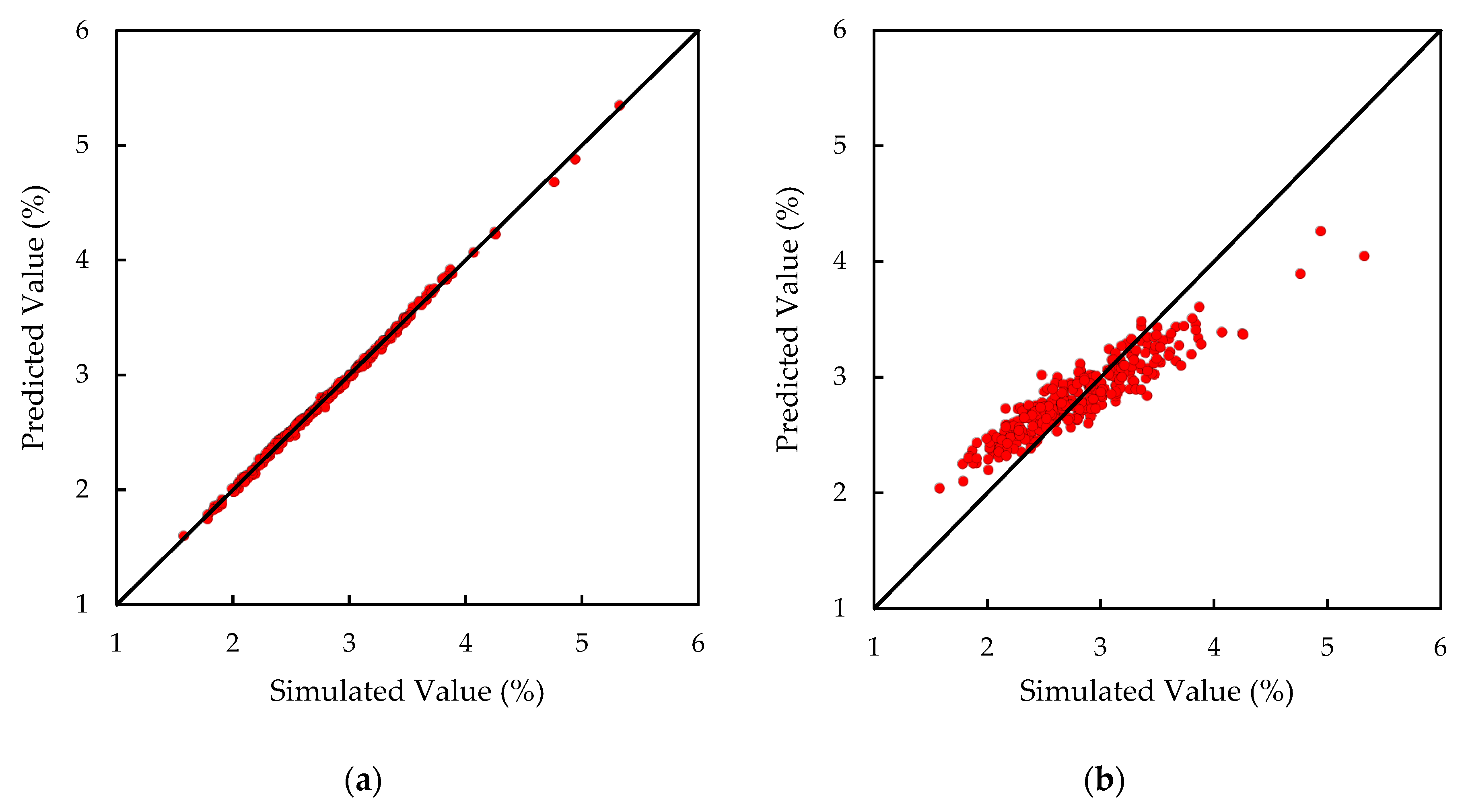
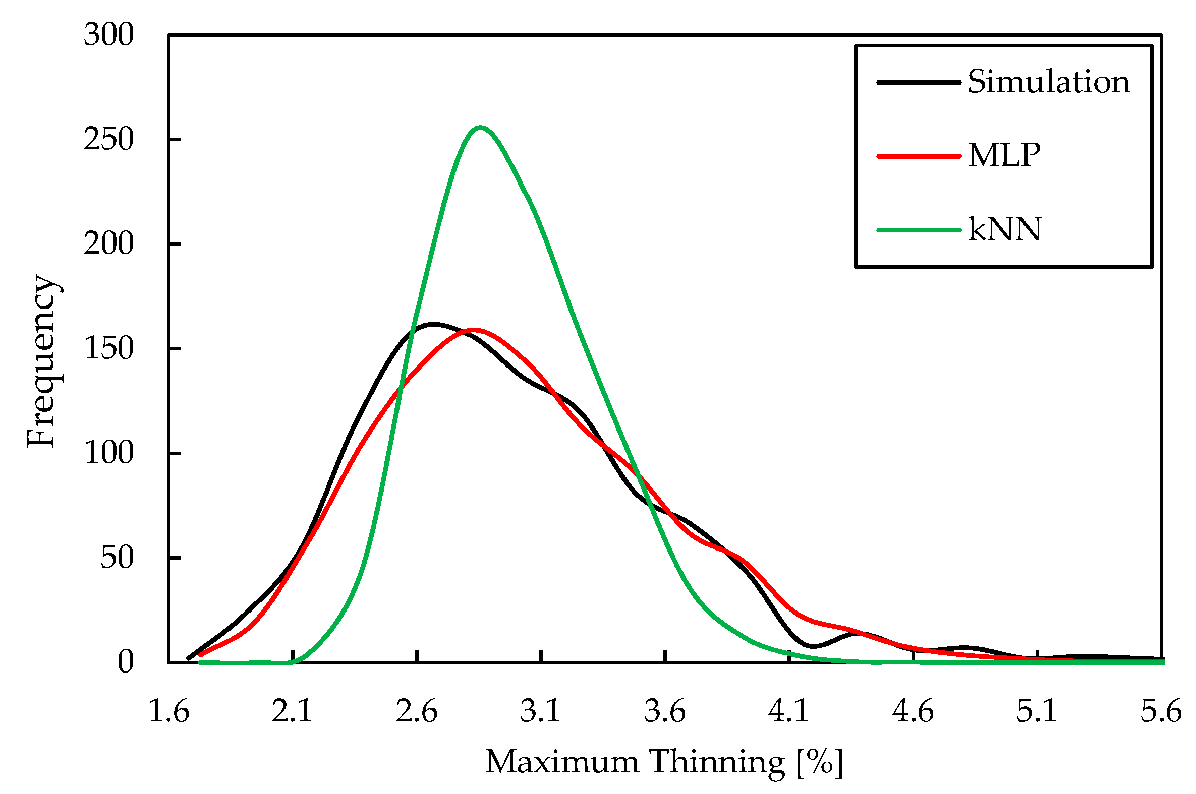
  The first group consists of the DT, RF, and kNN metamodeling techniques, which generally showed poor performances, with kNN in particular producing the poorest predictions.

  ○

  The second group consists of the MLP, GP, SVR, and KRR techniques. For almost all cases studied, the best predictive performance corresponded to one of these techniques, with MLP showing the best performance in more cases than any other. It is also of note that the performance of these techniques is comparable and, as such, the usage of any of them can be recommended.

• The parametric modeling techniques, RSM and PCE, showed competitive performances when compared with the second group of ML techniques and should be considered as valid alternatives.
• The performance of both types of modeling techniques depends on the response under analysis. For the particular case of the maximum thinning, GP shows better performance compared to the other techniques.
• When training metamodels to predict forming process results for different materials, the usage of just one dataset containing the training data of all materials should be considered, instead of training a different model for each material.

References

1. Wei, D.; Cui, Z.; Chen, J. Optimization and tolerance prediction of sheet metal forming process using response surface model. Comput. Mater. Sci. 2008, 42, 228–233. [Google Scholar] [CrossRef]
2. Naceur, H.; Ben-Elechi, S.; Batoz, J.L.; Knopf-Lenoir, C. Response surface methodology for the rapid design of aluminum sheet metal forming parameters. Mater. Des. 2008, 29, 781–790. [Google Scholar] [CrossRef]
3. Sun, G.; Li, G.; Li, Q. Variable fidelity design based surrogate and artificial bee colony algorithm for sheet metal forming process. Finite Elem. Anal. Des. 2012, 59, 76–90. [Google Scholar] [CrossRef]
4. Teimouri, R.; Baseri, H.; Rahmani, B.; Bakhshi-Jooybari, M. Modeling and optimization of spring-back in bending process using multiple regression analysis and neural computation. Int. J. Mater. Form. 2014, 7, 167–178. [Google Scholar] [CrossRef]
5. Wessing, S.; Rudolph, G.; Turck, S.; Klimmek, C.; Schäfer, S.C.; Schneider, M.; Lehmann, U. Replacing FEA for sheet metal forming by surrogate modeling. Cogent Eng. 2012, 1. [Google Scholar] [CrossRef]
6. Ambrogio, G.; Ciancio, C.; Filice, L.; Gagliardi, F. Innovative metamodelling-based process design for manufacturing: an application to Incremental Sheet Forming. Int. J. Mater. Form. 2017, 10, 279–286. [Google Scholar] [CrossRef]
7. Feng, Y.; Hong, Z.; Gao, Y.; Lu, R.; Wang, Y.; Tan, J. Optimization of variable blank holder force in deep drawing based on support vector regression model and trust region. Int. J. Adv. Manuf. 2019, 105, 4265–4278. [Google Scholar] [CrossRef]
8. Lin, J.D.; Huang, L.; Zhou, H.B. Forming defects prediction for sheet metal forming using Gaussian process regression. In Proceedings of the 29th Chinese Control and Decision Conference, Chongqing, China, 28–30 May 2017. [Google Scholar] [CrossRef]
9. Wiebenga, J.H.; Atzema, E.H.; An, Y.G.; Vegter, H.; van den Boogaard, A.H. Effects of material scatter on the plastic behavior and stretchability in sheet metal forming. J. Mater. Process. Technol. 2014, 214, 238–252. [Google Scholar] [CrossRef]
10. Blatman, G. Adaptive Sparse Polynomial Chaos Expansions for Uncertainty Propagation and Sensitivity Analysis. Ph.D. Thesis, Université Blaise Pascal, Clermont-Ferrand, France, 8 October 2009. [Google Scholar] [CrossRef]
11. Kaur, D.; Wilson, D.; Forrest, M.; Feng, L. Regression tree and neuro-fuzzy approach to system identification of laser lap welding. In Proceedings of the 2005 Annual Meeting of the North American Fuzzy Information Processing Society, Detroit, MI, USA, 26–28 June 2005. [Google Scholar] [CrossRef]
12. Segal, M.R. Machine Learning Benchmarks and Random Forest Regression. In UCSF: Center for Bioinformatics and Molecular Biostatistics; 2004; Available online: https://escholarship.org/uc/item/35x3v9t4 (accessed on 30 January 2020).
13. Cook, B.; Huber, M. Balanced k-Nearest Neighbors. In Proceedings of the Thirty-Second International Flairs Conference, Florida, FL, USA, 19–22 May 2019. [Google Scholar]
14. Smola, A.J.; Schölkopf, B. A tutorial on support vector regression. Stat. Comput. 2004, 14, 199–222. [Google Scholar] [CrossRef] [Green Version]
15. Welling, M. Kernel ridge regression. Max Welling’s Classnotes in Machine Learning. 2013. Available online: https://www.ics.uci.edu/~welling/classnotes/papers_class/Kernel-Ridge.pdf (accessed on 30 January 2020).
16. Menezes, L.F.; Teodosiu, C. Three-dimensional numerical simulation of the deep-drawing process using solid finite elements. J. Mater. Process. Technol. 2000, 97, 100–106. [Google Scholar] [CrossRef] [Green Version]
17. Neto, D.M.; Oliveira, M.C.; Menezes, L.F. Surface Smoothing Procedures in Computational Contact Mechanics. Arch. Comput. Meth. Eng. 2017, 24, 37–87. [Google Scholar] [CrossRef]
18. Alves, J.L. Simulação Numérica do Processo de Estampagem de Chapas Metálicas. Ph.D. Thesis, University of Minho, Guimarães, Portugal, 7 November 2003. [Google Scholar]
19. GPy: A Gaussian Process Framework in Python. Available online: http://github.com/SheffieldML/GPy (accessed on 22 January 2020).
20. Pedregosa, F.; Varoquaux, G.; Gramfort, A.; Michel, V.; Thirion, B.; Grisel, O.; Blondel, M.; Prettenhofer, P.; Weiss, R.; Dubourg, V.; et al. Scikit-learn: machine learning in python. J. Mach. Learn. Res. 2011, 12, 2825–2830. [Google Scholar]
Figure 1. Representation of the finite element models for the (a) U-Channel; (b) Square Cup.
Metals 10 00457 g001
Figure 2. Comparison between simulated and predicted values of maximum thinning in the U-Channel case with the DC06 material by the algorithms: (a) MLP; (b) kNN.
Metals 10 00457 g002
Figure 3. Frequency distributions obtained for the numerical simulations and predictions by the MLP and kNN algorithms, considering the maximum thinning in the U-Channel case with the DC06 material.
Metals 10 00457 g003