Interfacial Fracture Toughness Assessment of a New Titanium–CFRP Adhesive Joint: An Experimental Comparative Study


1
Laboratory of Applied Mechanics and Vibrations, Department of Mechanical Engineering and Aeronautics, University of Patras, GR-26504 Rio-Patras, Greece
2
Structures Technology Department, Royal Netherlands Aerospace Centre NLR, 8316 PR Marknesse, The Netherlands
*
Author to whom correspondence should be addressed.
Metals 2020, 10(5), 699; https://0-doi-org.brum.beds.ac.uk/10.3390/met10050699
Submission received: 24 April 2020
/
Revised: 13 May 2020
/
Accepted: 15 May 2020
/
Published: 25 May 2020
(This article belongs to the Special Issue Recent Advances in Fibre Metal Laminates)
Abstract
:Adhesive joints between dissimilar layers of metals and composites are increasingly used by different industries, as they promise significant weight savings and, consequently, a reduction in energy consumption and pollutant emissions. In the present work, the interfacial fracture behavior of a new titanium–carbon fiber reinforced plastic (CFRP) adhesive joint is experimentally investigated using the double cantilever beam (DCB) and end-notched flexure (ENF) test configurations. A potential application of this joint is in future large passenger aircraft wings. Four characteristic industry relevant manufacturing approaches are proposed: co-bonding with/without adhesive and secondary bonding using thermoset/thermoplastic CFRP. For all of them, the vacuum-assisted resin transfer molding (VARTM) technique is utilized. To prevent titanium yielding during testing, two aluminum backing beams are adhesively bonded onto the primary joint. A data reduction scheme recently proposed by the authors, which considers effects such as bending–extension coupling and manufacturing-induced residual thermal stresses, is utilized for determination of the fracture toughness of the joint. The load–displacement responses, fracture behaviors during testing, and fracture toughness performances of the four manufacturing options (MOs) under consideration are presented and compared.
1. Introduction
The development of lightweight materials and structures is a target for a number of different industries, including aerospace, automotive, and wind energy. This area of study promises significant weight savings and, subsequently, a reduction in energy consumption and pollutant emissions. Dissimilar adhesive joints are a class of structural elements that, as is widely known, can decisively contribute towards this goal. Thus, there has been a significantly increased use of dissimilar adhesive joints in recent decades.
By definition, a dissimilar adhesive joint is created by the adhesive joining of two or more materials with different mechanical/physical properties and/or thicknesses. Aluminum, titanium, steel, and carbon or glass fiber/epoxy composites are some of the materials most often chosen by the industries that develop dissimilar adhesive joints. When the application requires them, high-performance adhesives that are polymerized at high temperatures are used, inevitably generating residual thermal stresses in the joint. Consequently, for the design and analysis of a dissimilar adhesive joint, one has to consider not only the different mechanical properties, physical properties, and thicknesses of the joint’s adherents but also the effect of residual thermal stresses. In fact, for fracture toughness, which is a critical property to be determined in the design of a new dissimilar joint, certain studies (e.g., [1,2]) indicate a significant effect of residual thermal stresses.
Most of the published literature on the mixed-mode fracture of dissimilar adhesive joints is interested in adhesive joints consisting of two adherents that are either isotropic or “homogeneous” (i.e., without elastic couplings), see e.g., [3,4,5,6]. Typical examples of such joints are metal–composite joints, where the metal is obviously an isotropic layer and the composite laminate typically is unidirectional, quasi-isotropic or, in general, it does not present any elastic coupling (e.g., bending–extension coupling, etc.).
There is only a small group of published works that investigate the interfacial fracture of joints (or, to be more precise, multi-layered beam-like specimens) consisting of two “non-homogeneous” (i.e., elastically coupled) sub-laminates [7,8,9,10,11,12,13,14]. In this case, studying the various published papers [7,8,9,10,11,12,13,14], we observed that the experimental data were post-processed using different data reduction approaches, from simpler approaches, such as the Euler beam theory or William’s global method, to more sophisticated ones, such as Wang and Qiao’s [15] approach. In some cases, the utilized data reduction scheme does not consider the elastic coupling effects and thus does not give accurate predictions of the fracture toughness.
In [7], doubler plates were adhesively bonded to delaminated specimens of a thin composite to prevent bending failure of the unbonded arms of the specimen. The data reduction equations for some common test configurations were re-derived for use with specimens that have bonded doublers. In [8], an experimental approach for obtaining the critical mode I and II strain energy release rates (SERRs) for interfacial fracture in a sandwich composite was outlined. By modifying the geometry of the sandwich beam such that the crack plane and neutral axis coincide, mode I and II SERRs were respectively obtained by double cantilever beam (DCB) and end-notched flexure (ENF) tests. The geometry modification required that the bending stiffnesses of the two arms of the beam be equal. In [9], a semi-analytical methodology was proposed to predict fracture behavior under a mixed-mode bending test of asymmetric glass fiber reinforced plastic adhesive joints. The main advantage of this methodology is the ability to consider the fiber bridging effect and the arbitrariness of the adherents’ stacking sequences. In [10], multi-directional fiber metal laminates were subjected to ENF tests. A methodology was then proposed to obtain the SERR and the mode mixity using an enhanced beam theory-based analytical model, which was validated by the standardized compliance calibration method. In [11], plate theory analyses were employed to obtain the SERR and the mode mixity of DCB tests on carbon fiber aluminum laminates, which were compared with the compliance calibration method’s predictions. The SERRs acquired by both methods were identical for the initial crack length, but by increasing the crack length, the fracture energies estimated by the plate theory surpassed those by the compliance calibration method. In [12], the mode I fracture toughness of the metal/composite interface region of some fiber metal laminates were determined and a finite element model was developed to account for the influence of metal plasticity on the measured fracture toughness. In [13], modified DCB specimens were tested to investigate the mode I fracture properties of an asymmetric metal–composite adhesive joint. A modified form of Kanninen’s theory, capable of considering the specific specimen design, was then used. In [14], the interlaminar fracture toughness of some glass laminate aluminum reinforced epoxy (GLARE) laminates was investigated by simple but approximate beam theory-based and fracture mechanics-based analytical solutions.
In the realm of adhesively bonded joints, the vast majority of literature focuses on similar adhesive joints and addresses issues related to the development, evaluation, and utilization of experimental techniques for the characterization of these joints. Among these studies, only a few (see, for example, [16,17]) attempt to compare two of the most common industrial techniques for the manufacturing of composite–composite or metal–composite adhesive joints—i.e., co-bonding and secondary bonding techniques.
In summary, experimental works on the interfacial fracture toughness of dissimilar and multi-layered metal–composite adhesive joints are rare [7,8,9,10,11,12,13,14]. Works comparing the fracture toughness of joints manufactured by different industrial technologies are also very uncommon [16,17].
The present paper presents results from a systematic experimental investigation of the quasi-static mode I and mode II interfacial fracture toughness of adhesively bonded joints between titanium and carbon fiber reinforced plastic (CFRP) using the DCB and ENF test configurations. This work builds upon previous research by the research groupon the same topic [18,19,20,21,22]. This paper is an extension of two previous preliminary studies by the authors and co-workers that were recently presented at conferences and published in conference proceedings [21,22]. The aim of the present paper is, therefore, to present more enriched, complete, results from our study and discuss them.
As a requirement for the intended industrial application of the present joint (more information on this application is available in [18]), the two adherents (titanium and CFRP) must be thinner than 1.5 mm. Issues related to the design of interfacial fracture toughness tests (i.e., DCB and ENF tests) on the present adhesive joint were covered in a previous paper [19] by our group, while the results from a study on the fatigue fracture performance of the present joint may be found in [20].
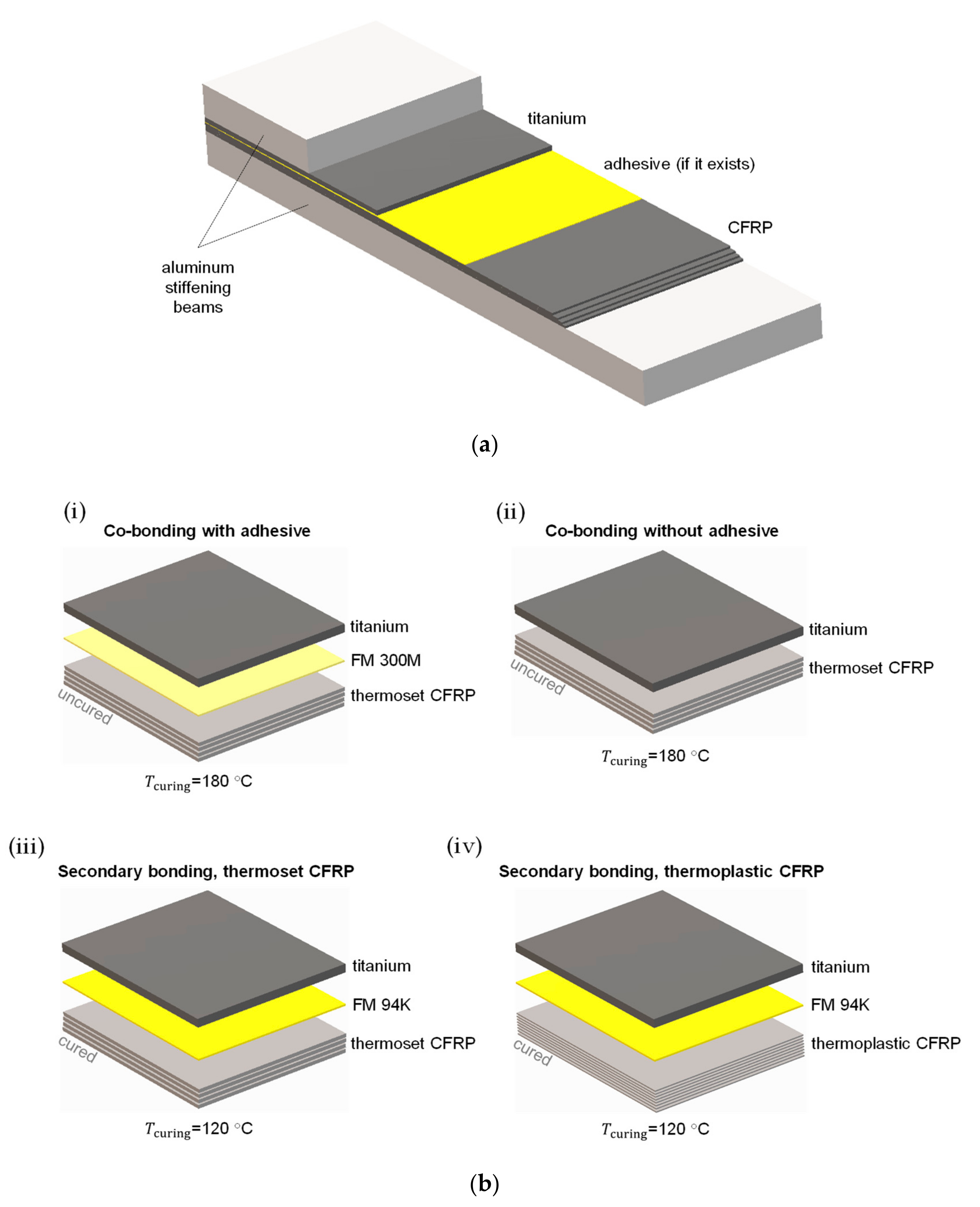
The present work focuses on comparing four representative industry relevant options for the manufacturing of a bonded joint in terms of its interfacial fracture toughness. For each manufacturing option (MO), a combination of different composite materials (thermoset CFRP and thermoplastic CFRP), adhesive agents, and/or bonding techniques was utilized. After the production stage and cutting of the panels into test specimens, due to the small thickness of the adherents, the joints needed to be stiffened, as schematically presented in Figure 1a, following the procedures reported in [19]. As a consequence, bending–extension coupling effects were introduced. Following all MOs, the high-temperature manufacturing process created non-negligible residual thermal stresses. Investigation of the interfacial fracture toughness of the joint was performed following quasi-static DCB and ENF experiments, after which fractographic studies took place. The application of a recently published [2] data reduction scheme for calculating the fracture toughness of the joint is believed to be an interesting aspect of the present work. This data reduction scheme, in contrast to the state-of-the-art data reduction schemes used for experimental data reduction (such as the data reduction schemes referenced in the Introduction), can take into account both bending–extension coupling (through the presence of stiffening beams) and residual thermal stresses (as a result of high-temperature manufacturing) effects.
The contributions of the present work can be outlined as follows:
- A novel, aerospace grade, adhesive joint between titanium and CFRP that was bonded using epoxy-based adhesive film was successfully manufactured and systematically characterized using interfacial fracture toughness experiments.
- Four characteristic high-end manufacturing approaches, including co-bonding and secondary bonding, using different composite materials, adhesive agents, and adhesive curing temperatures were compared in terms of their interfacial fracture performance.
- A data reduction scheme recently proposed by a sub-set of the present authors [2] was applied to the post-processing of the experimental data. This data reduction scheme is able to consider the two main peculiarities of the joint: bending–extension coupling and residual thermal stresses effects.
- A systematic fractographic investigation under an optical microscope was applied to cast light on the involved fracture processes.
The structure of the paper is as follows. Section 2 presents the geometry of the joint under study, the materials used and the manufacturing processes applied, the methods for the execution of the experiments, and the methodology applied for the fractographic analysis. The section ends with a brief presentation of the analytical model [2] used for experimental data reduction. Section 3 presents the results from the present DCB and ENF experiments, i.e., the load–displacement responses, the fracture behaviors during testing, and the fracture toughness performances. Section 4 summarizes the conclusions of the work.
2. Materials and Methods
2.1. The Titanium–CFRP Adhesive Joint
The joint under study [18,19,20,21,22] is schematically defined in Figure 1a. It consists of two thin adherents, one 0.8-mm-thick titanium sheet and a CFRP laminate with a thickness of approximately 1.5 mm. As previously noted, the high-temperature curing of the adhesive joint generates residual thermal stresses. Two 5-mm-thick aluminum beams were also used as stiffening elements [19]. For the adhesive agent, three different options were examined, as described in the next paragraph.
2.2. The Proposed Manufacturing Options (MOs)
For the purpose of the present work, we have chosen to evaluate/compare the following four MOs:
- MO 1: “Co-bonding with adhesive” (Figure 1b-i). Titanium and thermoset CFRP are co-bonded using an FM 300M film adhesive (Solvay Composite Materials, Tempe, AZ, USA), followed by vacuum infusion/resin transfer molding (RTM) (at 180 °C).
- MO 2: “Co-bonding without adhesive” (Figure 1b-ii). Titanium and thermoset CFRP are co-bonded without using any adhesive, followed by vacuum infusion/RTM (at 180 °C). In this MO, the excess HexFlow RTM6 epoxy resin (Hexcel Corporation, Stamford, CT, USA) of the CFRP is utilized for bonding.
- MO 3: “Secondary bonding, thermoset CFRP” (Figure 1b-iii). The thermoset CFRP is cured by vacuum infusion/RTM. Next, the titanium and thermoset CFRP are secondarily bonded using an FM 94K film adhesive (Solvay Composite Materials, Tempe, AZ, USA), followed by autoclave curing (at 120 °C).
- MO 4: “Secondary bonding, thermoplastic CFRP” (Figure 1b-iv): The thermoplastic CFRP is manufactured using fiber placement and autoclave curing techniques. Next, the titanium and thermoplastic CFRP are secondarily bonded using an FM 94K film adhesive, followed by autoclave curing (at 120 °C).
The proposed MOs are some of the industry’s most typical options for production of metal–composite (or, of course, composite–composite) adhesive joints. The co-bonding approach (i.e., MOs 1 and 2) simplifies the manufacturing process and is more advanced than the secondary bonding approach (i.e., MOs 3 and 4), but it is less mature in the aerospace industry. MO 2 is considered more advanced than MO 1 since the former uses no adhesive. MO 3 is a low-risk MO that uses proven, existing technologies. Compared to all previous MOs, MO 4 is more appropriate for the manufacturing of corrugated structures since the press forming of hat stringers of carbon fiber/polyetherketoneketone (PEKK) composites is simpler than using vacuum infusion/RTM.
Throughout the paper, we refer to the MO 2 joint as an “adhesive joint”, assuming that the matrix material of the CFRP, i.e., the RTM6, plays the role of an adhesive in the interface between the titanium and CFRP.
2.3. Materials
The materials utilized in the present work are summarized below:
- Titanium CP40, Material AMS4902, Grade 2 (Salomon’s Metalen, Groningen, The Netherlands) with the rolling direction parallel to the length direction of the resulting test specimens.
- For the thermoset CFRP: HexFlow RTM6 epoxy resin and 5-harness weave fabric Hexforce G0926 (Hexcel Corporation, Stamford, CT, USA) with a 6K HS carbon fiber and an areal weight of 370 gsm.
- For the thermoplastic CFRP: Cetex TC1320 PEKK (Toray Advanced Composites, Morgan Hill, CA, USA) with an AS4D fiber and an areal weight of 145 gsm.
- Aluminum 2024 T3 (Salomon’s Metalen, Groningen, The Netherlands).
- Adhesives: (a) FM 300M 0.03 psf adhesive film with a mat carrier, an areal weight equal to 150 gsm, and a nominal thickness equal to 0.13 mm. (b) FM 94K 0.06 psf adhesive film with a knit carrier, an areal weight equal to 293 gsm, and a nominal thickness equal to 0.25 mm.
For the bonding of the aluminum backing beams and for the artificial starter crack, the following materials were also used:
- 3M Scotch-Weld 9323 B/A adhesive (3M, St. Paul, MN, USA) with a nominal thickness equal to 0.20 mm.
- Upilex-25S foil (Airtech, Niederkom, Luxembourg) with a thickness equal to 0.025 mm.
The thermoset and thermoplastic CFRPs consist of four woven layers and eight unidirectional layers, respectively, while their stacking sequences are [0°/45°]s and [0°/45°/90°/−45°]s, respectively. In other words, both chosen CFRP laminates are quasi-isotropic, thereby providing excellent resistance to impact damage. Such stacking sequences are frequently used on the leading edges of aircraft [18].
For the needs of the present work, we utilized two typical and aerospace grade epoxy-based adhesives—FM 300M and FM 94K adhesives. We used two different adhesives because the two different joining techniques applied (co-bonding and secondary bonding) require different curing temperatures. To be specific, for the co-bonding, we preferred to use an adhesive with a curing temperature similar to that of the CFRP (180 °C). For secondary bonding, we preferred to use an adhesive with a relatively low curing temperature (in our case, 120 °C) to minimize the residual thermal stresses induced by the curing process.
In Table 1, the material properties and thicknesses of the utilized materials are summarized.
2.4. Manufacturing Processes and Preparation of the Test Specimens
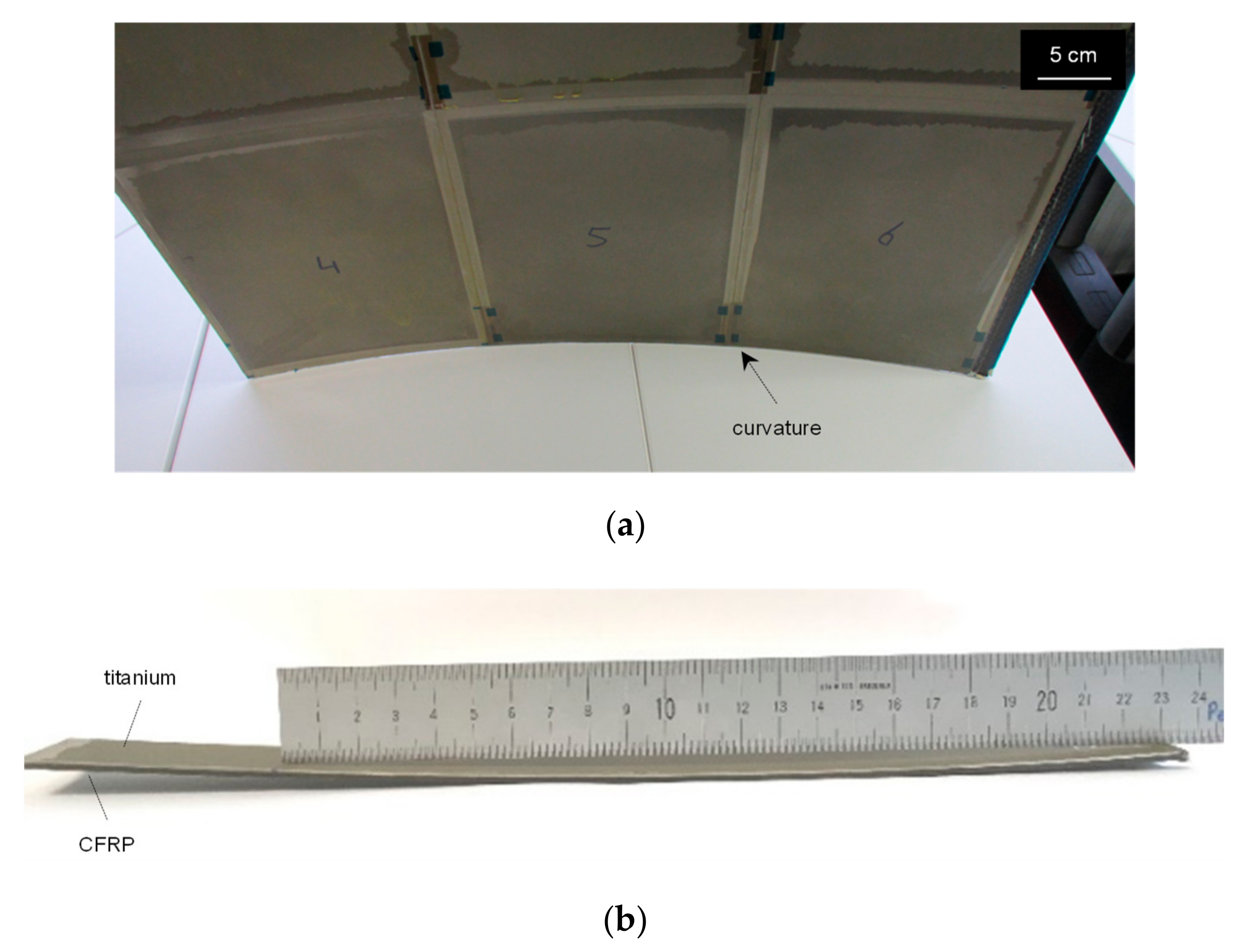
All issues related to the manufacturing processes and, subsequently, the preparation of the test specimens are detailed in [21] (pp. 3–4). After the manufacturing stage, the resulting panels from all MOs appeared to be curved as a result of the different coefficients of thermal expansion (CTEs) of the adherents and the high curing temperature applied (120 °C or 180 °C, depending on the MO). Figure 2 clearly depicts this curvature.
2.5. Mechanical Experiments
To determine the quasi-static mode I and II interfacial fracture toughness of the titanium–CFRP joint, DCB and ENF experiments were performed on an Instron 8872 universal testing machine (Instron, High Wycombe, UK) with a 25 kN axial force capacity. The DCB and ENF experiments were conducted in general alignment with the guidelines of the ASTM D 5528-01 and AITM 1.0006 test standards, respectively. All tests were performed under room temperature conditions (i.e., temperature of 25 °C and relative humidity of 50–60%).
2.5.1. Double Cantilever Beam (DCB) Experiments
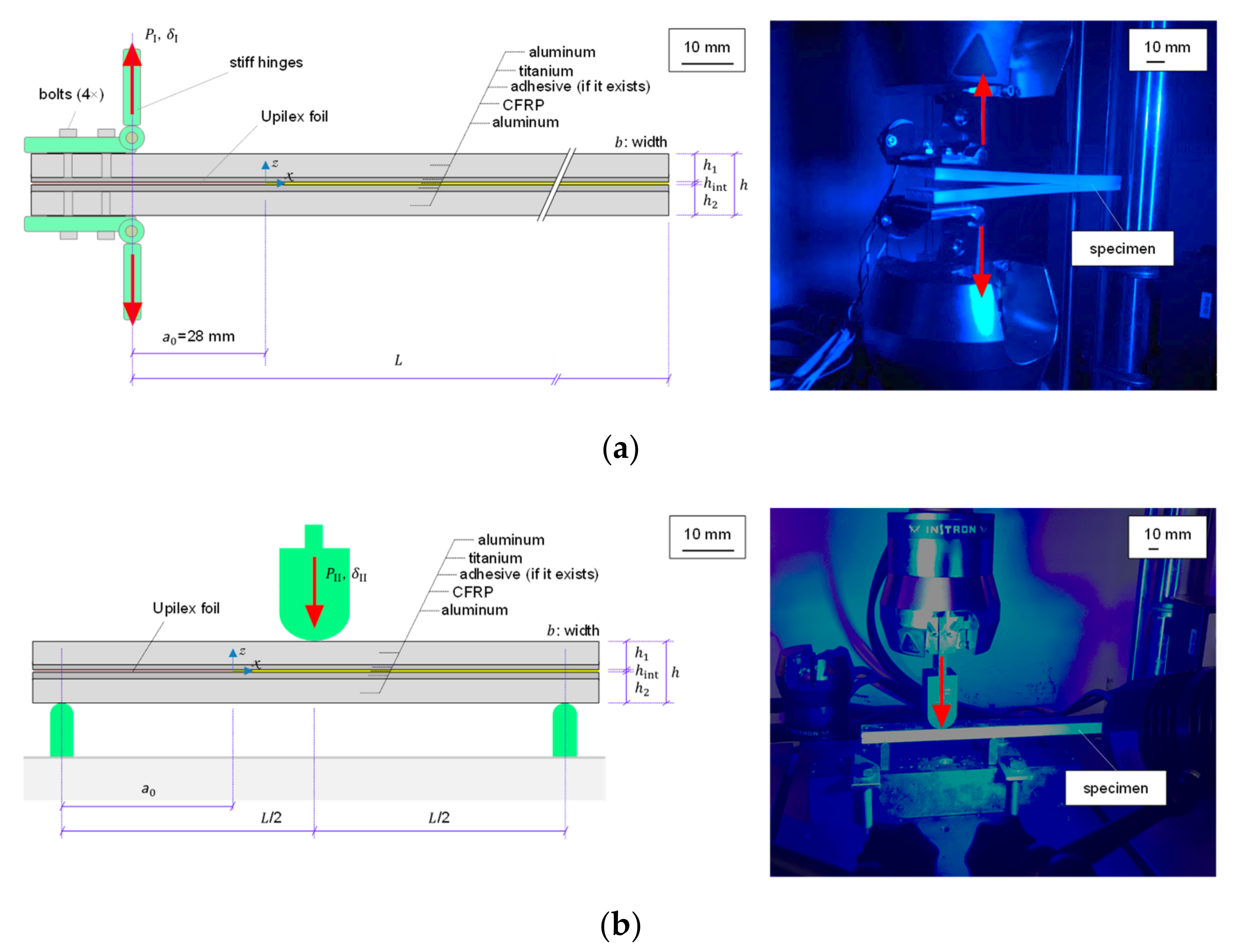
Figure 3a presents a sketch of the DCB experimental setup, whose basic dimensions are the width , the total length , the initial crack length , and the sub-laminate thicknesses and . The actual values of these dimensions are given in Table 2. Figure 3a shows the position of the Upilex starter film, which was placed in the titanium/CFRP interface. is the thickness of the interface layer. As the sketch of Figure 3a shows (and as can be seen in the photograph of the right part of the same figure), for the present DCB tests, we utilized piano hinges that are stiffer than those that a typical DCB test requires since the loading values during the tests were high.
As presented in Table 2, the starting crack length was not equal for all specimens from different MOs. We originally aimed to create a natural crack prior to the test because a natural crack has a sharp crack tip, thereby leading to more representative fracture toughness values compared to starter films that introduce blunt crack tips. However, in MOs 1 and 3, when we attempted to form a natural crack, we always ended up with delamination inside the composite adherent. Consequently, we chose to start the test from the artificial pre-crack ( = 28.0 mm).
Regarding the MO 2 specimens, each test was performed in two steps. First, mode I loading was applied to open the crack until reached the target value of about 70 mm, followed by unloading. Then, the actual mode I test commenced until the crack progressed to an extra length of approximately 40 mm. For the MO 4 specimens, wedge loading was first applied to the specimens to create a natural pre-crack. The new initial crack length (i.e., the length from the loading axis to the tip of the natural crack) was measured and was used in the post-processing of the experimental data (see Section 2.7). Because wedge loading is less controllable, it was not easy to control the propagated crack length. Thus, the four MO 4 specimens have quite different values, as reported in Table 2.
The right part of Figure 3a shows a snapshot during one typical DCB experiment. During each experiment, the specimen was loaded under tension (i.e., the crack tip was loaded in mode I) at a constant displacement rate of 10 mm/min. A high-resolution digital camera was used to capture the crack initiation. For the output, we took continuous recordings of the load () and load-point displacement (). The resulting load–displacement curves from 14 valid experiments were registered and used as the starting point to evaluate the mode I fracture behavior of the joint.
2.5.2. End-Notched Flexure (ENF) Experiments
Figure 3b depicts the experimental setup of the ENF tests. Here, the dimensions of width , span length , and the initial disbond length are shown, while their actual values are listed in Table 2. The span length of the MO 2 specimens is shorter than that of the rest of the specimens because the tests were performed by two different institutions. More specifically, ΜO 1, 3, and 4 were tested by the University of Patras, Greece, whereas MO 2 was tested in another test fixture at NLR, The Netherlands. The thicknesses of the two sub-laminates, and , are also given in Table 2. In the ENF tests, based on previous experience with DCB tests, we directly started the test from the artificial crack (i.e., = 35 mm for all ENF experiments) without trying to create a natural crack.
The right part of Figure 3b shows a snapshot during one of the ENF tests. During each experiment, the load () was continuously applied to the specimen through a three-point bending setup, with a constant displacement rate of 1 mm/min. A camera was also used to monitor the crack tip and capture the crack initiation. The test stopped just after the first major load drop. At least three specimens from each MO were tested. The obtained sets of load–displacement curves were used to characterize the mode II fracture performance of the joint.
2.6. Fractographic Investigation
After the tests, the two sub-laminates of some DCB and ENF specimens were completely separated, and their fracture surfaces and longitudinal sections (side-views) were observed using a digital camera. They were then further inspected under an optical microscope. This investigation helped shed light on the fracture mechanisms and draw some qualitative conclusions about the qualities of the four MOs.
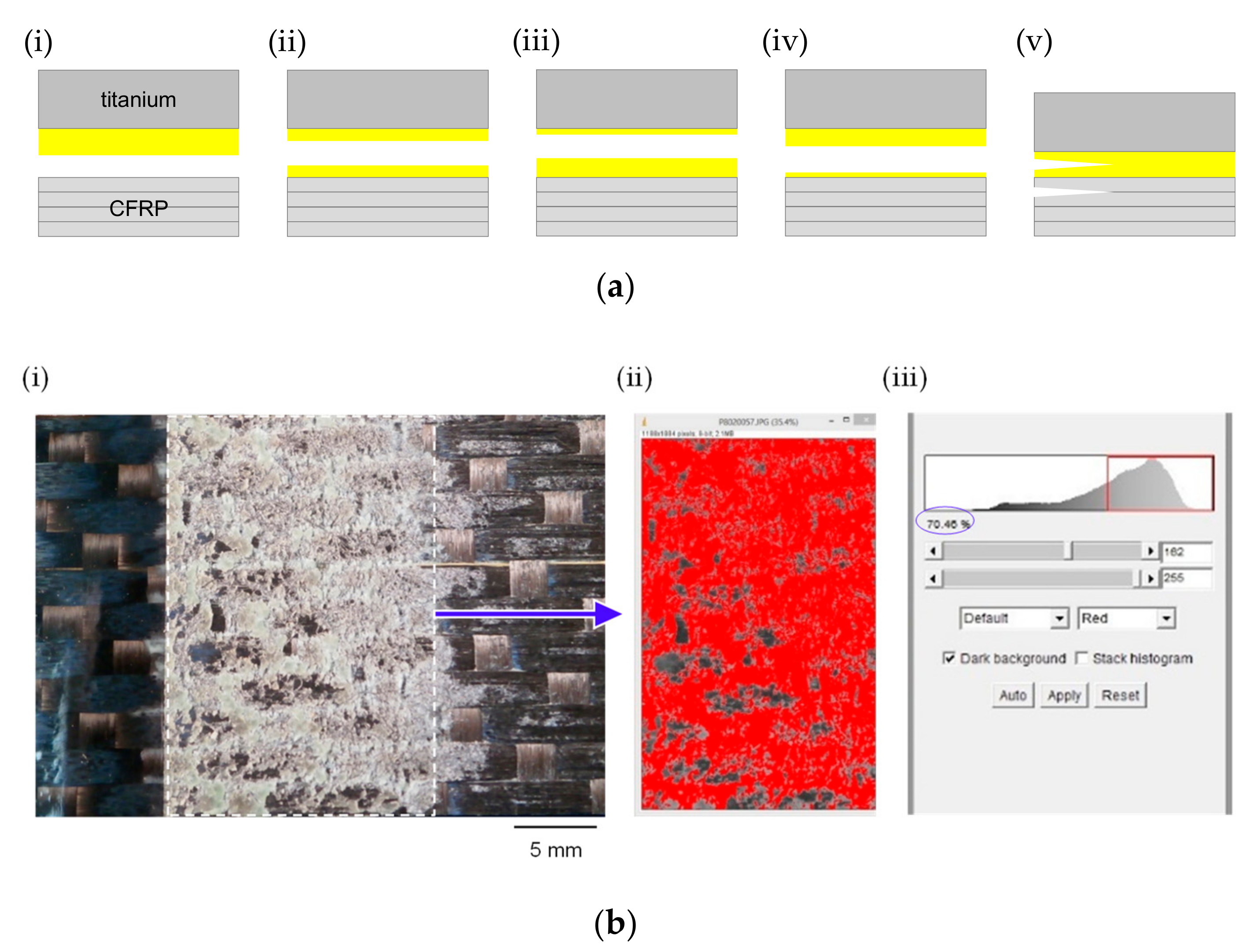
First, the two fracture surfaces of each specimen were inspected visually and via macro-photographs recorded using a high-resolution digital camera to identify all possible failure modes. According to the ASTM D5573 standard, the possible failure modes for adhesive joints between fiber reinforced plastics are “adhesive failure”, “cohesive failure”, “thin-layer cohesive failure”, “fiber-tear failure”, “light-fiber-tear failure”, “stock-break failure”, “adhesive to adhesion promoter”, and “adhesion promoter to substrate”. We adapted this classification here since no standard classification of the failure modes of adhesive joints between metals and composites currently exists. The principal failure modes we observed in the present work (schematically presented in Figure 4a) are classified as follows: FM1, adhesive failure (Figure 4a-i); FM2, cohesive failure (Figure 4a-ii); FM3, thin-layer cohesive failure, titanium side (Figure 4a-iii); FM4, thin-layer cohesive failure, CFRP side (Figure 4a-iv); and FM5, adherent failure (Figure 4a-v). As discussed in the next section, the “adherent failure” observed here is the delamination between the first and second composite layers, occurring in combination with interfacial failure.
Next, for each of the above failure modes, we determined the failure mode percentage after the DCB and ENF tests. We recall that the failure mode percentage is defined as the surface area occupied by one given failure mode, divided by the total surface area. We applied the following simple procedure (Figure 4b). First, we took a picture from each fracture surface (of the titanium and CFRP sides) using a high-resolution digital camera (Figure 4b-i). Next, we processed these pictures using the ImageJ (NIH, Maryland, MD, USA) image processing software (Figure 4b-ii). In the example fracture surface of Figure 4b-ii, the areas of the fracture surface featuring a thick layer of adhesive on the composite side’s fracture surface are colored in red. This percentage is equal to 70.5% in the paradigm of Figure 4b, as Figure 4b-iii suggests. Based on this simple procedure, the failure mode percentages were deduced and are presented in Section 3.
Using some of the fractured ENF specimens, samples were cut using a waterjet cutter to investigate their side-views under an optical microscope. All samples were extracted from the portion of each specimen where the crack propagation took place. After cutting, the samples were retained using small firs and were embedded in a polymer-based mounting agent, followed by polishing of the surfaces under examination. The examinations were performed using a Sinowon IMS-300 inverted metallurgical microscope (Sinowon, Dongguan, China).
2.7. Experimental Data Reduction
2.7.1. Determination of the Crack Initiation Load
As detailed later, we observed unstable crack propagation combined with multiple cracking phenomena in all DCB experiments presented here (see Section 3.1.1). Thus, only the initiation fracture toughness (i.e., the total SERR and mode mixity at the crack initiation load), but not the propagation toughness or the crack growth resistance (-) curve, was determined in the present work.
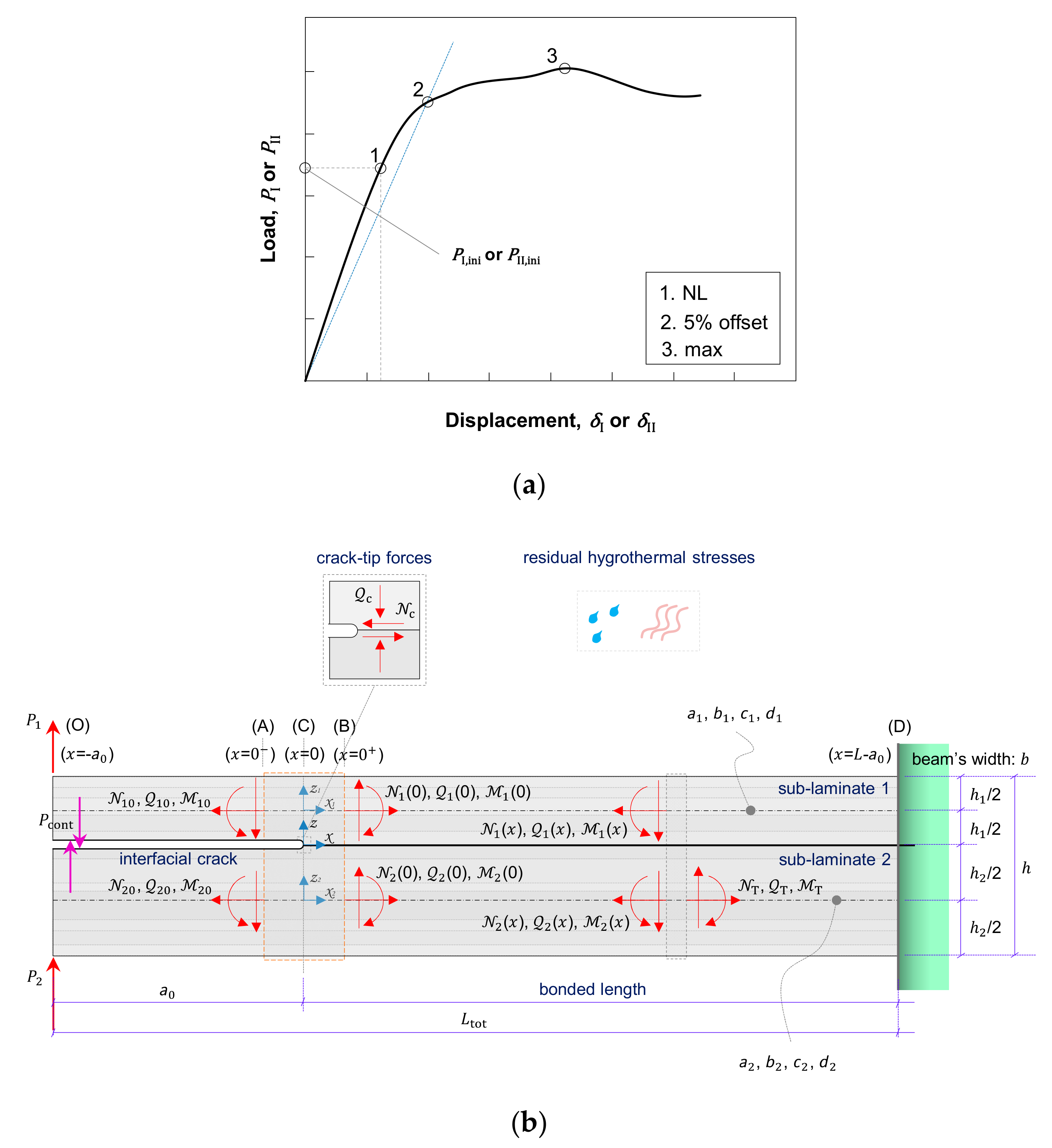
To determine the crack initiation load, the ASTM D5528 standard defines three criteria that are commonly used: (a) the “deviation from linearity” (NL), (b) the “visual observation” (VIS), and (c) the “5% offset/maximum load” (5%/max) (Figure 5a).
In the present work, to estimate the , the NL criterion was followed. In the DCB tests, both the NL and the 5%/max criteria gave identical values. In the ENF tests, where the determination of the crack initiation point () was difficult, we estimated the by taking into consideration the predictions by both the VIS (based on videos of the crack-tip’s movement taken using a high-resolution camera) and the NL criteria. Nevertheless, in some of the ENF experiments, the camera was not able to reliably capture the crack initiation point, so these experiments were considered invalid.
2.7.2. Determination of the Total Strain Energy Release Rate (SERR) and Mode Mixity
As already discussed, the DCB and ENF specimens shown in Figure 3a,b consist of two sub-laminates that, due to the presence of the backing beams, exhibit bending–extension coupling. Additionally, the high-temperature curing induces residual thermal stresses. As discussed in detail in [19], the analytical model proposed in [2] possibly offers the best available data reduction scheme for the present DCB and ENF experiments, as it takes into account the bending–extension coupling and also accounts for the residual thermal stresses. On the contrary, most of the standard data reduction schemes in the literature, such as simple beam theory, corrected beam theory, the compliance calibration method, etc., ignore such effects. Thus, we applied the model in [2] to estimate the total SERR and mode mixity (at the crack initiation load) of the joint. Now, we will briefly review this model.
As illustrated in Figure 5b, the model features a cantilever beam from an elastic and generally layered material, while an asymmetric through-the-width flat crack is introduced. The term “crack” may describe both the “delamination” and “interfacial disbonding” phenomena, depending on whether the beam structure under study is, respectively, a laminate or an adhesive joint. The crack splits the beam into two beams, henceforth referred to as “sub-laminate 1” and “sub-laminate 2”, which are arbitrarily layered and were modeled by utilizing a first order shear deformation theory (i.e., they were modeled as Timoshenko beams). The beam is end-loaded with concentrated vertical loads and may contain residual hygrothermal stresses. The continuity of displacements at the crack tip and along the bonded part of the beam were determined under the assumption of a “rotationally flexible interface joint model” [15]. The determination of the mode I, mode II, and total SERR followed Irwin’s approach. This model is accurate only under linear elastic fracture mechanics conditions (i.e., under a small fracture process zone).
The analytical, closed-form expressions for the mode I, mode II, and total SERRs, as derived in [2], are the following:
- For the DCB test:
- For the ENF test:
The notations of Equations (1) and (2) follow those in [2,19]. In both these equations, , , and are mode I, mode II, and the total SERR, respectively. and are the applied loads in the DCB and ENF tests, respectively. is the initial crack length of the beam. , also schematically presented in Figure 5b, represents an internal force introduced to model the contact force that, during ENF testing, is created between the delaminated arms of the upper and lower sub-laminates. The elastic constants , , , and , = 1, 2 are the extensional compliance, bending–extension coupling compliance, shear compliance, and bending compliance of the sub-laminate . and , = 1, 2 are the axial strain and curvature, respectively, of the sub-laminate that are induced by the residual hygrothermal stresses. , , and are auxiliary parameters, which are functions of , , , , and , = 1, 2 [2].
To avoid any possible confusion, loads and and length of the beam model (Figure 5b) are related to loads and and length , which we refer to throughout the paper, as follows:
- For the DCB configuration: and (while ). Further, .
- For the ENF configuration: and . Further, .
3. Results and Discussion
3.1. Results from the Double Cantilever Beam (DCB) Experiments
3.1.1. Load–Displacement Curves
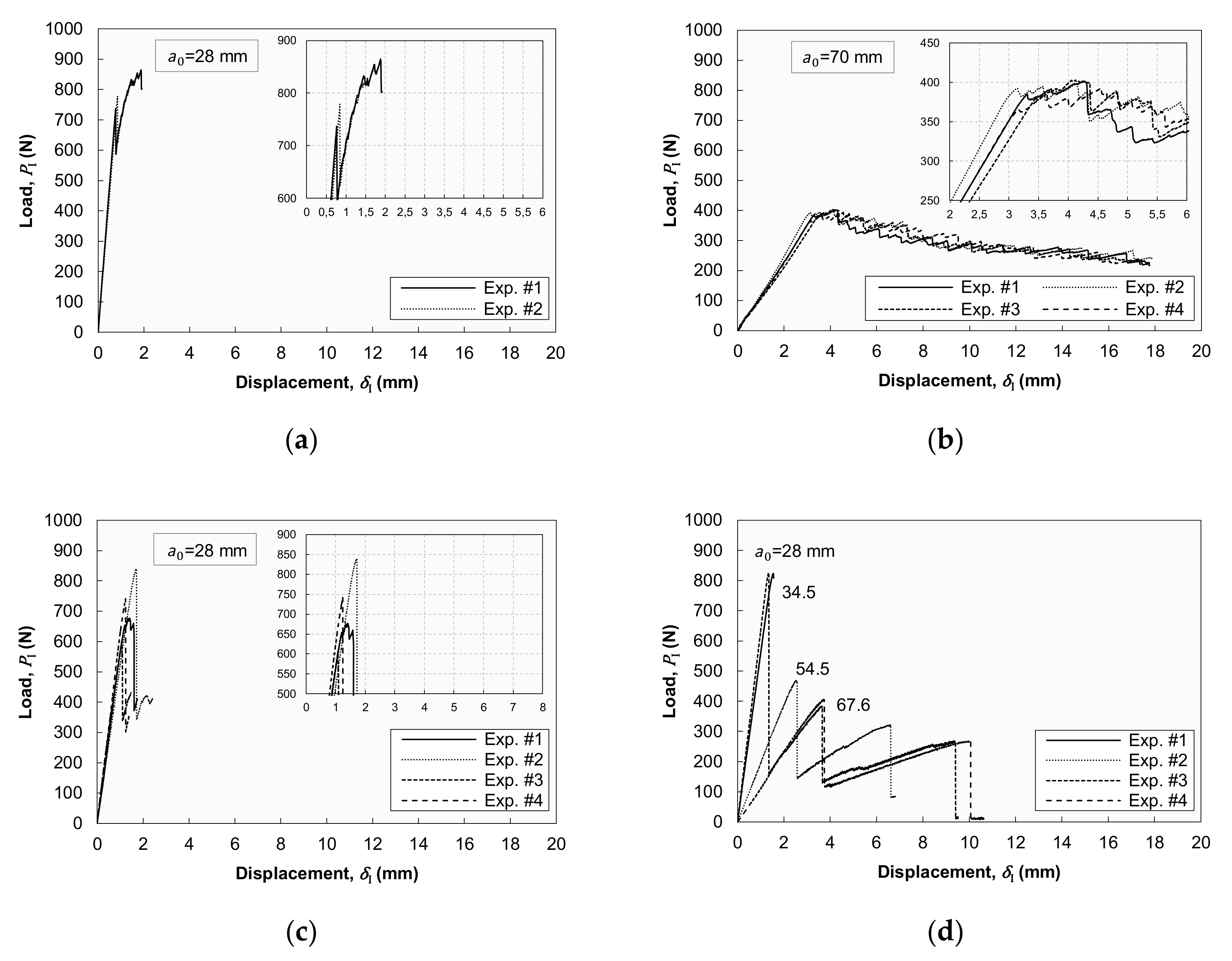
Figure 6 presents the load–displacement curves from the DCB tests. Each curve describes a successful test.
For the MO 1 specimens (Figure 6a), almost linear load–displacement behavior is observed up to the maximum load, followed by the first load drop. After this drop, the load starts increasing again in a strongly non-linear mode until it increases by almost 200 N, at which point an abrupt load drop occurs.
In MO 2 (Figure 6b), the initial portion of the curves can be characterized as approximately linear and, after reaching a maximum load of about 400 N, the load starts to decrease as the delamination propagates. The slight deviation in the slopes of the linear portions of the curves of the four specimens tested (something not observed in the previous two sets of curves) originated from the slightly different values of the initial crack length (see Section 2.5.1). During the crack propagation phase, the curves exhibit a slightly saw-toothed pattern, suggesting brittle failure.
As shown in Figure 6c, the specimens following MO 3 initially presented linear load–displacement behavior, followed by a visual deviation from linearity that occurred approximately 200 N before reaching the maximum test load. After this load, a sudden load drop associated with the abrupt propagation of the crack occurred for all four specimens tested (see Section 3.1.2).
As already mentioned, each MO 4 specimen had a different initial crack length and, as a result, each curve features a linear portion of a different slope, as well as a different maximum load. As shown in Figure 6d, with an increase in the specimen’s initial crack length, both the slope of the linear portion of the curve and the maximum load decrease. All MO 4 specimens exhibited unstable crack growth characterized by sudden load drops. The intense stick–slip behavior observed (a common phenomenon in fracture tests) was characterized by regions of almost no crack growth as the load increased and, after reaching a critical value of SERR, unstable/fast propagation of disbonding and an unexpected load drop.
Comparing the propagation phases of the four sets of curves, the MO 2 specimens are the only ones that were not very brittle, whereas the other three sets of curves present clearly brittle crack propagation behaviors characterized by almost linear load jumps. The experimental scatter for the MO 1 and 2 curves is small in both the initiation and propagation phases of the curves, while in the MO 3 curves, the scatter of the is larger.
Evidently, the load–displacement curves of the four MOs (Figure 6) cannot be directly compared since the initial crack length may significantly vary.
3.1.2. Fracture Behaviors During Testing and Fractographic Analyses
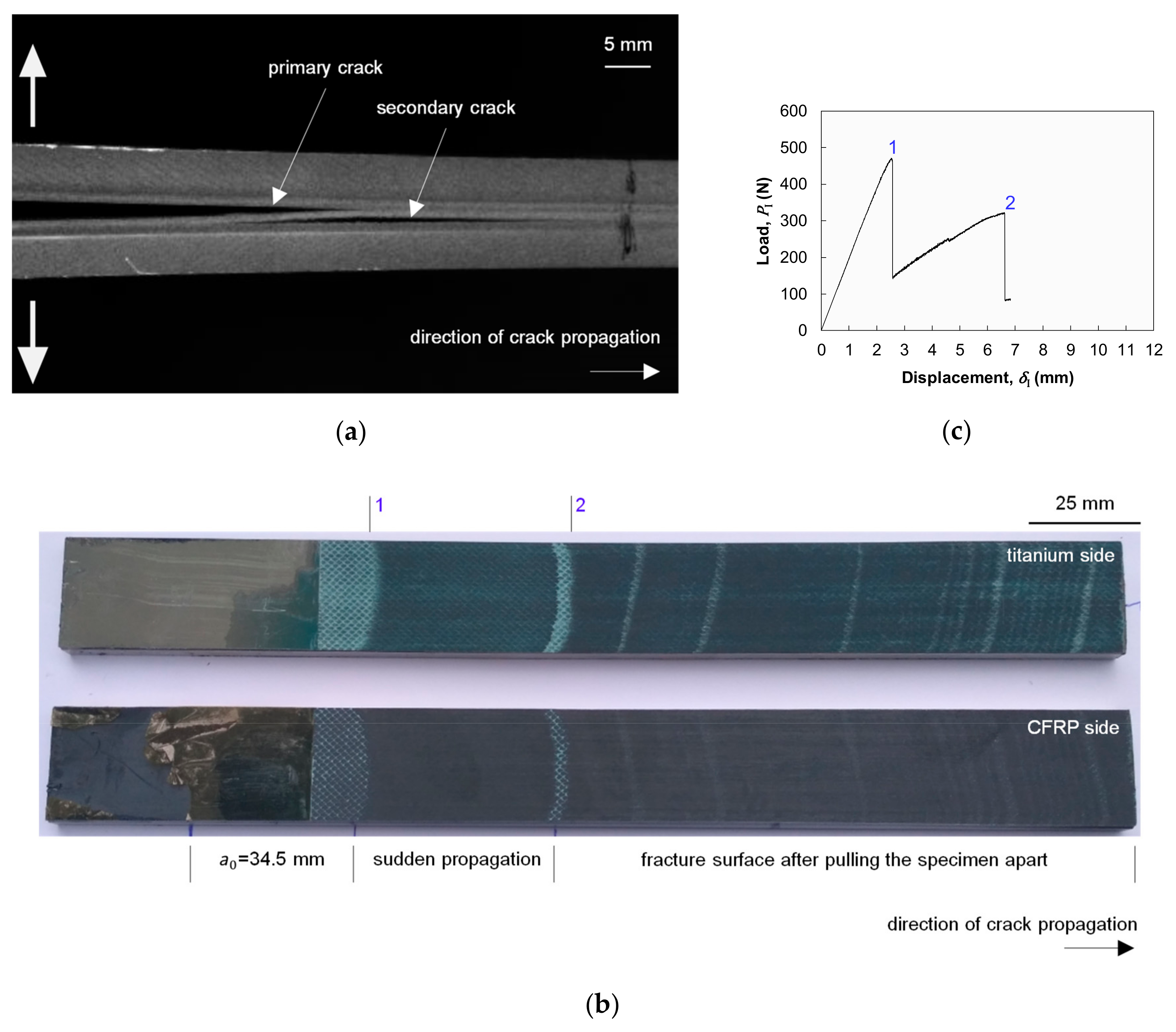
Monitoring of the crack propagation via a high-resolution camera (Figure 7a) revealed the development of adherent failure at the propagation phase of the MO 1, 2, and 3 specimens. In particular, just after initiation of the primary crack (i.e., interfacial disbonding of the adhesive layer), a secondary crack (interlaminar crack) began. The secondary crack continued to propagate simultaneously with the primary crack over the entire test. Focusing on this behavior, we deduced that the applied pre-treatment [21] created a strong titanium/CFRP interface and, consecutively, the CFRP itself became the “weak link” of the joint. Secondary cracking phenomena were also noted in [12], where, to avoid large deformations and/or adherent damage, backing beams were as well used.
MO 4 is the only MO under which no secondary cracking was observed, possibly due to the different composite (thermoplastic) material used. Figure 7b shows a photograph of the fracture surfaces of a representative MO 4 specimen and Figure 7c associates this photograph with the respective load–displacement curve presented previously. The regions of the fracture surfaces associated with the crack arrest phases of the test clearly appear rougher, likely due to the severe local plastic deformation of the adhesive layer. Contrariwise, the regions that experienced rapid propagation were smooth. We suggest that, after unstable disbonding growth, a plastically deformed region was formed in the vicinity of the crack tip, thereby explaining the stick–slip behavior of the specimens. As long as the crack remained arrested inside this region, it propagated slowly. Observing the fracture surfaces of Figure 7b, the stable crack propagation regions appear a lighter color (light-gray) than the unstable ones (dark-grey color).
The failure mode percentages of the four MOs, classified as in Section 2.6, are presented in Table 3. For MOs 1, 2, and 3, due to the presence of adherent failure (a secondary crack), it was unnecessary to examine the fracture surfaces and extract the failure mode percentages. Conversely, for MO 4, a combination of adhesive, cohesive, and thin-layer cohesive failure modes is observed. Between them, the first failure mode is dominant, meaning that the adhesive is not fully exploited in this MO.
3.1.3. Fracture Toughness Performance
Utilizing the load–displacement data presented in Section 3.1.1, we next calculate the total SERR and mode mixity of the joint under consideration. The calculation results are summarized in Table 4, where the crack initiation loads, initial crack lengths, and initiation fracture toughness (expressed by the magnitudes SERR and mode mixity) are presented for the four MOs. As shown in this table, MO 4 provides the highest average SERR value, while the worst ones are provided by MOs 1 and 3. At the crack initiation load, the mode mixity remains quite low for all MOs, meaning that the prevailing loading conditions at the crack tip can be considered (nearby) pure mode I conditions.
3.2. Results from the End-Notched Flexure (ENF) Experiments
3.2.1. Load–Displacement Curves
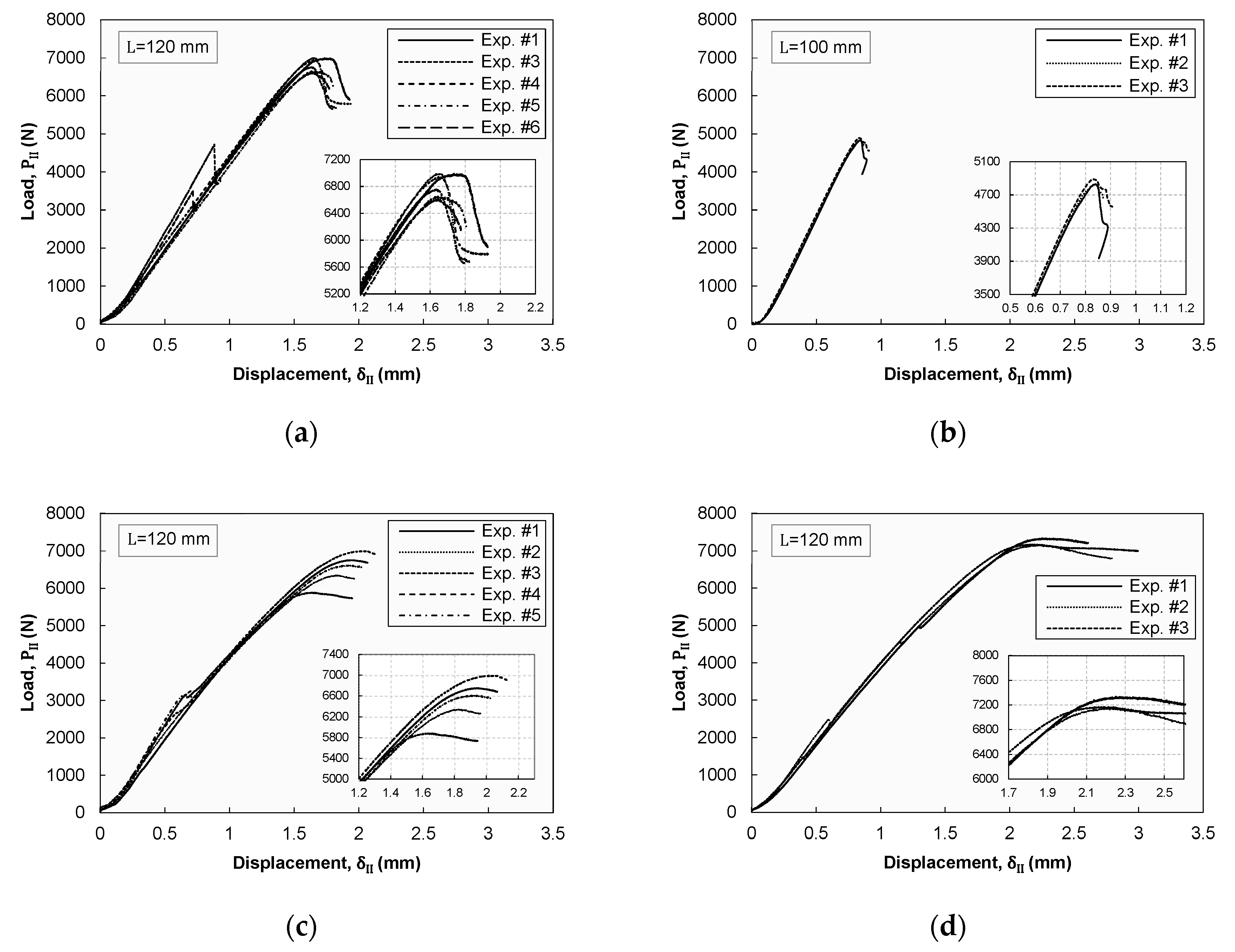
Figure 8 presents the load versus displacement curves from the ENF experiments of all MOs. Every curve corresponds to one successful experiment, while the four different diagrams serve to compare the fracture behaviors of the four different MOs studied.
In general, all curves can be understood as a sequence of three distinct phases. In the first phase, the slope of the curve, and thus the material behavior, is linear. In the second phase, we observe a loss of linearity, which typically suggests the appearance of some irreversible fracture processes, such as plastic deformation or damage formation inside the interface layer. Last, in the third phase, a major load drop is noted that corresponds to the propagation of the disbonding crack.
In the curves of all MOs, and especially in those of MOs 1, 2, and 4, the load drop is relatively “smooth”, implying a gradual degradation of material properties. In the second phase, matrix micro-cracking phenomena are likely present, but not titanium/aluminum yielding or fiber rupture phenomena, as ensured by the design of the specimens [19]. For MOs 1, 3, and 4, the slight load drops observed in the respective plots of Figure 8 are associated with the failure of excess adhesive located on the starter crack area. As demonstrated by the curves, these load drops did not affect the subsequent fracture response of the specimens.
As already commented, the span length of the MO 2 ENF specimens was shorter than that of the MO 1, 2, and 3 specimens, so the load–displacement curves of that MO, as shown in Figure 8b, are not directly comparable to those of the other MOs. Nevertheless, the SERR values of the four MOs (to be presented in Section 3.2.3) are obviously comparable to each other.
3.2.2. Fracture Behaviors During Testing and Fractographic Analyses
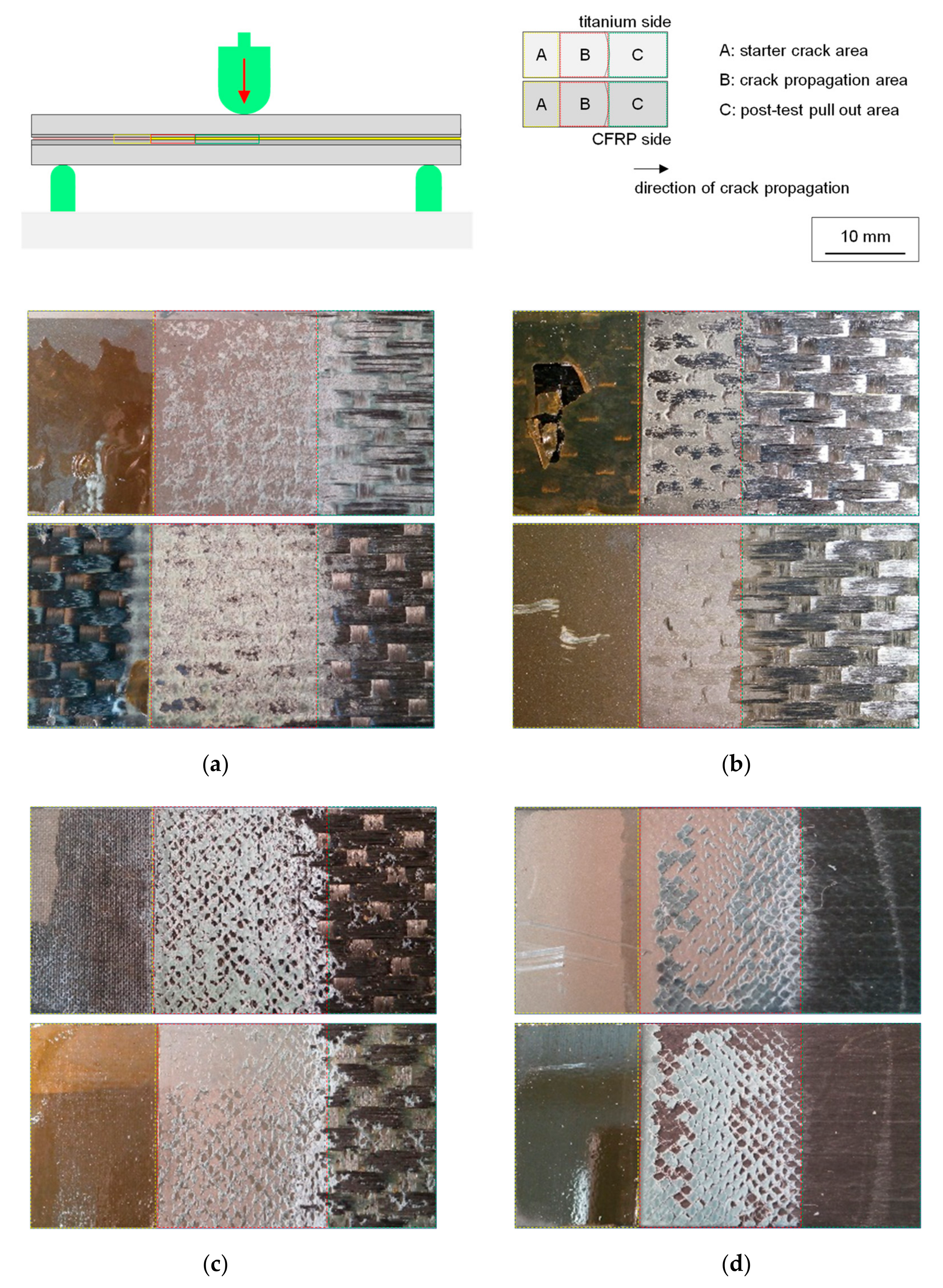
Representative macro-photographs of the fracture surfaces of the ENF specimens are presented in Figure 9. The titanium and CFRP sides’ fracture surfaces are arranged side by side, with the first to appear at the top of each sub-figure and the second at the bottom. The position of the starter crack, the crack propagation area, and the post-test pull out area are in all photographs marked by dotted frames of different colors. The direction of the crack propagation extends from left to right.
As shown in Figure 9, the failure surfaces of the MO 3 and 4 specimens are strongly affected by the presence of a knit carrier. In these MOs, the carrier (or the imprints left by the carrier’s bundles of fibers) can be clearly seen on the fracture surfaces, forming a characteristic rhombic pattern. Furthermore, someone may imply that the nodes of the carrier may contribute to the enhancement of the fracture toughness of the joint. Conversely, for MO 1, the mat carrier is not clearly shown. The different composite substrates between MOs 1–3 and 4 are clearly shown in Figure 9.
In Table 5, the failure mode percentages of the four MOs are tabulated. For all MOs, a combination of the four different failure modes (“adhesive”, “thin cohesive, titanium”, “thin cohesive, CFRP”, and “cohesive”) was observed. Among them, the “thin cohesive, titanium” mode was the dominant failure mode for MOs 1, 3, and 4. For MO 2, which is the only non-adhesive MO, cohesive failure is the dominant failure mode. In principle, the desired failure mode is cohesive failure because it implies that the qualities of both the adhesive and bonding process are optimal.
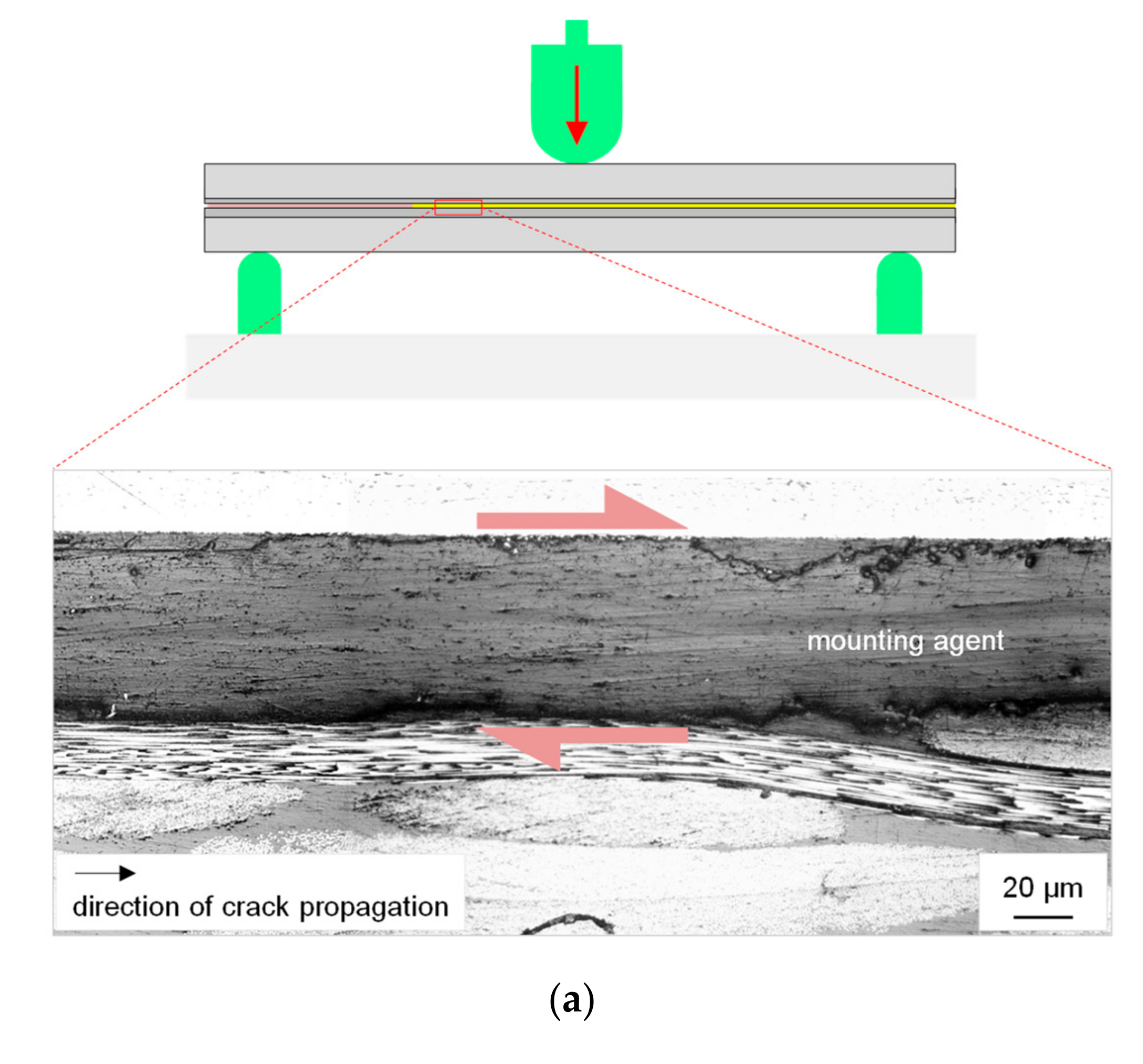
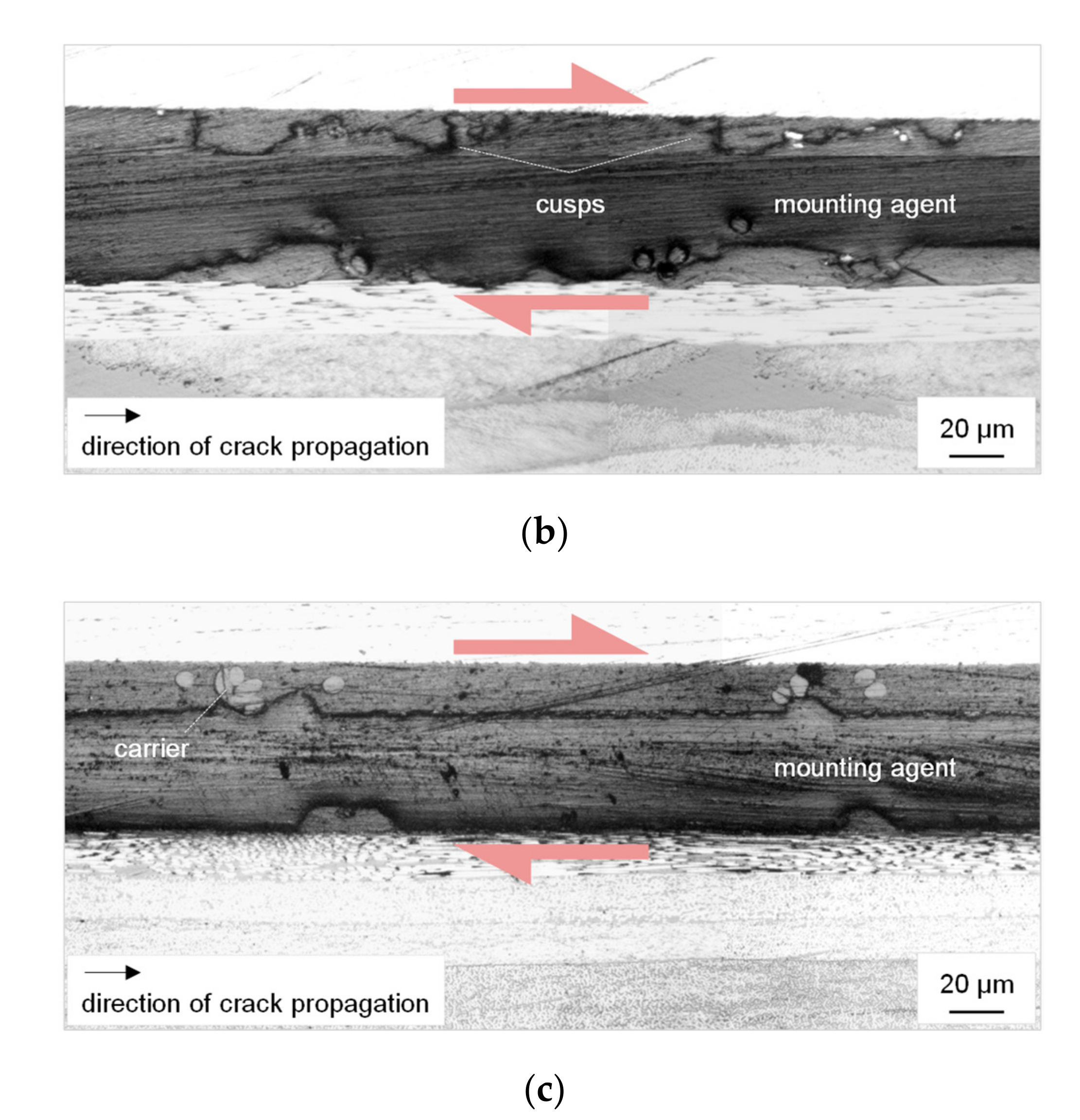
Figure 10 shows representative fractographic images of the longitudinal views of the specimens. The sketch of this figure shows the region of interest. In Figure 10a–c, the titanium substrate can be seen at the top, while some of the CFRP layers are observable at the bottom. The mounting agent that the sample was embedded into during the sample preparation process is visible in the central regions of each image. The regions corresponding to adhesive or thin/thick cohesive failure are likewise shown just above and below this agent.
As evident in Figure 10, the crack path for each MO was different. In MOs 1 and 3, the crack path switched between two different planes—i.e., between the adhesive/titanium and adhesive/CFRP planes, a process that increased the percentage of the cohesive failure and, consequently, enhanced the fracture toughness of the joint. Conversely, in MO 4, the fracture occurred only along the adhesive/CFRP interface plane.
Due to the three-point bending applied to the specimen, the two sub-laminates were forced to move in opposite directions relative to one another (the pink arrows in the figure show these directions). At the same time, the interface layer was loaded in shear. As a consequence, irregular cusps were formed, especially for MOs 3 and 4. In both cases, the cusps were larger and more pronounced, possibly due to the larger thickness of the applied adhesive. The creation of these cusps was largely due to the presence of the bundles of the knit carrier, as also suggested by Figure 9c,d.
3.2.3. Fracture Toughness Performance
Unlike the curves from the DCB tests, the ENF curves (Figure 8) cannot provide a good indication of the crack initiation point. Nevertheless, following the method presented in Section 2.7.1, we were able to estimate the initiation point, and the resulting values are shown in Table 6.
Next, to quantitatively compare the four MOs, the total SERRs and mode mixities for all MOs were calculated for and are presented in Table 6. The calculation results show that the highest SERR performance was achieved by MO 4, while the worst-performing MO was MO 2. For , the mode mixity was practically negligible (lower than 1%) for all MOs.
4. Conclusions
The present paper presented the results of an experimental investigation on the mode I and II interfacial fracture toughness of a titanium–CFRP adhesive joint. The intended industrial application of this joint requires that both the titanium and CFRP adherents be very thin (thinner than 1.5 mm). To be able to perform valid experiments on this thin joint while avoiding large/plastic deformation phenomena that would make our post-testing fracture toughness calculations invalid, we first stiffened it by bonding the aluminum backing beams.
The manufacturing of the joint was realized by following four MOs that are cost-effective and typically adopted by the industry. These options use either co-bonding or secondary bonding techniques, as well as different composite materials, adhesive agents, and/or curing temperatures. The characterization program included mechanical experiments (using the DCB and ENF configurations), as well as fractographic investigations. Subsequently, the four MOs were compared in terms of their fracture toughness by calculating the SERR. To determine the SERR, we utilized an analytical model that was published by the first two authors in [2].
The main conclusions of the present work can be summarized as follows:
For the DCB experiments:
- Concerning MOs 1, 2, and 3, the interface between titanium and CFRP proved to be tough after the performed surface pre-treatment. Thus, the “weak link” of the joint was transferred to the interface between the first and second composite layer. As a result, during the DCB test, delaminations were formed and propagated through this interface. On the contrary, no adherent failure was observed in the MO 4 specimens, while the principal failure mode was adhesive failure.
- In terms of initiation fracture toughness, calculated as the total SERR at , the best and worst performing MOs were MOs 4 and 1, respectively. According to the utilized data reduction model, they attained SERR values equal to 874 N/m (MO 4) and 467 N/m (MO 1).
- Due to the bending–extension coupling and residual thermal stresses effects, mode mixity was inevitably introduced in all tests. The mode mixity was, however, consistently low at (lower that 6.1%) for all MOs.
Regarding the ENF experiments:
- The three failure modes observed in the ENF tests were adhesive failure, cohesive failure, and thin-layer cohesive failure. Between them, the primary failure mode for all MOs was the third one. No secondary cracking/adherent failure phenomena were observed.
- In terms of initiation fracture toughness, calculated as the total SERR at , the best and worst performing MOs were MOs 4 and 2, respectively. According to the utilized data reduction scheme, MO 4 attained a SERR value of 2820 N/m, while the corresponding value for MO 2 was 1296 N/m.
- The “parasitic” mode mixity during the ENF experiments was practically negligible at since its value was lower than 1% for all MOs.
To the best of our knowledge, this paper is the first to report experimental results on the interfacial fracture toughness of multi-layered metal–composite joints with bending–extension coupling and residual thermal stresses effects, as well as manufactured following different characteristic industry relevant approaches. We hope that the work’s findings will be, in the future, interesting for many applications that involve hybrid metal–composite joining in several industrial fields.
Although beyond the scope of this paper, a detailed exploration of the involved failure mechanisms in the micro-scale using scanning electron microscopy (SEM) may be an interesting future extension of our research.
Author Contributions
Conceptualization, P.T. and T.L.; methodology, P.T. and T.L.; software, P.T.; validation, P.T.; formal analysis, P.T.; investigation, P.T. and P.N.; resources, P.N.; data curation, P.T.; writing—original draft preparation, P.T.; writing—review and editing, P.T. and T.L.; visualization, P.T.; supervision, T.L.; project administration, T.L.; funding acquisition, T.L. All authors have read and agreed to the published version of the manuscript.
Funding
This research was funded by the Clean Sky 2 Joint Undertaking under the European Union’s Horizon 2020 program TICOAJO, grant number 737785.
Acknowledgments
The authors thank their TICOAJO partners from the Royal Netherlands Aerospace Centre (NLR), The Netherlands, and especially Wouter M. van den Brink, for assisting with the manufacturing of the test specimens and part of the experiments. The authors thank their colleagues from the Laboratory of Applied Mechanics and Vibrations, University of Patras, Greece, and especially Dimitrios Pegkos and George Sotiriadis, for assisting with the execution of most of the experiments. The authors thank their TICOAJO partners from the Structural Integrity and Composites (SI&C) research group, Delft University of Technology, the Netherlands, and especially Wandong Wang, Johannes A. Poulis, Sofia Teixeira de Freitas, and Dimitrios Zarouchas, for performing the surface pre-treatment studies.
Conflicts of Interest
The authors declare no conflict of interest.
References
- Yokozeki, T. Energy release rates of bi-material interface crack including residual thermal stresses: Application of crack tip element method. Eng. Fract. Mech. 2010, 77, 84–93. [Google Scholar] [CrossRef]
- Tsokanas, P.; Loutas, T. Hygrothermal effect on the strain energy release rates and mode mixity of asymmetric delaminations in generally layered beams. Eng. Fract. Mech. 2019, 214, 390–409. [Google Scholar] [CrossRef]
- Soboyejo, W.O.; Lu, G.-Y.; Chengalva, S.; Zhang, J.; Kenner, V. A modified mixed-mode bending specimen for the interfacial fracture testing of dissimilar materials. Fatigue Fract. Eng. Mater. Struct. 1999, 22, 799–810. [Google Scholar] [CrossRef]
- Ouyang, Z.; Ji, G.; Li, G. On approximately realizing and characterizing pure mode-I interface fracture between bonded dissimilar materials. J. Appl. Mech. 2011, 78, 031020. [Google Scholar] [CrossRef]
- Khoshravan, M.; Mehrabadi, F.A. Fracture analysis in adhesive composite material/aluminum joints under mode-I loading; experimental and numerical approaches. Int. J. Adhes. Adhes. 2012, 39, 8–14. [Google Scholar] [CrossRef]
- Alía, C.; Arenas, J.M.; Suárez, J.C.; Ocaña, R.; Narbón, J.J. Mode II fracture energy in the adhesive bonding of dissimilar substrates: Carbon fibre composite to aluminium joints. J. Adhes. Sci. Technol. 2013, 27, 2480–2494. [Google Scholar] [CrossRef] [Green Version]
- Reeder, J.R.; Demarco, K.; Whitley, K.S. The use of doubler reinforcement in delamination toughness testing. Compos. Part A Appl. Sci. Manuf. 2004, 35, 1337–1344. [Google Scholar] [CrossRef]
- Davidson, P.; Waas, A.M.; Yerramalli, C.S. Experimental determination of validated, critical interfacial modes I and II energy release rates in a composite sandwich panel. Compos. Struct. 2012, 94, 477–483. [Google Scholar] [CrossRef]
- Ševčík, M.; Shahverdi, M.; Hutař, P.; Vassilopoulos, A.P. Analytical modeling of mixed-mode bending behavior of asymmetric adhesively bonded pultruded GFRP joints. Eng. Fract. Mech. 2015, 147, 228–242. [Google Scholar] [CrossRef]
- Bienias, J.; Dadej, K.; Surowska, B. Interlaminar fracture toughness of glass and carbon reinforced multidirectional fiber metal laminates. Eng. Fract. Mech. 2017, 175, 127–145. [Google Scholar] [CrossRef]
- Zakaria, A.Z.; Shelesh-nezhad, K.; Chakherlou, T.N.; Olad, A. Effects of aluminum surface treatments on the interfacial fracture toughness of carbon-fiber aluminum laminates. Eng. Fract. Mech. 2017, 172, 139–151. [Google Scholar] [CrossRef]
- Manikandan, P.; Chai, G.B. Mode-I metal-composite interface fracture testing for fibre metal laminates. Adv. Mater. Sci. Eng. 2018, 4572989. [Google Scholar] [CrossRef] [Green Version]
- Zambelis, G.; da Silva Botelho, T.; Klinkova, O.; Tawfiq, I.; Lanouette, C. Evaluation of the energy release rate in mode I of asymmetrical bonded composite/metal assembly. Eng. Fract. Mech. 2018, 190, 175–185. [Google Scholar] [CrossRef]
- Hua, X.; Li, H.; Lu, Y.; Chen, Y.; Qiu, L.; Tao, J. Interlaminar fracture toughness of GLARE laminates based on asymmetric double cantilever beam (ADCB). Compos. Part B Eng. 2019, 163, 175–184. [Google Scholar] [CrossRef]
- Wang, J.; Qiao, P. On the energy release rate and mode mix of delaminated shear deformable composite plates. Int. J. Solids Struct. 2004, 41, 2757–2779. [Google Scholar] [CrossRef]
- Mohan, J.; Ivanković, A.; Murphy, N. Mixed-mode fracture toughness of co-cured and secondary bonded composite joints. Eng. Fract. Mech. 2015, 134, 148–167. [Google Scholar] [CrossRef]
- González Ramírez, F.M.; Garpelli, F.P.; de Cássia Mendonça Sales, R.; Cândido, G.M.; Arbelo, M.A.; Shiino, M.Y.; Donadon, M.V. Experimental characterization of mode I fatigue delamination growth onset in composite joints: A comparative study. Mater. Design 2018, 160, 906–914. [Google Scholar] [CrossRef]
- van den Brink, W.M.; Tsokanas, P.; Nijhuis, P.; Loutas, T. Moment Loading Testing and Data Reduction for Characterizing the Fracture Toughness of Hybrid Joints. In Proceedings of the 7th ECCOMAS Thematic Conference on the Mechanical Response of Composites, Girona, Spain, 18–20 September 2019. [Google Scholar]
- Tsokanas, P.; Loutas, T.; Kotsinis, G.; Kostopoulos, V.; van den Brink, W.M.; de la Escalera, F.M. On the fracture toughness of metal-composite adhesive joints with bending-extension coupling and residual thermal stresses. Compos. Part B Eng. 2020, 185, 107694. [Google Scholar] [CrossRef]
- Adamos, L.; Tsokanas, P.; Loutas, T. An experimental study of the interfacial fracture behavior of Titanium/CFRP adhesive joints under mode I and mode II fatigue. Int. J. Fatigue 2020, 136, 105586. [Google Scholar] [CrossRef]
- Loutas, T.; Tsokanas, P.; Kostopoulos, V.; Nijhuis, P.; van den Brink, W.M. Mode I fracture toughness of asymmetric metal-composite adhesive joints. Mater. Today Proc. 2020. [Google Scholar] [CrossRef] [Green Version]
- Tsokanas, P.; Loutas, T.; Pegkos, D.; Sotiriadis, G.; Kostopoulos, V. Mode II fracture toughness of asymmetric metal-composite adhesive joints. MATEC Web Conf. 2019, 204, 01004. [Google Scholar] [CrossRef]
Figure 1.
Schematic of the titanium–CFRP adhesive joint under study. (a) The primary joint between the titanium and CFRP is stiffened by two aluminum beams (sketch presented in scale), reproduced from [19], with permission from Elsevier, 2020. (b) A schematic presentation of the four manufacturing options (MOs) under consideration: (i) MO 1, (ii) MO 2, (iii) MO 3, and (iv) MO 4.

Figure 2.
Photographs of the produced titanium–CFRP adhesive joint (reproduced from [19], with permission from Elsevier, 2020). (a) All produced panels showed intense curvature as a result of the manufacturing-induced residual thermal stresses. (b) The specimens cut from the panels also show an intense curvature along their length.

Figure 3.
A schematic representation (in scale) of the experimental setup and a typical photograph during the experiment for the double cantilever beam (DCB) (a) and the end-notched flexure (ENF) (b) experiments (photographs are reproduced from [19], with permission from Elsevier, 2020).
Figure 3.
A schematic representation (in scale) of the experimental setup and a typical photograph during the experiment for the double cantilever beam (DCB) (a) and the end-notched flexure (ENF) (b) experiments (photographs are reproduced from [19], with permission from Elsevier, 2020).

Figure 4.
(a) Classification of the failure modes of interest in the present study (the sketches are not in scale): (i) FM1, adhesive failure; (ii) FM2, cohesive failure; (iii) FM3, thin-layer cohesive failure, titanium side; (iv) FM4, thin-layer cohesive failure, CFRP side; and (v) FM5, adherent failure. (b) The method followed to deduce the fracture mode percentages. (i) Photograph of the fracture surface under examination. (ii) Processing the photograph using the ImageJ software. (iii) Color scale-based determination of the failure mode percentage.

Figure 5.
(a) An example load–displacement curve from a double cantilever beam (DCB)/end-notched flexure (ENF) test and determination of the crack initiation load following the three criteria defined in the ASTM D5528 standard. (b) Schematic representation of the beam model [2] utilized for experimental data reduction. We use a cantilever beam consisting of an elastic and laminated material that, due to the presence of an asymmetric through-the-width crack (i.e., delamination or interfacial disbonding), is split into two sub-laminates with thicknesses h1 and and arbitrary stacking sequences. The beam is loaded at its left end by concentrated and vertical loads (i.e., the loads , , and , where is the contact force between the upper and lower unbonded arms of the beam). The beam is also stressed by residual hygrothermal stresses. , , and are the beam’s width (not shown in the figure), total length, and initial crack length, respectively. and are the crack-tip forces, and , , and , = 1, 2, are the internal forces and moments developed at various cross-sections of the beam.

Figure 6.
Load () versus crack opening displacement () curves from the double cantilever beam (DCB) experiments for the four manufacturing options (MOs) under study: (a) MO 1, (b) MO 2, (c) MO 3, and (d) MO 4. is the initial crack length.
Figure 6.
Load () versus crack opening displacement () curves from the double cantilever beam (DCB) experiments for the four manufacturing options (MOs) under study: (a) MO 1, (b) MO 2, (c) MO 3, and (d) MO 4. is the initial crack length.

Figure 7.
(a) A representative snapshot capturing the development of a secondary crack, interlaminar between the CFRP’s first and second layers, during the experimental testing of the specimens using manufacturing option (MO) 1. The MO 2 and 3 specimens exhibited the same behavior. (b) Fracture surfaces of a typical specimen from MO 4 and (c) their correlation with the respective load–displacement curve.

Figure 8.
Load () versus crosshead displacement () curves from the end-notched flexure (ENF) experiments for the four manufacturing options (MOs) under study: (a) MO 1, (b) MO 2, (c) MO 3, and (d) MO 4. is the span length of the ENF configuration.
Figure 8.
Load () versus crosshead displacement () curves from the end-notched flexure (ENF) experiments for the four manufacturing options (MOs) under study: (a) MO 1, (b) MO 2, (c) MO 3, and (d) MO 4. is the span length of the ENF configuration.

Figure 9.
Fracture surfaces of a representative end-notched flexure (ENF) specimen from each of the four manufacturing options (MOs) studied: (a) MO 1, (b) MO 2, (c) MO 3, and (d) MO 4.
Figure 9.
Fracture surfaces of a representative end-notched flexure (ENF) specimen from each of the four manufacturing options (MOs) studied: (a) MO 1, (b) MO 2, (c) MO 3, and (d) MO 4.

Figure 10.
Microscopic images of the side-views of a representative end-notched flexure (ENF) specimen from each of the following manufacturing options (MOs): (a) MO 1, (b) MO 3, and (c) MO 4.
Figure 10.
Microscopic images of the side-views of a representative end-notched flexure (ENF) specimen from each of the following manufacturing options (MOs): (a) MO 1, (b) MO 3, and (c) MO 4.


Table 1.
Engineering constants, coefficients of thermal expansion (CTEs), and thicknesses of the materials constituting the titanium–CFRP adhesive joint.
Table 1.
Engineering constants, coefficients of thermal expansion (CTEs), and thicknesses of the materials constituting the titanium–CFRP adhesive joint.
| Material | (GPa) | (GPa) | (GPa) | (-) | Thickness (mm) | |
|---|---|---|---|---|---|---|
| Titanium | 105.0 | - | 45.0 | 0.340 | 8.6 | 0.800 |
| Thermoset CFRP 1 | 66.0 | 66.0 | 4.5 | 0.035 | 2.9 | 0.363 |
| Thermoplastic CFRP 1 | 139.0 | 10.5 | 5.2 | 0.076 | 1.0 | 0.140 |
| Aluminum | 73.1 | - | 28.0 | 0.330 | - | 5.000 |
CTE: coefficient of thermal expansion; 1 The given properties and thicknesses refer to the level of the layer.
Table 2.
Geometrical properties of the double cantilever beam (DCB) and end-notched flexure (ENF) test configurations.
Table 2.
Geometrical properties of the double cantilever beam (DCB) and end-notched flexure (ENF) test configurations.
| Test | MO | (mm) | (mm) | |||
|---|---|---|---|---|---|---|
| DCB | 1 | 25 | 200 | 28.0 2 | 5.8 | 6.5 |
| 2 | 25 | 267 1 | 70.0 2 | 5.8 | 6.5 | |
| 3 | 25 | 200 | 28.0 2 | 5.8 | 6.5 | |
| 4 | 25 | 200 | 34.5, 54.5, 28.0, and 67.6 2 | 5.8 | 6.1 | |
| ENF | 1 | 25 | 120 | 35 | 5.8 | 6.5 |
| 2 | 25 | 100 1 | 35 | 5.8 | 6.5 | |
| 3 | 25 | 120 | 35 | 5.8 | 6.5 | |
| 4 | 25 | 120 | 35 | 5.8 | 6.1 |
MO: manufacturing option; DCB: double cantilever beam; ENF: end-notched flexure; 1 MO 2 experiments were performed in a different test fixture than the MO 1, 3, and 4 experiments; 2 Section 2.5.1 explains the different values between the four MOs. For MO 4, the reported values correspond to Exp. #1, #2, #3, and #4, respectively.
Table 3.
Failure mode percentages (%) of the four manufacturing options (MOs), as resulted by the double cantilever beam (DCB) tests.
Table 3.
Failure mode percentages (%) of the four manufacturing options (MOs), as resulted by the double cantilever beam (DCB) tests.
| MO | Failure Mode 1 | ||||
|---|---|---|---|---|---|
| FM1 | FM2 | FM3 | FM4 | FM5 | |
| 1, 2, and 3 | - | - | - | - | 100.0 (±0.0) |
| 4 | 79.3 (±6.8) | 15.9 (±7.0) | 0.0 (±0.0) | 4.8 (±1.7) | 0.0 (±0.0) |
MO: manufacturing option; FM1: adhesive failure; FM2: cohesive failure; FM3: thin-layer cohesive failure, titanium side; FM4: thin-layer cohesive failure, CFRP side; FM5: adherent failure; 1 Schematics of the failure modes are shown in Figure 4a.
Table 4.
Total strain energy release rate (SERR) () and mode mixity () values of the double cantilever beam (DCB) tests for the four manufacturing options (MOs).
Table 4.
Total strain energy release rate (SERR) () and mode mixity () values of the double cantilever beam (DCB) tests for the four manufacturing options (MOs).
| MO | Load, | Initial Crack Length, | SERR, |
Mode Mixity, |
|---|---|---|---|---|
| 1 | 739 (±23) | 28.0 | 467.0 (±32.0) | 6.1 |
| 2 | 380 (±10) | 70.0 | 683.1 (±41.0) | 5.3 |
| 3 | 711 (±77) | 28.0 | 477.0 (±136.0) | 3.7 |
| 4 | - | - | 874.4 (±134.0) | 4.1 |
MO: manufacturing option; SERR: strain energy release rate.
Table 5.
Failure mode percentages (%) of the four manufacturing options (MOs) from the end-notched flexure (ENF) tests.
Table 5.
Failure mode percentages (%) of the four manufacturing options (MOs) from the end-notched flexure (ENF) tests.
| MO | Failure Mode 1 | ||||
|---|---|---|---|---|---|
| FM1 | FM2 | FM3 | FM4 | FM5 | |
| 1 | 6.8 (±2.1) | 11.5 (±3.9) | 60.8 (±1.1) | 20.9 (±2.4) | 0.0 (±0.0) |
| 2 | 21.9 (±6.0) | 64.3 (±4.6) | 4.8 (±6.8) | 8.9 (±3.5) | 0.0 (±0.0) |
| 3 | 11.8 (±5.2) | 4.8 (±2.8) | 74.5 (±1.3) | 9.0 (±3.5) | 0.0 (±0.0) |
| 4 | 12.6 (±14.0) | 11.3 (±5.3) | 73.1 (±14.0) | 3.0 (±2.8) | 0.0 (±0.0) |
MO: manufacturing option; FM1: adhesive failure; FM2: cohesive failure; FM3: thin-layer cohesive failure, titanium side; FM4: thin-layer cohesive failure, CFRP side; FM5: adherent failure; 1 Schematics of the failure modes are shown in Figure 4a.
Table 6.
Total strain energy release rate (SERR) () and mode mixity () values of the end-notched flexure (ENF) tests, for the four manufacturing options (MOs).
Table 6.
Total strain energy release rate (SERR) () and mode mixity () values of the end-notched flexure (ENF) tests, for the four manufacturing options (MOs).
| MO | Load, | SERR, | Mode Mixity, |
|---|---|---|---|
| 1 | 6550.0 (±202.5) | 2666.7 (±188.1) | 0.1 |
| 2 | 4633.3 (±102.7) | 1296.0 (±61.2) | 0.0 |
| 3 | 6002.0 (±209.8) | 2360.0 (±154.7) | 0.5 |
| 4 | 6475.0 (±309.2) | 2819.8 (±285.5) | 0.9 |
MO: manufacturing option; SERR: strain energy release rate.
© 2020 by the authors. Licensee MDPI, Basel, Switzerland. This article is an open access article distributed under the terms and conditions of the Creative Commons Attribution (CC BY) license (http://creativecommons.org/licenses/by/4.0/).
Share and Cite
MDPI and ACS Style
Tsokanas, P.; Loutas, T.; Nijhuis, P. Interfacial Fracture Toughness Assessment of a New Titanium–CFRP Adhesive Joint: An Experimental Comparative Study. Metals 2020, 10, 699. https://0-doi-org.brum.beds.ac.uk/10.3390/met10050699
AMA Style
Tsokanas P, Loutas T, Nijhuis P. Interfacial Fracture Toughness Assessment of a New Titanium–CFRP Adhesive Joint: An Experimental Comparative Study. Metals. 2020; 10(5):699. https://0-doi-org.brum.beds.ac.uk/10.3390/met10050699
Chicago/Turabian StyleTsokanas, Panayiotis, Theodoros Loutas, and Peter Nijhuis. 2020. "Interfacial Fracture Toughness Assessment of a New Titanium–CFRP Adhesive Joint: An Experimental Comparative Study" Metals 10, no. 5: 699. https://0-doi-org.brum.beds.ac.uk/10.3390/met10050699
Note that from the first issue of 2016, this journal uses article numbers instead of page numbers. See further details here.