Quality Assessment Method Based on a Spectrometer in Laser Beam Welding Process


1
Research institute, Monisys Co., Ltd., 775, Gyeongin-ro, Yeongdeungpo-Gu, Seoul 07299, Korea
2
Joining R & D Group, Korea Institute of Industrial Technology, 156 Gaetbeol-ro, Yeonsu-Gu, Incheon 21999, Korea
*
Authors to whom correspondence should be addressed.
Metals 2020, 10(6), 839; https://0-doi-org.brum.beds.ac.uk/10.3390/met10060839
Submission received: 9 June 2020
/
Revised: 23 June 2020
/
Accepted: 23 June 2020
/
Published: 24 June 2020
(This article belongs to the Special Issue Advanced Welding Technology in Metals)
Abstract
:For the automation of a laser beam welding (LBW) process, the weld quality must be monitored without destructive testing, and the quality must be assessed. A deep neural network (DNN)-based quality assessment method in spectrometry-based LBW is presented in this study. A spectrometer with a response range of 225–975 nm is designed and fabricated to measure and analyze the light reflected from the welding area in the LBW process. The weld quality is classified through welding experiments, and the spectral data are thus analyzed using the spectrometer, according to the welding conditions and weld quality classes. The measured data are converted to RGB (red, green, blue) values to obtain standardized and simplified spectral data. The weld quality prediction model is designed based on DNN, and the DNN model is trained using the experimental data. It is seen that the developed model has a weld-quality prediction accuracy of approximately 90%.
1. Introduction
The advent of Industry 4.0 has brought significant enhancements to manufacturing processes, which are now based on smart and autonomous systems, and are incorporated with data and machine learning (ML) [1]. The enhancements to smart manufacturing processes, especially concerning welding technology, must be extended and established, in the context of modern manufacturing [2]. Among various welding technologies, laser beam welding (LBW) has a higher precision, productivity, flexibility, effectiveness, and numerous other advantages, which include a deeper penetration, higher welding speed, and lower distortion, compared to other welding technologies, owing to the properties of the power sources in LBW [3,4,5,6]. In addition, the LBW is a suitable joining technology for welding dissimilar metals and advanced materials such as NiTi alloy [7,8,9]. The LBW presents a substantial potential for manufacturing applications [10], and more study on the LBW process is required to increase the benefits of the LBW. In particular, there seems to be a need of research in the field of monitoring and controlling the welding process and weld quality, which is attributed to the complexity of LBW systems and the characteristics of the LBW process. Considering that the technologies in this field are essential to develop a smart manufacturing system for LBW, extensive research must be carried out to achieve this objective.
The monitoring of a process, and consequently the quality assessment, can be divided into three categories: pre-process, in-process, and post-process [11]. The pre-process monitoring concerns the weld seam tracking before welding or ahead of the laser heat source. The in-process monitoring focuses on the monitoring of the phenomena on the welded zone during welding, such as the keyhole’s shape stability. The post-process monitoring, generally, is concerned with the weld defect detection, and the measurement of the form of the weld seam, after welding, or behind the weld pool. In the pre-process and post-process monitoring methods, ultrasonic and camera-based techniques have been dominantly used. In the case of in-process monitoring, a wider range of measuring methods, including optical (ultraviolet, visual, infrared) and acoustic detectors, X-ray radiography, and camera-based methods, have been used to adequately deal with welding phenomena generated by the high-energy-density laser.
According to Stavridis et al. [10], the in-process quality assessment, i.e., in-process monitoring of LBW, can be further sub-divided into four parts, based on the monitoring techniques used, such as image processing, acoustic emission, X-ray radiography, or optical signal techniques. Vision and thermal images are mainly used in image processing techniques to observe the weld pool [12], keyhole [13], plume, and spatters [14]. The acoustic emission techniques have been applied for the measurement of the melting, vaporization, plasma generation, keyhole formation [15], and propagation of cracks [16], and the X-ray techniques have been used to observe the welding phenomena and defects, including slag inclusions, blow holes, incomplete penetration, and undercuts [17]. In the case of optical signal techniques, they use vision systems (charge-coupled device and complementary metal–oxide–semiconductor cameras), photodiodes [18], and spectrometers (which are highly related with the topic of the study).
Sibillano et al. [19] studied the dynamics of the plasma plume, produced in LBW of 5083 aluminum alloy, with the help of correlation spectroscopy, and presented the results of the influence of welding speed on the loss of alloying elements. Rizzi et al. [20] investigated the spectroscopic signals, produced by the laser-induced plasma optical emission, together with energetic and metallographic analyses of CO2 laser-welded stainless-steel lap joint, using the response surface methodology (RSM). This statistical approach allowed the study of the influence of the laser beam power and laser welding speed, on the plasma plume electron temperature, joint penetration depth, and melted area. Konuk et al. [21] used a spectrometer to collect the optical emissions of the welding area, and calculate the electron temperature, and the data measured and calculated were used to determine the weld quality and to control the laser power. Sebestova et al. [22] designed a sensor to monitor the pulsed Nd:YAG laser welding process, based on the measurement of the plasma electron temperature, and this sensor was used to detect the weld penetration depth. Zaeh and Huber [23] investigated the radiation emission of the laser-induced plume during LBW of aluminum and steel alloys, and they developed a system to control the chemical composition of the melt pool, during the active welding process. Chen et al. [24] proposed a spectroscopic method based on a support vector machine (SVM) and artificial neural network (ANN) for the detection and classification of fiber laser welding defects. The spectral data captured by the spectrometer was processed by selecting sensitive emission lines and extracting features of the evolution of the spectral data; the SVM and ANN models were designed based on the processed spectral data. It has been verified that these two models were quite effective in detecting and classifying the weld defects. Zhang et al. [25] designed a multiple-sensor system that includes an auxiliary illumination visual sensor system, an ultraviolet- and a visible-band visual sensor system, a spectrometer, and two photodiodes to capture the real-time welding signal and determine the laser welding quality. A deep learning framework based on the stacked sparse autoencoder (SSAE) was established to model the relationship between the multi-sensor features and their corresponding welding statuses; a genetic algorithm (GA) was used to optimize the parameters of the SSAE framework. Lee et al. [26] developed an in-situ monitoring system using a spectrometer for laser welding on galvanized steel. They applied Fisher’s criterion to rank several features for extraction of the most valuable features, and then used the K-nearest neighbors and SVM algorithms to classify welding conditions related to the welding defects. Although some studies have been carried out to investigate weld quality assessment using a spectrometer in LBW process, till date, little attention has been paid to the quality assessment methodology, in LBW, based on the spectrometer and ML algorithms.
This study presents a deep neural network (DNN)-based quality assessment method in spectrometry-based LBW. We designed a spectrometer, that can measure and analyze the light reflected from the welding area in LBW process. The weld quality of LBW was classified through welding experiments, and the spectral data were analyzed using the spectrometer, according to the welding conditions and weld quality classes. Subsequently, the spectral data were converted to CIE 1931 RGB values, to standardize and simplify the spectral data. A weld quality prediction model was designed based on DNN, and the DNN model was trained using the experimental data. The weld-quality prediction accuracy of the model was calculated.
2. Experimental System and Procedure
2.1. Spectrometer Development
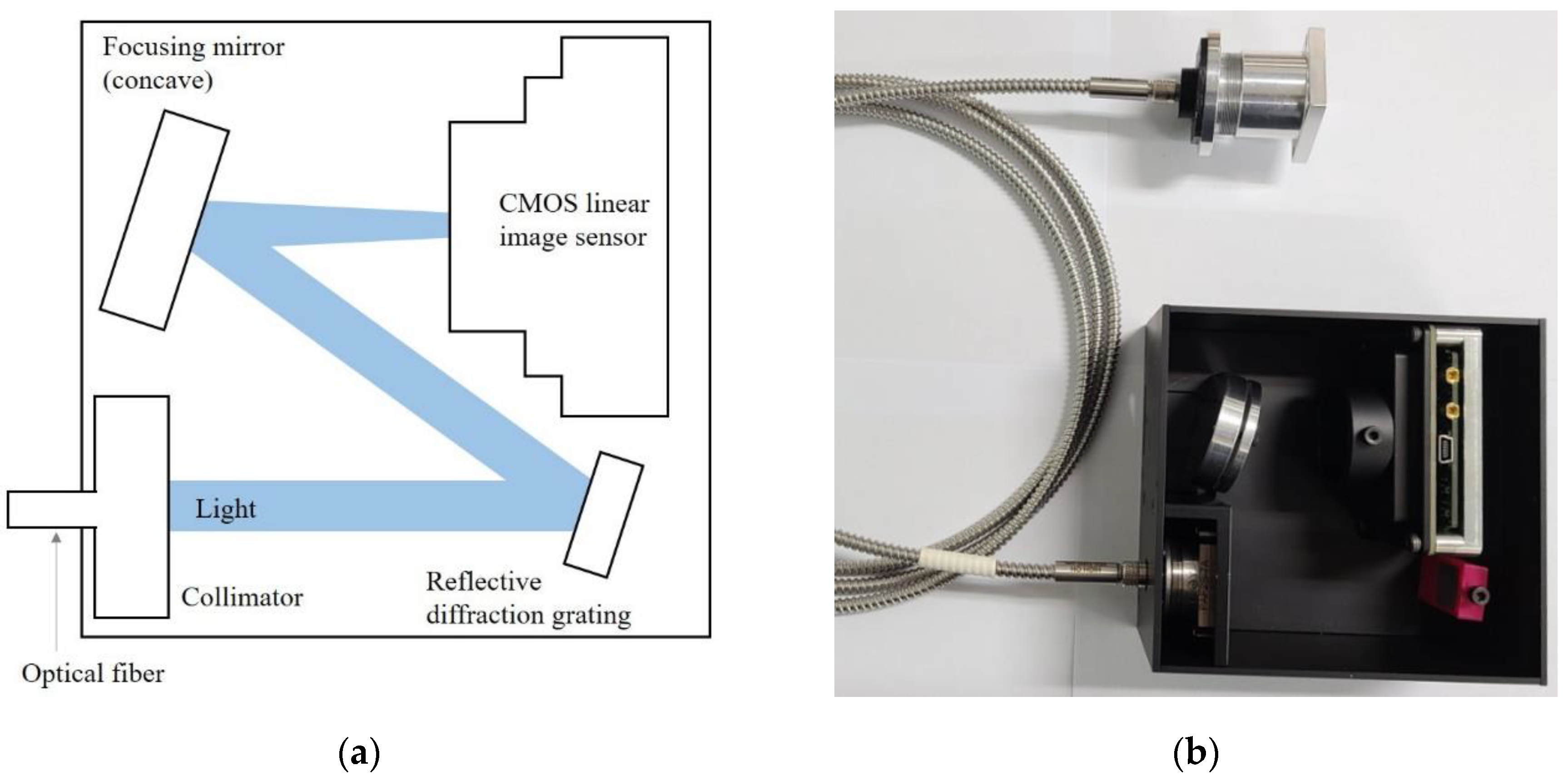
Figure 1 shows the schematic and prototype of the spectrometer designed in this study, which includes a collimator, an optical fiber, a connector, a reflective diffraction grating, a focusing mirror, and a complementary metal-oxide-semiconductor (CMOS) linear sensor. The optical fiber, through which the light enters, is connected to the collimator with an SMA (SubMiniature version A) connector. Since the round-to-linear fiber optic bundle (model No.: BFL200HS02, Thorlabs Inc., Newton, MA, USA) is used as the optical fiber, there is no need to add a separate slit as an entrance aperture. This indicates that the output terminal of the fiber optic bundle, i.e., the linear bundle, acts as the slit. The collimator (model No.: PAF2S-7A, Thorlabs Inc., Newton, MA, USA) is used to collimate the light, coming from the fiber optic bundle, and then send a collimated beam towards the grating. The reflective diffraction grating (model No.: GR13-0605, Thorlabs Inc., Newton, MA, USA) splits the photons coming from the collimator, depending on the wavelength, and then spreads the light across the focusing mirror (concave). The focusing mirror directs the light, at each wavelength, onto the CMOS linear image sensor. The line camera (model: USB line camera 8M, Coptonix GmbH, Berlin, German) which consists of a main circuit board, and the CMOS linear image sensor (model No.: S11637-1024Q, Hamamatsu, Hamamatsu City, Japan) is used as the detector. Each pixel of the CMOS linear image represents a portion of the spectrum that is translated into a measurable value, by a spectroscopy software. A dedicated software was also developed to operate the spectrometer, display the measured data, and store measurement results. The spectral response range of the developed spectrometer was 225–975 nm, and its sampling frequency was 5 kHz.
2.2. Experimental Setup and Material
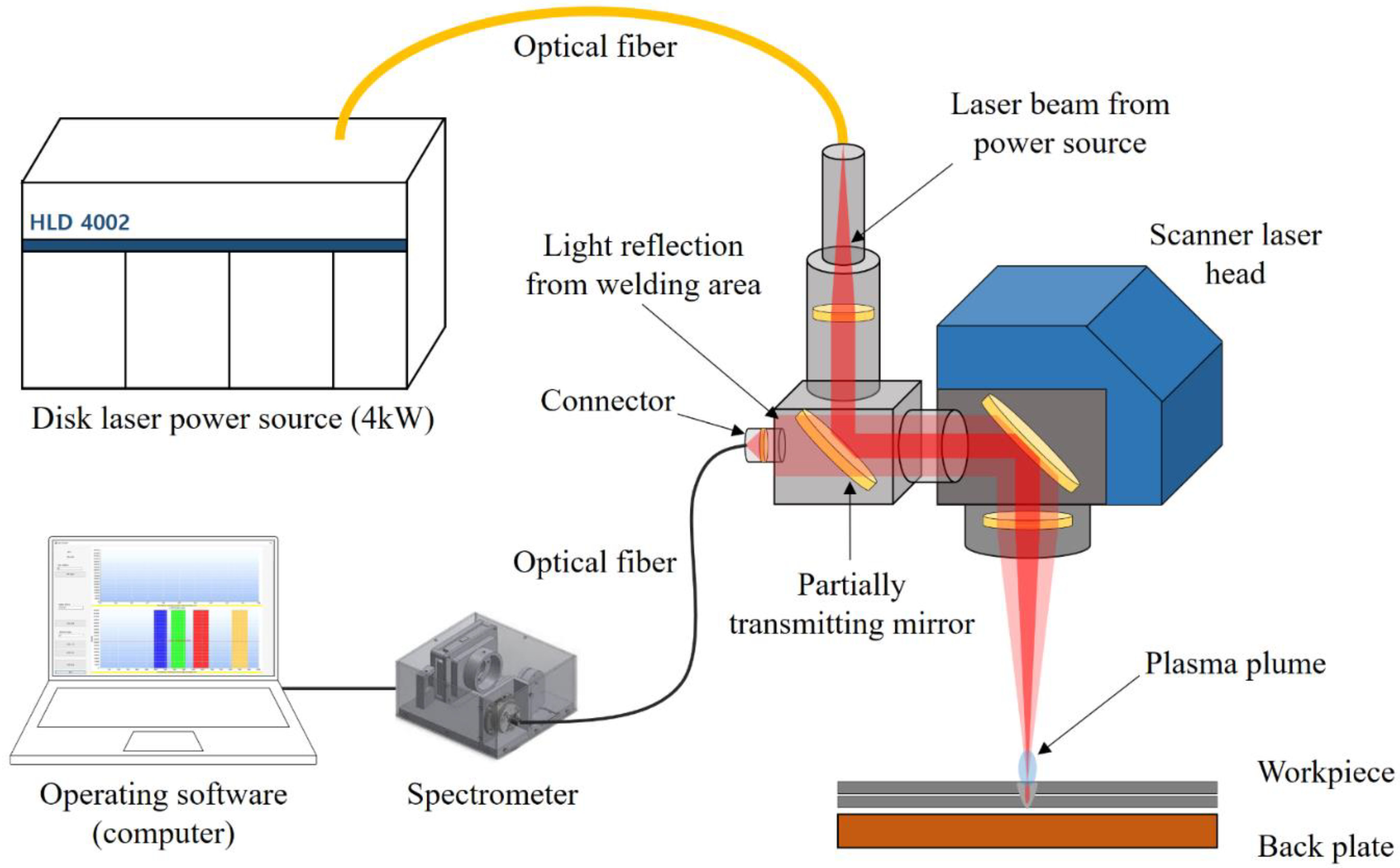
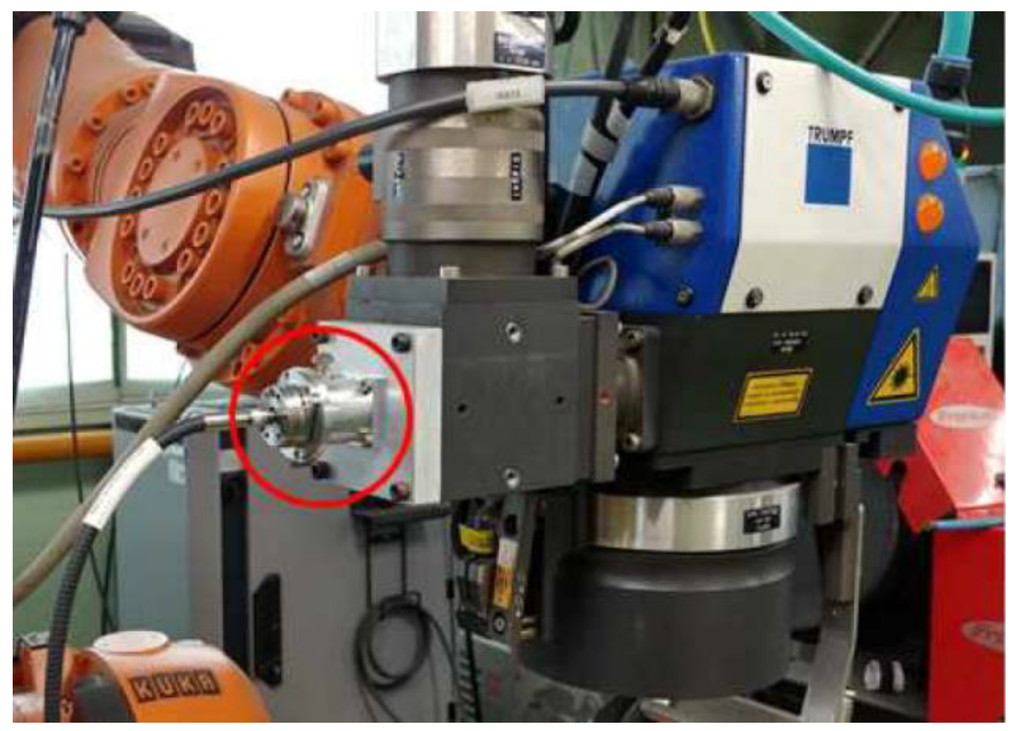
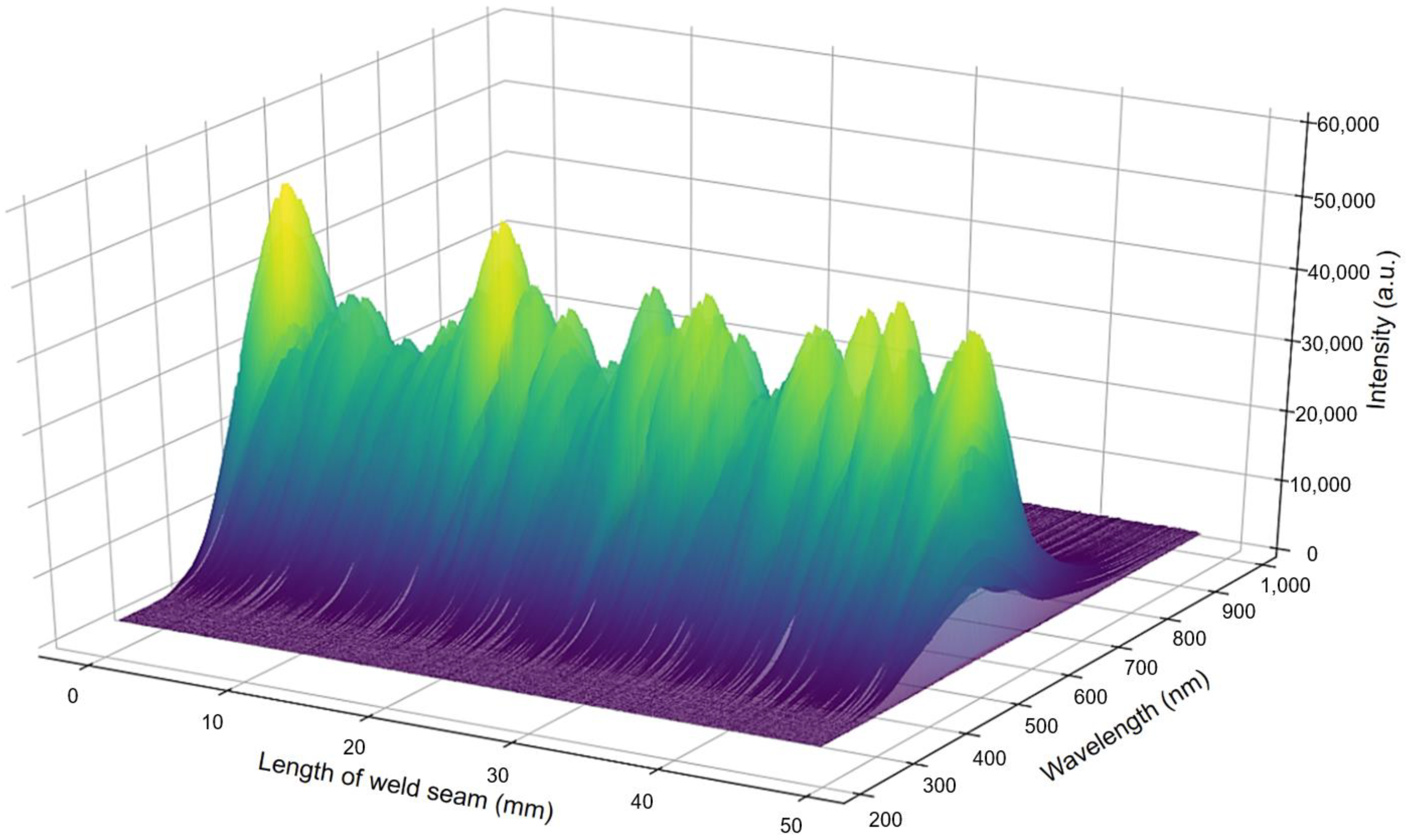
The experiment was conducted using a 4-kW disk laser welding system (model No.: TRUMPF HLD 4002, procured from Trumpf GmbH + Co. KG, Ditzingen, Germany). Figure 2 shows a diagram of the experimental setup, which was constructed by reference to the study of You and Katayama [27]. The scanner laser head was equipped with a six-axis robot arm, and was connected with two optical fibers. One of them was the round-to-linear fiber optic bundle connected to the spectrometer, and the other was the optical fiber for laser beam input transmission from the laser power source. In the former case, the scanner laser head and the fiber optic bundle were assembled with a connector, shown in Figure 3, which also has a function to condense the light entering the scanner laser head. The light emission of visible light and laser light from the welding area was transmitted to the spectrometer, through the scanner laser head (having a partially transmitting mirror) and optical fiber. The transmitted visible light emission and laser beam reflection were collimated by the collimator, and detected by the line camera. The image data obtained by the CMOS linear image sensor were sampled and digitalized at a frequency of 5 kHz. Subsequently, the processed data were collected, displayed, and stored by the computer software. Figure 4 shows a plot of the spectrum intensity variation, in LBW of lap joint configuration, with a welding speed of 1.5 m/min and a laser power of 3500 W. To test the weld quality and collect data for development of weld quality prediction models, the experiment was carried out using typical automotive high strength steel (uncoated 780 MPa-grade dual-phase (DP) steel) sheets of 1.2 mm thickness. The workpiece was cut to dimensions of 100 × 30 mm, and welding was conducted in the overlap joint configuration.
2.3. Experimental Procedure
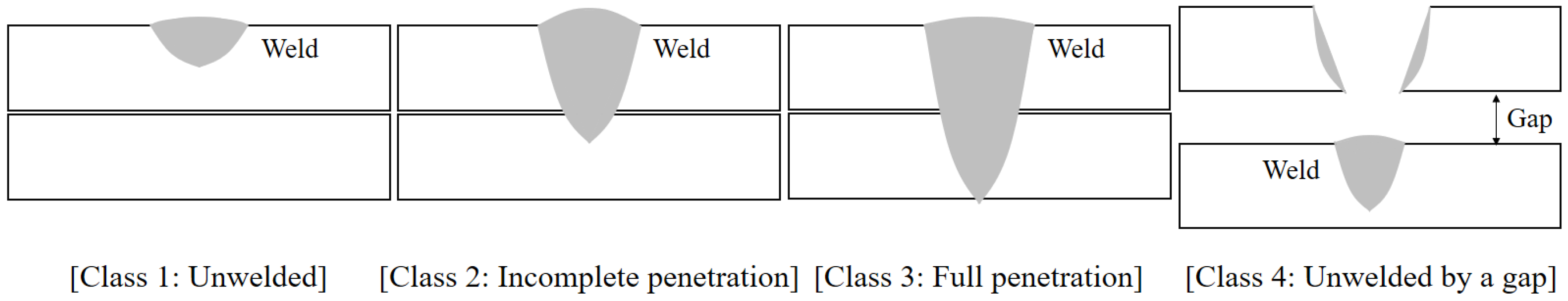
In this study, we tried to classified the weld quality into four types as shown in Figure 5:
(Class 1) Unwelded: No weld is formed between the workpieces
(Class 2) Incomplete penetration: Weld is formed between the workpieces but not full penetration
(Class 3) Full penetration: Weld fully penetrates all workpieces
(Class 4) Unwelded by a gap, between the workpieces in lap joint configuration
To evaluate the weld quality and as well as to obtain experimental data, which can be qualified according to the predefined types and are enough to develop a quality prediction model, the welding parameters were initialized with values presented in Table 1. For the laser power and the welding speed, welding was carried out twice (2 replicates) in all possible conditions (21 combinations), at a gap of 0 mm. At a gap of 0.8 mm, welding was carried out only at laser powers of 3000 and 4000 W for all welding speeds, which means that welding was performed under six conditions for two replicates. All welding runs were carried out with a length of 50 mm in the lap joint configuration. The diameter of a focused laser beam was 0.6 mm, and the wavelength of disk laser was 1030 nm. The defocused distance was fixed at 0 mm. Argon (Ar) inert gas was used as shielding gas, and the flow rate of the shield gas was set to 20 L/min. The metal back plate was set under the workpieces as shown in Figure 1.
3. Results and Discussion
3.1. Weld Quality Evaluation
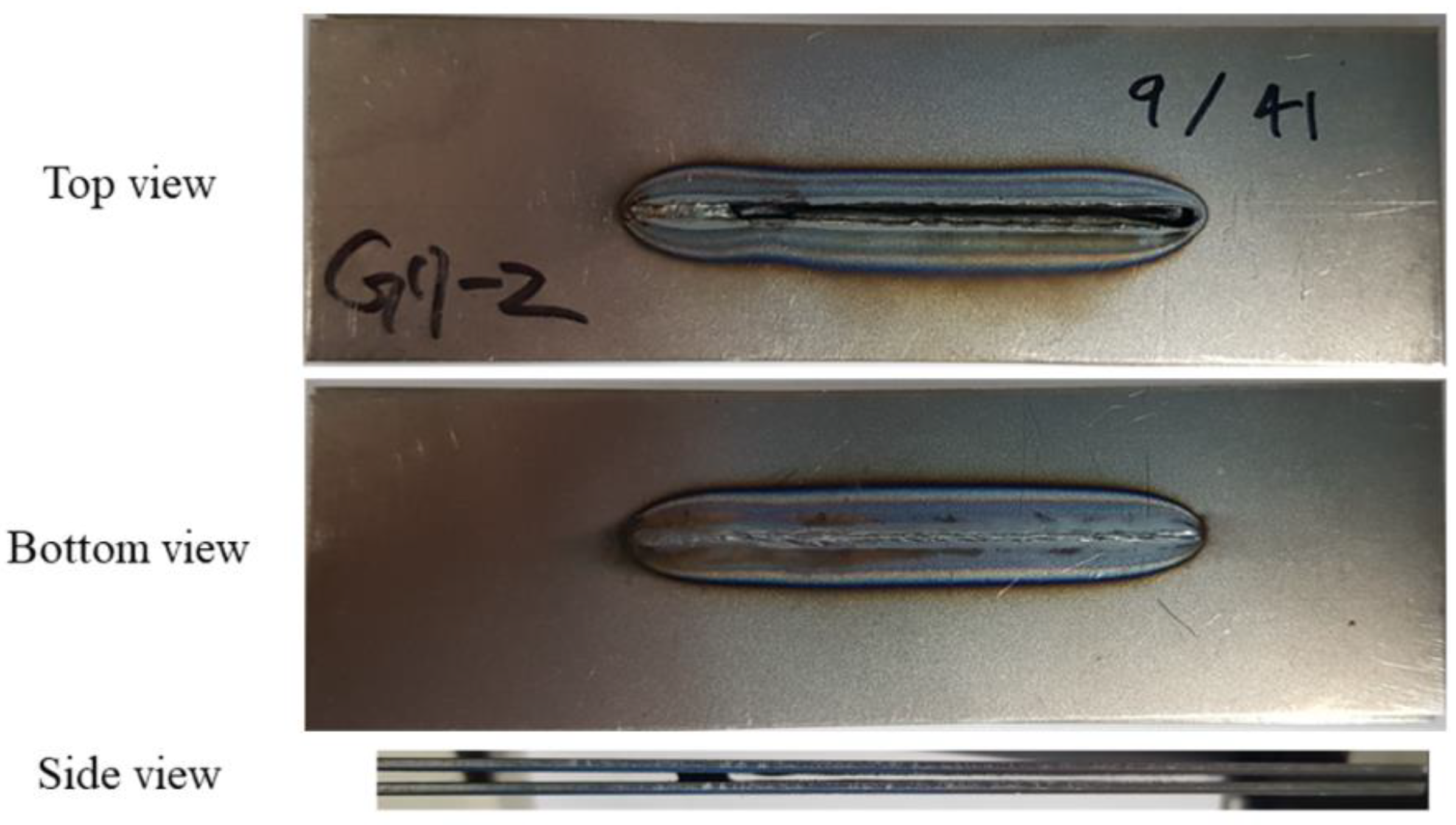
In this study, we evaluated the weld quality, by examining the cross sections of the weld joints, shown in Table 2. Three pre-defined types of joints were observed: unwelded, incomplete penetration, and full penetration, according to different welding speeds and laser power. The “unwelded” type was mainly observed in case of a relatively low power range of 1000–1500 W, and the type “incomplete penetration” was observed in the range of 1500–2000 W. The type “full penetration” was observed in the range of 2500–4000 W. Because the back plate was used in this study (shown in Figure 2), it seems that burn-through was not created when a high laser power was used. That might have led to a larger range of the “full penetration” type. Figure 6 shows the top, bottom, and side views of the weldment, having a gap of 0.8 mm. Although a welding speed of 1.5 m/min and laser power of 3000 W produced a “full penetration” joint, in the case of zero gap (Table 2), a weld joint was not seen, in the case of 0.8 mm gap. This is because the molten metal was insufficient to fill the gap, which was larger in size. This results in the formation of the last type of joint, “unwelded,” which is due to the unfilled gap between the workpieces in the lap joint configuration.
3.2. Signal Analysis
Table 3 shows the color-coded images, which helps to visualize a 3D image of the spectrum intensity (Figure 4) in a 2D form of the spectrum during 0.2 s (0.4–0.6 s). In the color-coded image, the horizontal and vertical axes represent the time and wavelength, respectively, and the intensity is mapped in color. The used color scale was the same used by Viridis [28], and the minimum and maximum values of the color scale were set as 0 and 65535, respectively. It was seen that higher intensities were observed, mainly in the wavelength range of 350–650 nm. In general, when the laser power was kept constant, a higher welding speed increases the intensity. In terms of the size of weld bead, i.e., the penetration and width, this signifies that smaller the weld bead, more was the light, reflected into the spectrometer. Similarly, in case of constant welding speeds, the higher the welding power, the larger was the intensity. However, in this case, even if the size of the weld bead increased, the intensity increased, as the laser power increased. This means that the intensity is influenced more by the laser power, than the weld bead size. These trends were quite clearly observed, in the range of 1000–2500 W of the laser power. However, these trends were rarely observed in all values of laser power more than 3000 W, and rather, all color-coded images in these conditions were almost identical. Additionally, in these conditions, the size of the weld beads, at each welding speed, was almost identical, regardless of the laser power. The growth of the weld bead seems to saturate at a laser power above 3000 W. It is thought that two experimental results, observed when the laser power was more than 3000 W, are related to each other. Table 4 presents the color-coded images of spectrum at all conditions, at a gap of 0.8 mm, and the other configurations except the gap setting are same as those of Table 3. In this case, the pattern of the spectrum intensity was irregular, and the intensity level was smaller, compared to those of Table 3. This result indicates that the irregular geometry of the welding area, caused by the gap, caused a higher irregular reflection of the visible light and laser light. The 3D images (Figure 4) and color-coded images (Table 3 and Table 4) may be difficult to be interpret, and their color and form can also change quite drastically, when compared to a referenced color scale and other configurations. Therefore, in this study, we used the color space created by the International Commission on Illumination in 1931 (CIE 1931 color space), to convert the measured spectrum data to a standard form. The measured spectrum data were converted into CIE 1931 XYZ values, and then these values were further converted into CIE 1931 RGB values by Colour, an open-source Python package, providing algorithms and datasets for color science [29]. The RGB format is effective for showing the features of data measured by the spectrometer and it consists of much smaller data converted using the spectrum data, which allows to estimate models and handle data, with less computation time. Additionally, the maximum value of wavelength for each sample was searched and added.
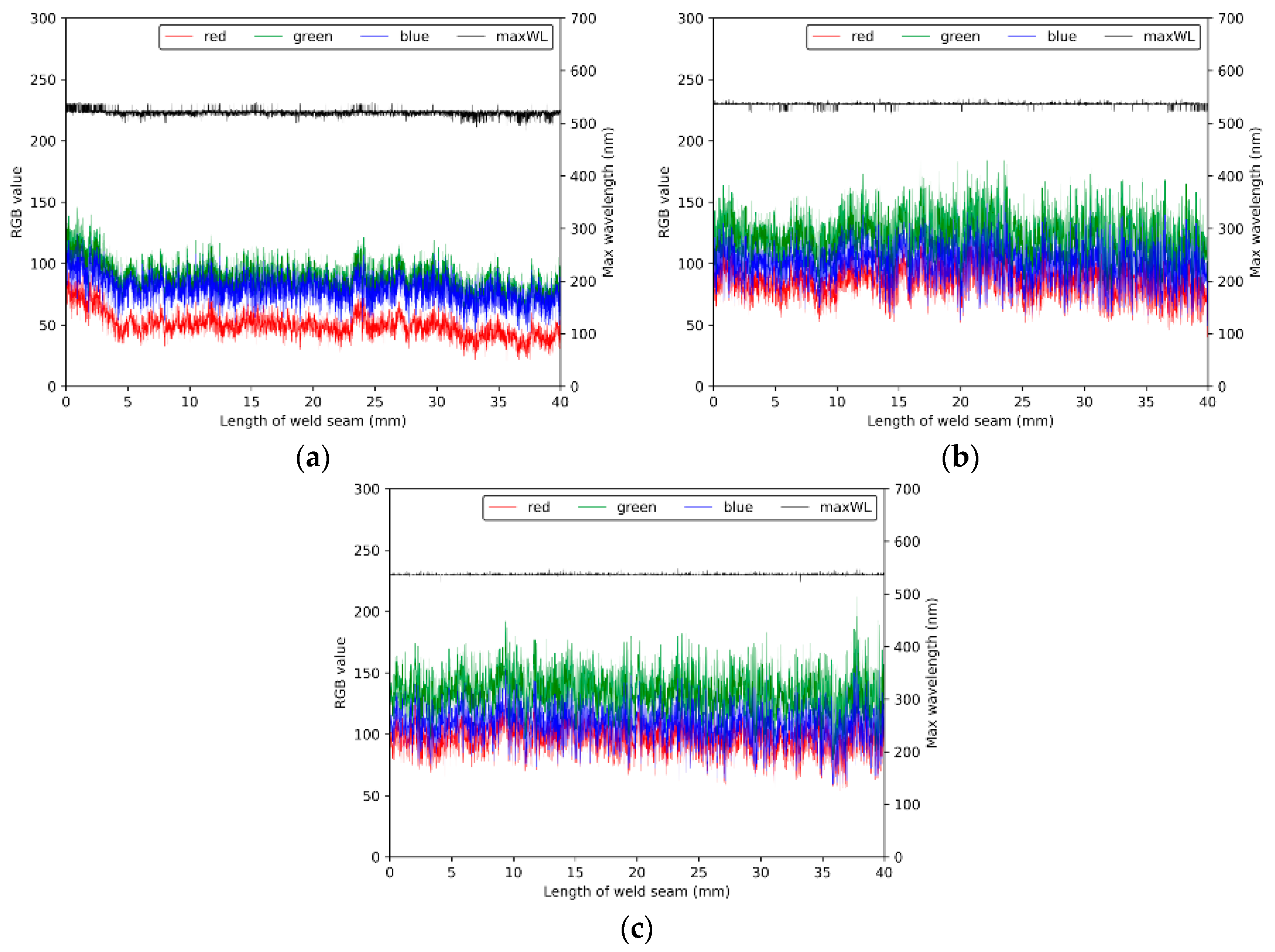
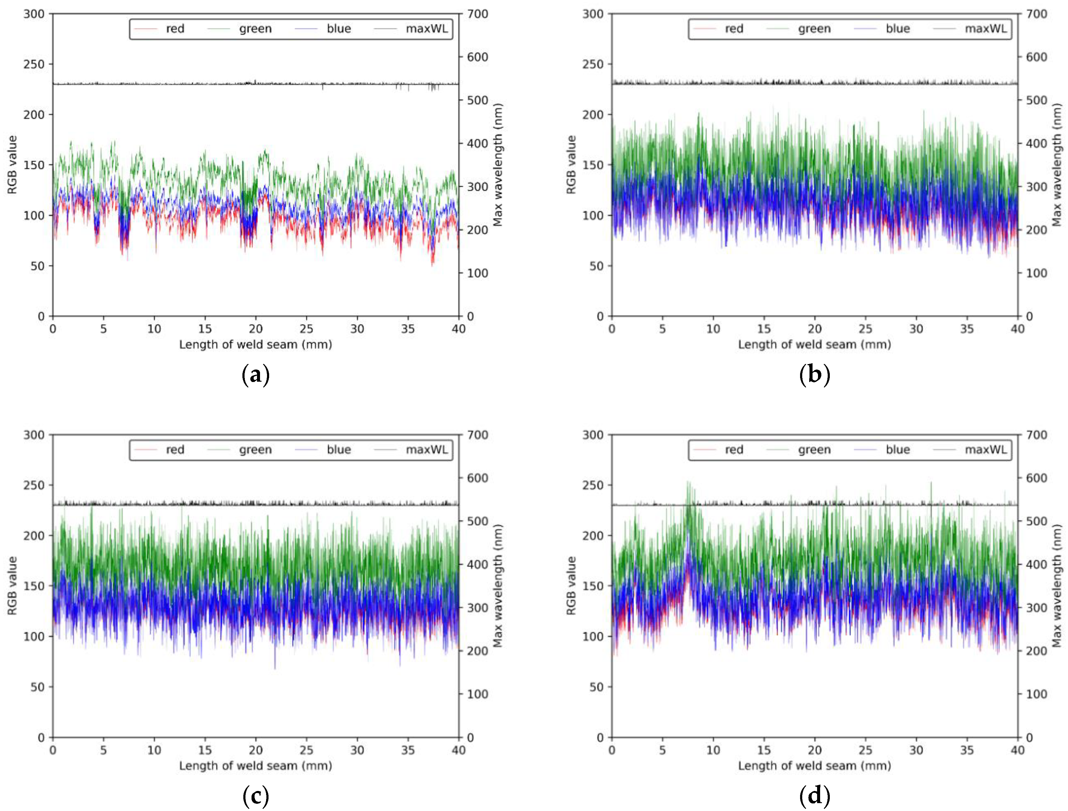
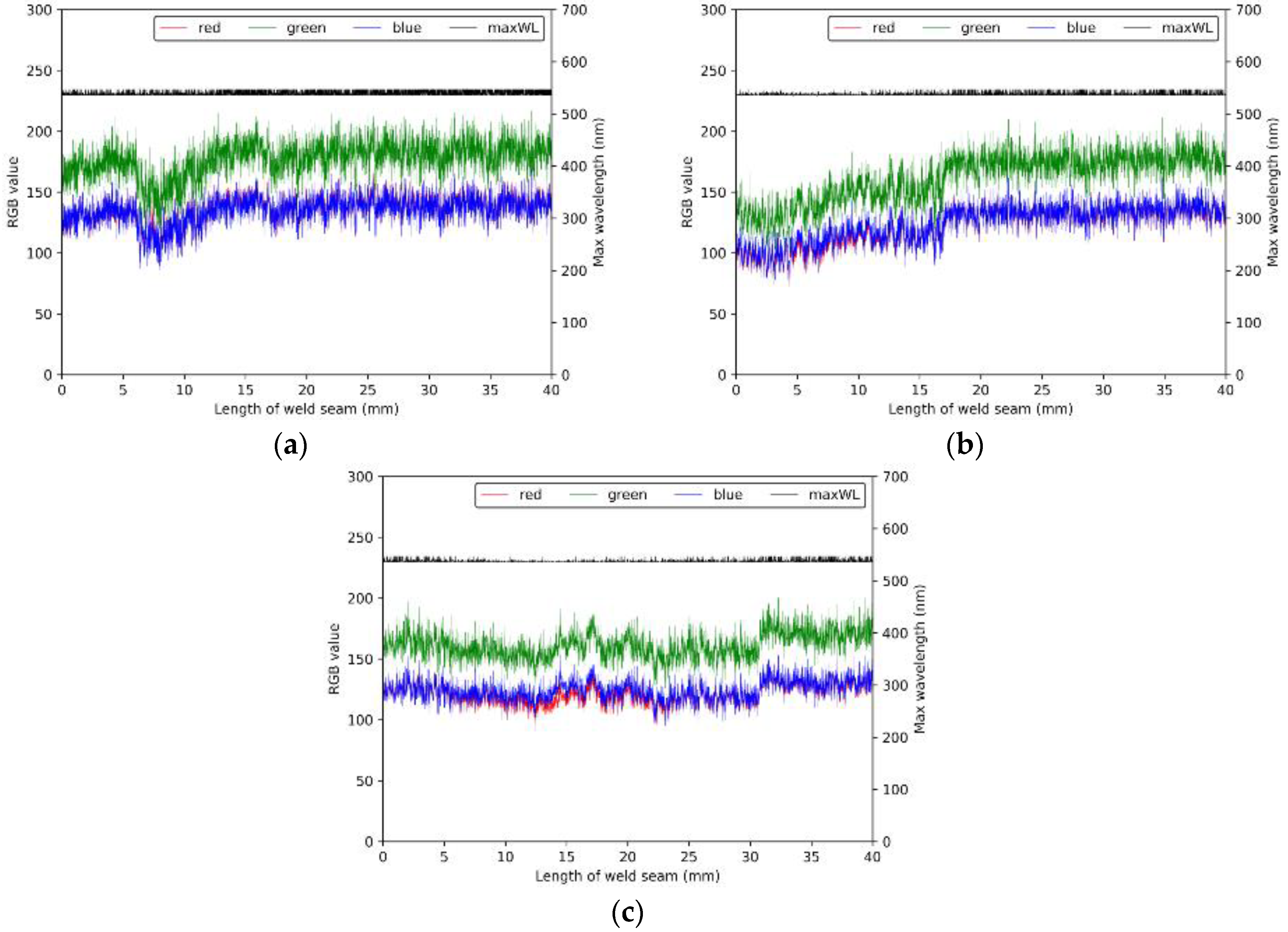
To investigate the effect of the weld penetration on the spectrum intensity, the maximum wavelength and RGB values, at a laser power of 2000 W and different welding speeds, are shown in Figure 7. It is seen that the welding heat input (expressed in kJ/mm) increases, as the welding speed decreases, when the laser power was kept constant. Likewise, the weld penetration increased with increasing heat input, as the welding speed decreased (Table 2). The RGB value, which is converted from the intensity data, decreased when the penetration was increased, which is similar to the results shown in Table 3. It might be inferred that the amount of light reflected from the welding area decreases, as the penetration depth increases, when the laser power is limited to 3000 W, as used in this study. The maximum values of the wavelength were found to be distributed in the range of 500–540 nm, and these values in the case of welding speed 1.5 m/min were slightly lower, when a different welding speed was used. Figure 8 shows the maximum wavelength and RGB values wavelength, at a welding speed of 2.5 m/min, according to different laser powers. The RGB values increased, as the laser power increased, even though the size of weld bead increased due to the high laser power. In addition, the RGB values were almost same, in the conditions of the laser power more than 3000 W. These results were found to be in good agreement, with those of Table 3. The maximum values of wavelength were distributed in the range of 530–540 nm. Figure 9 shows the RGB values and maximum wavelength at a gap of 0.8 mm, and a 3000 W laser power, according to the welding speed. In this case, the maximum wavelength and RGB values were almost same as those shown in Figure 8c, which had conditions of a 3000 W laser power and a 2.5 m/min welding speed. However, overall waveforms of the RGB curves were found to be uneven and irregularly-shaped, and the variations of the RGB and maximum wavelength values were relatively small, as compared to those of the cases when the laser power was above 3000 W. For this reason, the green curve is clearly separated from the red and blue curves, as seen in Figure 9.
3.3. Weld Quality Prediction Model
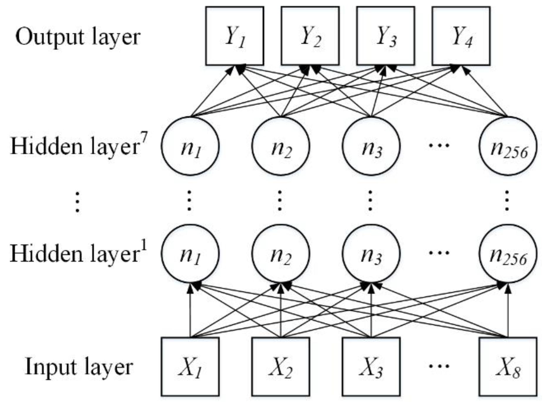
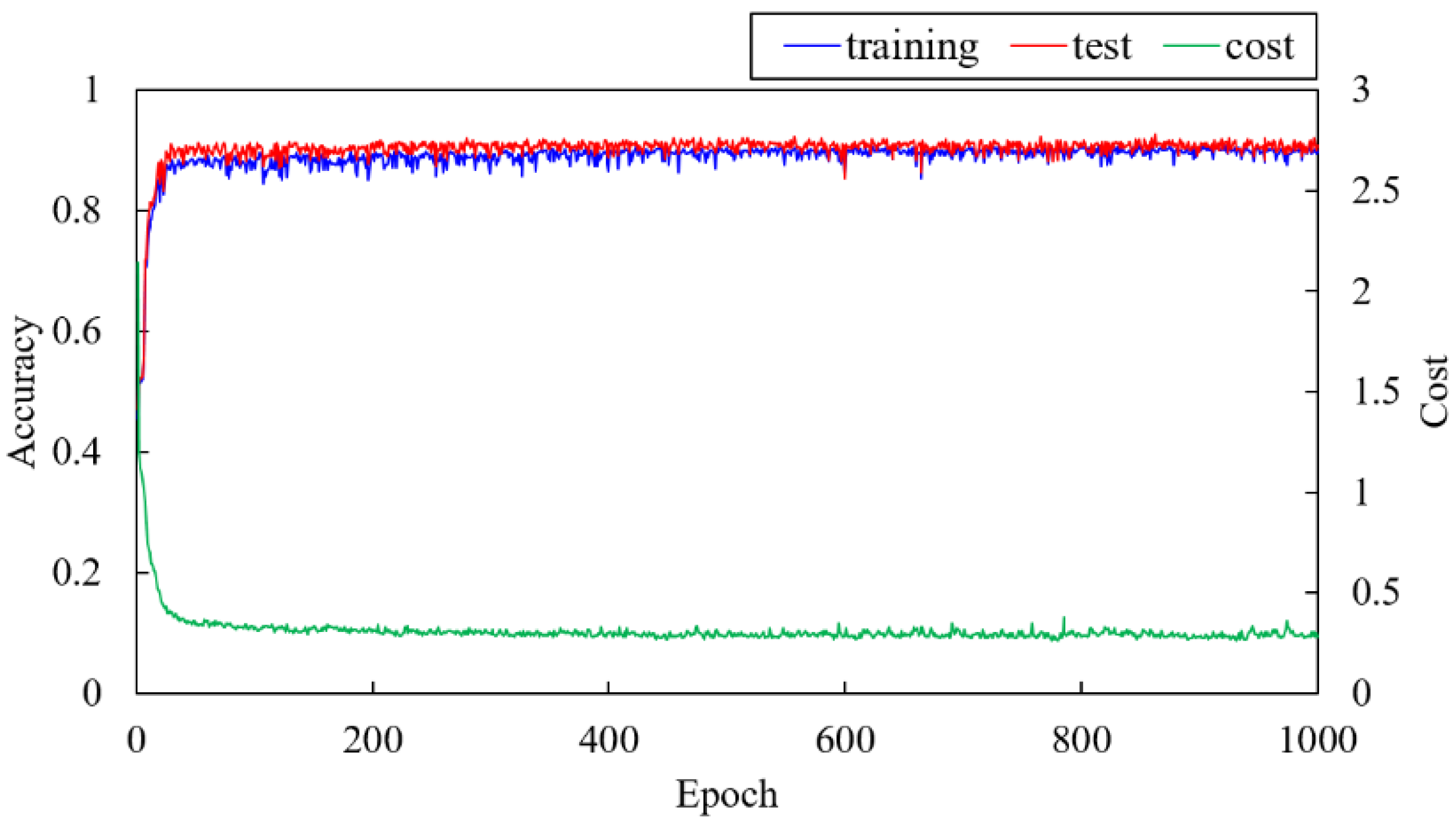
To predict the weld quality, a DNN model was used as the prediction model. As shown in Figure 10, we modeled a neural architecture, as a seven-hidden-layer DNN, and assigned 256 neurons to each of the hidden layer. The neurons of every preceding layer were fully connected, to those of the succeeding layer. The eight values, which were the average and standard deviation of the RGB values and the maximum wavelength, were used as the inputs to the network (see Nomenclature). Especially, considering the weld size and speed of welding, the model was designed to predict the weld quality, per 0.5 mm of the weld length. The outputs are the four joint types, described in Section 2.3: unwelded (Y1), incomplete penetration (Y2), full penetration (Y3), and unwelded by a gap (Y4). The other specifications of the DNN implementation model is summarized in Table 5. All the hidden layers utilized rectified linear unit (ReLU) functions, to calculate their respective intermediate outputs. The output layer had four nodes, and the output layer with the Softmax activation function computed and returned the type probability with respect to each of the output types. The prediction of the weld quality, by the model, was determined based on the type probability. A total of 5400 data sets (4320 training sets and 1080 test sets) were used to generate the DNN model. Each dataset contained the given eight input variables, and four output variables. The backpropagation algorithms were carried out with a batch size of 50, with 500 epochs. Figure 11 shows the training results, including the cost, training accuracy, and test accuracy. After training, the cost value was calculated as 0.2806, the training accuracy was 0.8993, and the test accuracy was 0.9083.
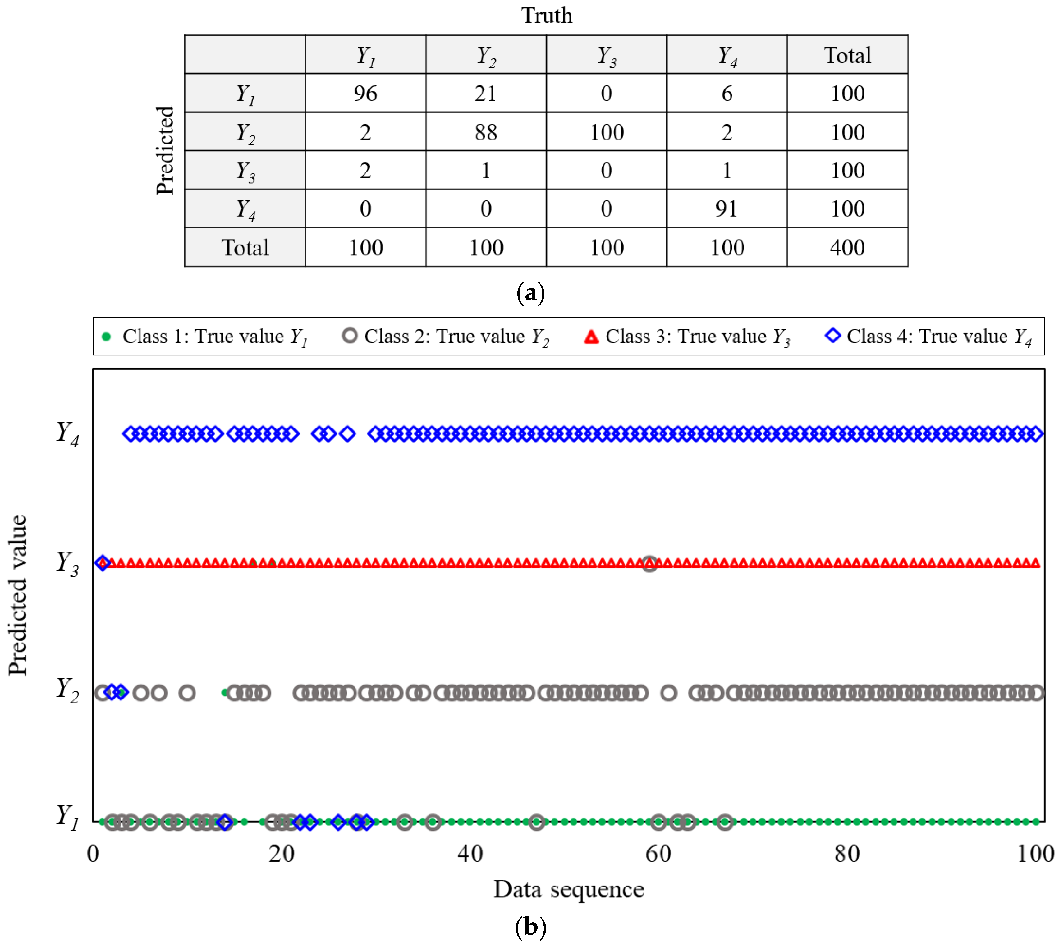
To test the developed model, we produced 100 test datasets, for each class, by carrying out an additional welding experiment. Figure 12 shows the result of testing the developed DNN model using 400 test datasets, the confusion matrix and prediction result according to weld seam length. In Figure 12, the vertical and horizontal axes represent the predicted value of the DNN model and the data sequence, respectively. The four symbols, green, gray, red, and blue, represent the class to which each dataset belongs. It is seen that most of the errors occurred owing to the false prediction of Y2 as Y1. That is, 22 of the 100 datasets of class 2 (Y2) made false predictions, and among them, the 21 datasets were predicted as class 1 (Y1). Although Y1 and Y2 are divided into unwelded and incomplete penetration, respectively, in this study, Y1 and Y2 can be the same case, which is not full penetration. In particular, in the lap joint configuration of the two same metal sheets, if the penetration depth is less than 50% of the sum of the thickness of the two sheets, the weld quality is classified Y1. If the penetration depth is more than 50% but less than the sum of thickness of the two sheets, the weld quality is classified Y2. It is considered that this relationship between Y1 and Y2 causes this error. In addition, most errors occurred at the beginning of welding, which could be due to the relatively unstable spectral signal at the beginning of welding. In the case of Y4, 9 of the 100 datasets made false predictions. The errors, which occur, by predicting Y4 as the other classes, might be due to excessively irregular signal of Y4. In the case of Y3, there is no error in predicting the weld quality because its signal was stable and had a distinct distribution in the RGB space. In summary, the biggest prediction error was seen to have occurred in predicting Y2. This error could be explained by the relatively small amount of available training data needed to increase the prediction accuracy of Y2. That is, it is assumed that there were insufficient training data that otherwise could have made the quality prediction model more accurate in classifying Y2 and Y1. As presented in Table 3 and Table 4, the range of the welding conditions in which the data for Y2 can be obtained is smaller than that of other classes, and these welding conditions exist in the range of laser power of 1500–2000 W. If sufficient training data is obtained through more detailed experiments in the same range of laser power, the obtained data can reduce the prediction errors by more clearly learning a prediction model the boundary of Y2 and Y1.
4. Conclusions
In this study, we proposed the DNN-based quality assessment method based on a spectrometer in the LBW process, conducted the relevant experiments to analyze the features of the measured data, and verified the developed method. Notable developments and outcomes from this study are as follows.
- We designed and developed a spectrometer that can measure and analyze the light reflected from the welding area in an LBW process. The spectral response range of the developed spectrometer was 225–975 nm, and its sampling frequency was 5 kHz.
- The spectral data were converted to the CIE 1931 RGB color space to analyze the features of the spectral data and obtain the standardized and simplified spectral data.
- The prediction model that can classify the weld quality for LBW using data measured by the spectrometer was also developed. The weld quality prediction model was designed based on DNN, and the DNN model was trained using the converted RGB data and maximum frequency values. The developed model had a weld quality prediction accuracy of approximately 90%.
The results of this study substantially contribute to the state-of-the-art, regarding the automation of the welding process and monitoring technology, for LBW processes. Despite our study’s contributions, some limitations are worth noting. Although our quality prediction model, based on the spectrometer, effectively estimates the weld quality of laser welding, the application of the model is limited to the scope of this study. Future work will focus on the generalization of the quality assessment method proposed in this study. For this purpose, we will collect sufficient data on various materials and welding conditions, and then further improve the data processing techniques and quality assessment algorithms using advanced ML algorithms. In parallel, we will also improve our spectrometer and its software developed in this study.
Author Contributions
The research presented here was carried out in collaboration between all authors. Conceptualization, M.K., I.H. and H.L.; data curation, D.-Y.K. and J.Y.; formal analysis, J.Y. and D.-Y.K.; investigation, J.Y. and D.-Y.K.; methodology, J.Y.; software, H.L. and J.Y.; validation, J.Y. and D.-Y.K.; writing—original draft, J.Y.; writing—review and editing, M.K. and J.Y.; funding acquisition, I.H.; supervision, I.H. and H.L.; project administration, M.K. All authors have read and agreed to the published version of the manuscript.
Funding
This work was supported by funding from the Korea Institute of Industrial Technology.
Acknowledgments
This study has been conducted with the support of the Korea Institute of Industrial Technology as “Development of intelligent root technology with add-on modules (kitech EO-20-0017)”.
Conflicts of Interest
The authors declare no conflict of interest.
Nomenclature
| ML | Machine learning |
| LBW | Laser beam welding |
| RSM | Response surface methodology |
| SVM | Support vector machine |
| ANN | Artificial neural network |
| GA | Genetic algorithm |
| SSAE | Stacked sparse autoencoder |
| DNN | Deep neural network |
| CMOS | Complementary metal-oxide-semiconductor |
| DP | DP Dual phase |
| Ar | Argon |
| CIE | International commission on illumination |
| ReLU | Rectified linear unit |
| X1 | Average value of red light during per 0.5 mm of weld length |
| X2 | Standard deviation of red light per 0.5 mm of weld length |
| X3 | Average value green light per 0.5 mm of weld length |
| X4 | Standard deviation of green light per 0.5 mm of weld length |
| X5 | Average value blue light per 0.5 mm of weld length |
| X6 | Standard deviation of blue light per 0.5 mm of weld length |
| X7 | Average value of the maximum wavelength per 0.5 mm of weld length |
| X8 | Standard deviation of blue light per 0.5 mm of weld length |
| Y1 | Unwelded (Class 1) |
| Y2 | Incomplete penetration (Class 2) |
| Y3 | Full penetration (Class 3) |
| Y4 | Unwelded by a gap (Class 4) |
References
- Tmforum. Available online: https://inform.tmforum.org/archive/2020/03/the-fourth-industrial-revolution-manufacturing-and-beyond/ (accessed on 4 June 2020).
- Chryssolouris, G.; Papakostas, N.; Mavrikios, D. A perspective on manufacturing strategy: Produce more with less. CIRP J Manuf. Sci. Technol. 2008, 1, 45–52. [Google Scholar] [CrossRef]
- Abdullah, H.A.; Siddiqui, R.A. Concurrent laser welding and annealing exploiting robotically manipulated optical fibers. Opt. Laser Eng. 2002, 38, 473–484. [Google Scholar] [CrossRef]
- Tsoukantas, G.; Salonitis, K.; Stournaras, A.; Stavropoulos, P.; Chryssolouris, G. On optical design limitations of generalized two-mirror remote beam delivery laser systems: The case of remote welding. Int. J. Adv. Manuf. Technol. 2007, 32, 932–941. [Google Scholar] [CrossRef]
- Mohammed, G.R.; Ishak, M.; Ahmad, S.N.A.S.; Abdulhadi, H.A. Fiber laser welding of dissimilar 2205/304 stainless steel plates. Metals 2017, 7, 546. [Google Scholar] [CrossRef] [Green Version]
- Javaheri, E.; Lubritz, J.; Graf, B.; Rethmeier, M. Mechanical properties characterization of welded automotive steels. Metals 2020, 10, 1. [Google Scholar] [CrossRef] [Green Version]
- Zeng, Z.; Oliveira, J.P.; Yang, M.; Song, D.; Peng, B. Functional fatigue behavior of NiTi-Cu dissimilar laser welds. Mater. Des. 2017, 114, 282–287. [Google Scholar] [CrossRef]
- Oliveira, J.P.; Fernandes, F.M.B.; Schell, N.; Miranda, R.M. Shape memory effect of laser welded NiTi plates. Funct. Mater. Lett. 2015, 8, 1550069. [Google Scholar] [CrossRef]
- Zeng, Z.; Yang, M.; Oliveira, J.P.; Song, D.; Peng, B. Laser welding of NiTi shape memory alloy wires and tubes for multi-functional design applications. Smart Mater. Struct. 2016, 25, 085001. [Google Scholar] [CrossRef]
- Stavridis, J.; Papacharalampopoulos, A.; Stavropoulos, P. Quality assessment in laser welding: A critical review. Int. J. Adv. Manuf. Technol. 2018, 94, 1825–1847. [Google Scholar] [CrossRef]
- Stournaras, A.; Stavropoulos, P.; Salonitis, K.; Chryssolouris, G. Laser process monitoring: A critical review. In Proceedings of the 6th International Conference on Manufacturing Research, Uxbridge, UK, 9–11 September 2008; pp. 425–435. [Google Scholar]
- Huang, W.; Kovacevic, R. A laser-based vision system for weld quality inspection. Sensors 2011, 11, 506–521. [Google Scholar] [CrossRef]
- Kim, C.-H.; Ahn, D.-C. Coaxial monitoring of keyhole during Yb:YAG laser welding. Opt. Laser Technol. 2012, 44, 1874–1880. [Google Scholar] [CrossRef]
- Gao, X.-D.; Wen, Q.; Katayama, S. Analysis of high-power disk laser welding stability based on classification of plume and spatter characteristics. Trans. Nonferrous. Metals Soc. China 2013, 23, 3748–3757. [Google Scholar] [CrossRef]
- Purtonen, T.; Kalliosaari, A.; Salminen, A. Monitoring and adaptive control of laser processes. Phys. Procedia 2014, 56, 1218–1231. [Google Scholar] [CrossRef] [Green Version]
- Zeng, H.; Zhou, Z.; Chen, Y.; Luo, H.; Hu, L. Wavelet analysis of acoustic emission signals and quality control in laser welding. J. Laser Appl. 2001, 13, 167–173. [Google Scholar] [CrossRef]
- Du, D.; Cai, G.-R.; Tian, Y.; Hou, R.-S.; Wang, L. Automatic inspection of weld defects with x-ray real-time imaging. Lect. Notes Contrib. Inf. 2007, 362, 359–366. [Google Scholar]
- Park, Y.W.; Park, H.; Rhee, S.; Kang, M. Real time estimation of CO2 laser weld quality for automotive industry. Opt. Laser Technol. 2002, 34, 135–142. [Google Scholar] [CrossRef]
- Sibillano, T.; Ancona, A.; Berardi, V.; Schingaro, E.; Parente, P.; Lugarà, P.M. Correlation spectroscopy as a tool for detecting losses of ligand elements in laser welding of aluminium alloys. Opt Laser Eng. 2006, 44, 1324–1335. [Google Scholar] [CrossRef]
- Rizzi, D.; Sibillano, T.; Pietro Calabrese, P.; Ancona, A.; Mario Lugarà, P. Spectroscopic, energetic and metallographic investigations of the laser lap welding of AISI 304 using the response surface methodology. Opt Laser Eng. 2011, 49, 892–898. [Google Scholar] [CrossRef]
- Konuk, A.R.; Aarts, R.G.K.M.; Veld, A.J.H.; Sibillano, T.; Rizzi, D.; Ancona, A. Process control of stainless steel laser welding using an optical spectroscopic sensor. Phys. Procedia 2011, 12, 744–751. [Google Scholar] [CrossRef] [Green Version]
- Sebestova, H.; Chmelickova, H.; Nozka, L.; Moudry, J. Non-destructive real time monitoring of the laser welding process. J. Mater. Eng. Perform. 2012, 21, 764–769. [Google Scholar] [CrossRef]
- Zaeh, M.F.; Huber, S. Characteristic line emissions of the metal vapour during laser beam welding. Prod. Eng. 2011, 5, 667–678. [Google Scholar] [CrossRef]
- Chen, Y.; Chen, B.; Yao, Y.; Tan, C.; Feng, J. A spectroscopic method based on support vector machine and artificial neural network for fiber laser welding defects detection and classification. NDT E Int. 2019, 108, 102176. [Google Scholar] [CrossRef]
- Zhang, Y.; You, D.; Gao, X.; Wang, C.; Li, Y.; Gao, P.P. Real-time monitoring of high-power disk laser welding statuses based on deep learning framework. J. Intell. Manuf. 2020, 31, 799–814. [Google Scholar] [CrossRef]
- Lee, S.H.; Mazumder, J.; Park, J.; Kim, S. Ranked Feature-Based Laser Material Processing Monitoring and Defect Diagnosis Using k-NN and SVM. J. Manuf. Process. 2020, 55, 307–316. [Google Scholar] [CrossRef]
- You, D.; Gao, X.; Katayama, S. Multiple-optics sensing of high-brightness disk laser welding process. NDT E Int. 2013, 60, 32–39. [Google Scholar]
- CRAN. Available online: https://cran.r-project.org/web/packages/viridis/vignettes/intro-to-viridis.html/ (accessed on 4 June 2020).
- COLOUR. Available online: https://colour.readthedocs.io/en/develop/ (accessed on 4 June 2020).
Figure 1.
Configuration of the developed spectrometer: (a) schematic; (b) designed prototype.

Figure 2.
Schematic of experimental setup.

Figure 3.
Experimental setup and installation of the spectrometer.

Figure 4.
Spectrum intensity variation, in the LBW of a lap joint configuration, with a welding speed 1.5 m/min and a laser power of 3500 W (thickness of sheet is 1.2 mm).
Figure 4.
Spectrum intensity variation, in the LBW of a lap joint configuration, with a welding speed 1.5 m/min and a laser power of 3500 W (thickness of sheet is 1.2 mm).

Figure 5.
Schematics of four weld qualities defined in this study.

Figure 6.
Workpiece appearance with a gap of 0.8 mm after welding with a welding speed 1.5 m/min and a laser power of 3000 W: top view, bottom view, side view.
Figure 6.
Workpiece appearance with a gap of 0.8 mm after welding with a welding speed 1.5 m/min and a laser power of 3000 W: top view, bottom view, side view.

Figure 7.
RGB values and maximum wavelength at laser power of 2000 W: welding speed of (a) 1.5 m/min; (b) 2.0 m/min; (c) 2.5 m/min.
Figure 7.
RGB values and maximum wavelength at laser power of 2000 W: welding speed of (a) 1.5 m/min; (b) 2.0 m/min; (c) 2.5 m/min.

Figure 8.
RGB values and maximum wavelength at welding speed of 2.5 m/min: laser power of (a) 1000 W; (b) 2000 W; (c) 3000 W; (d) 4000 W.
Figure 8.
RGB values and maximum wavelength at welding speed of 2.5 m/min: laser power of (a) 1000 W; (b) 2000 W; (c) 3000 W; (d) 4000 W.

Figure 9.
RGB values and maximum wavelength, at 0.8 mm gap and 3000 W laser power: welding speed of (a) 1.5 m/min; (b) 2.0 m/min; (c) 2.5 m/min.
Figure 9.
RGB values and maximum wavelength, at 0.8 mm gap and 3000 W laser power: welding speed of (a) 1.5 m/min; (b) 2.0 m/min; (c) 2.5 m/min.

Figure 10.
Structure of the deep neural network (DNN) model to classify the weld quality.

Figure 11.
Training results: training accuracy, test accuracy, and cost.

Figure 12.
Verification results: (a) confusion matrix; (b) prediction result according to data sequence.
Figure 12.
Verification results: (a) confusion matrix; (b) prediction result according to data sequence.


Table 1.
Experimental factors and their values.
| Welding Parameter | Value |
|---|---|
| Laser power (W) | 1000, 1500, 2000, 2500, 3000, 3500, 4000 |
| Welding speed (m/min) | 1.5, 2.0, 2.5 |
| Gap (mm) | 0, 0.8 |
Table 2.
Cross-sections of welded joint according to the laser power and welding speed.
| Laser Power (W) | Welding Speed (m/min) | ||
|---|---|---|---|
| 1.5 | 2.0 | 2.5 | |
| 1000 | Unwelded | Unwelded | Unwelded |
| 1500 |  | Unwelded | Unwelded |
| 2000 |  |  |  |
| 2500 |  |  |  |
| 3000 |  |  |  |
| 3500 |  |  |  |
| 4000 |  |  |  |
Table 3.
Color-coded images of spectrum, according to the laser power and welding speed; in each image, the horizontal axis is time (s), the vertical axis is wavelength (nm), and intensity is mapped in color (color scale: Viridis, date from [28]).
Table 3.
Color-coded images of spectrum, according to the laser power and welding speed; in each image, the horizontal axis is time (s), the vertical axis is wavelength (nm), and intensity is mapped in color (color scale: Viridis, date from [28]).
| Laser Power (W) | Welding Speed (m/min) | Color Scalelegend | ||
|---|---|---|---|---|
| 1.5 | 2.0 | 2.5 | ||
| 1000 |  |  |  |  |
| 1500 |  |  |  |  |
| 2000 |  |  |  |  |
| 2500 |  |  |  |  |
| 3000 |  |  |  |  |
| 3500 |  |  |  |  |
| 4000 |  |  |  |  |
Table 4.
Color-coded images of spectrum at a gap of 0.8 mm according to the laser power and welding speed: in each image, the horizontal axis is time (s), the vertical axis is wavelength (nm), and intensity is mapped in color (color scale: Viridis, data from [28]).
Table 4.
Color-coded images of spectrum at a gap of 0.8 mm according to the laser power and welding speed: in each image, the horizontal axis is time (s), the vertical axis is wavelength (nm), and intensity is mapped in color (color scale: Viridis, data from [28]).
| Laser Power (W) | Welding Speed (m/min) | Color Scalelegend | ||
|---|---|---|---|---|
| 1.5 | 2.0 | 2.5 | ||
| 3000 |  |  |  |  |
| 4000 |  |  |  |  |
Table 5.
Summary of DNN model implementation.
| Item | Description | ||
|---|---|---|---|
| Structure | Input Layer | Hidden Layer | Output Layer |
| Number of nodes | 8 | 256 | 4 |
| Learning rate | 0.001 | ||
| Epoch | 1000 | ||
| Batch size | 100 | ||
| Activation function | ReLU | ||
| Function of output layer | Softmax | ||
| Cost function | Cross-entropy | ||
| Optimizer | Adam optimizer | ||
© 2020 by the authors. Licensee MDPI, Basel, Switzerland. This article is an open access article distributed under the terms and conditions of the Creative Commons Attribution (CC BY) license (http://creativecommons.org/licenses/by/4.0/).
Share and Cite
MDPI and ACS Style
Yu, J.; Lee, H.; Kim, D.-Y.; Kang, M.; Hwang, I. Quality Assessment Method Based on a Spectrometer in Laser Beam Welding Process. Metals 2020, 10, 839. https://0-doi-org.brum.beds.ac.uk/10.3390/met10060839
AMA Style
Yu J, Lee H, Kim D-Y, Kang M, Hwang I. Quality Assessment Method Based on a Spectrometer in Laser Beam Welding Process. Metals. 2020; 10(6):839. https://0-doi-org.brum.beds.ac.uk/10.3390/met10060839
Chicago/Turabian StyleYu, Jiyoung, Huijun Lee, Dong-Yoon Kim, Munjin Kang, and Insung Hwang. 2020. "Quality Assessment Method Based on a Spectrometer in Laser Beam Welding Process" Metals 10, no. 6: 839. https://0-doi-org.brum.beds.ac.uk/10.3390/met10060839
Note that from the first issue of 2016, this journal uses article numbers instead of page numbers. See further details here.