Estimation of Heat Source Model’s Parameters for GMAW with Non-linear Global Optimization—Part I: Application of Multi-island Genetic Algorithm


Abstract
:1. Introduction
2. Background
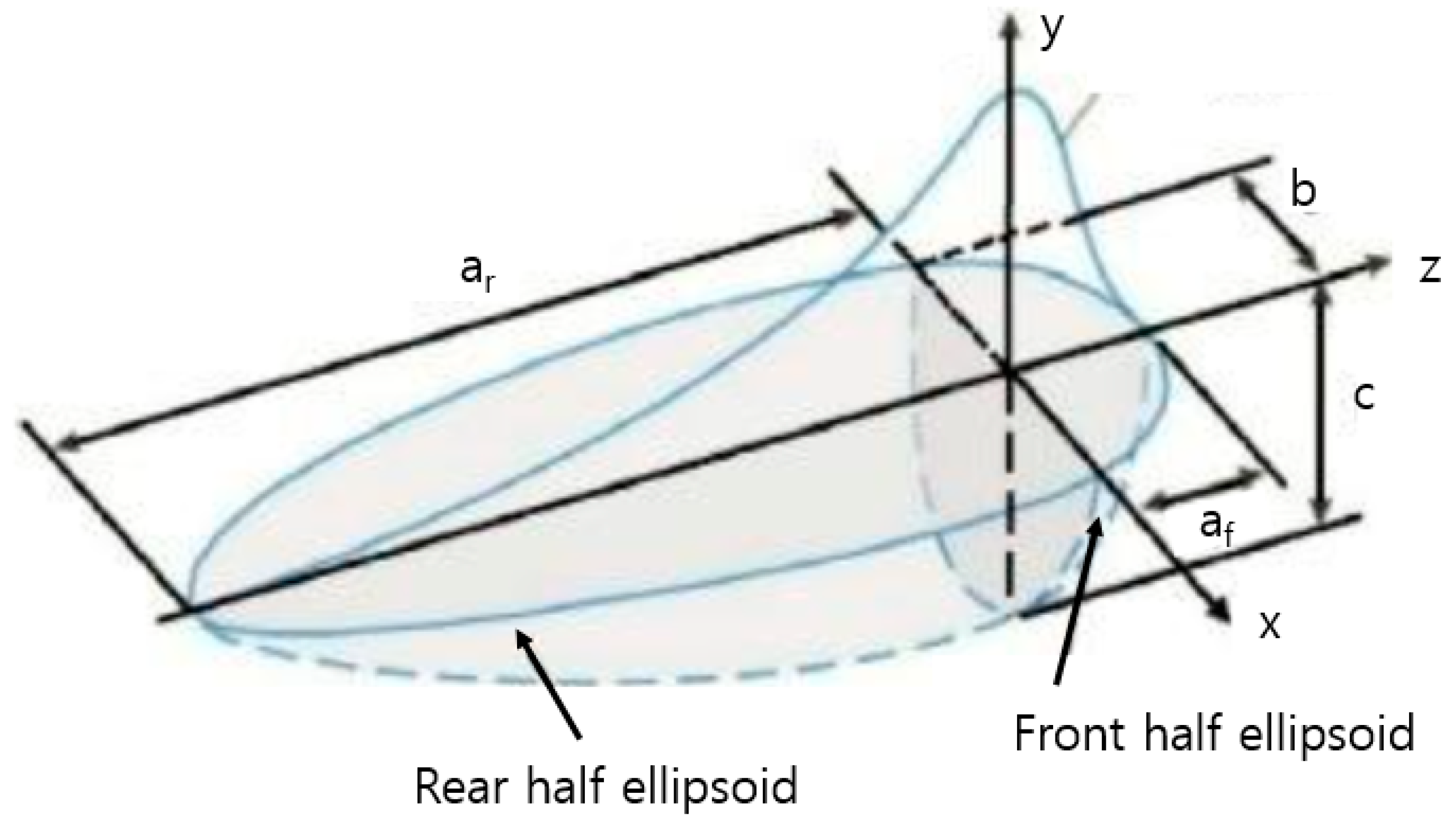
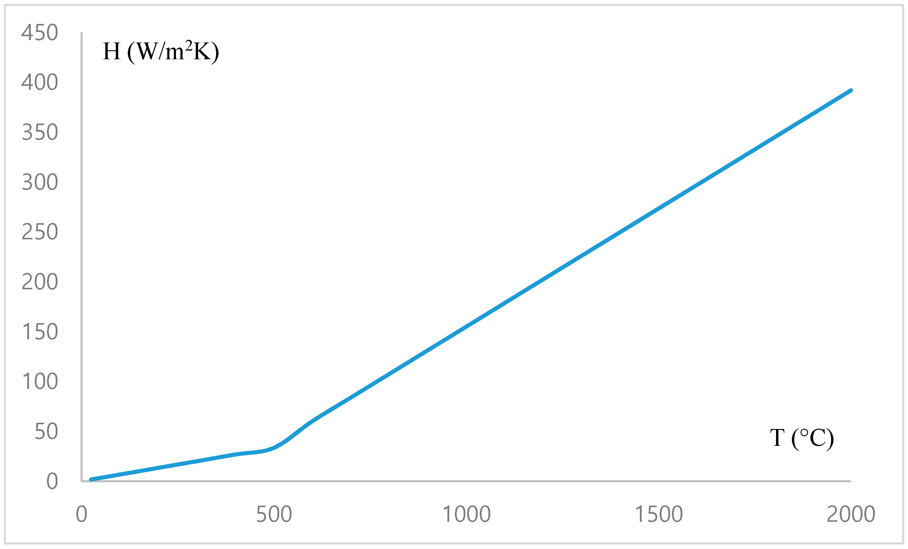
2.1. Heat Source Model
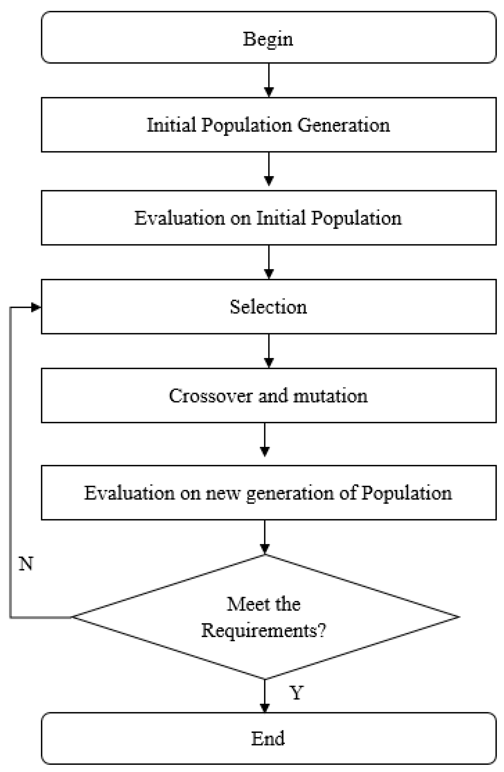
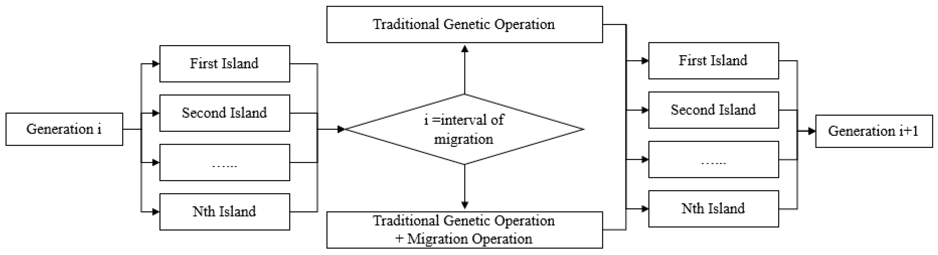
2.2. Global Optimization Algorithm
3. Experiment
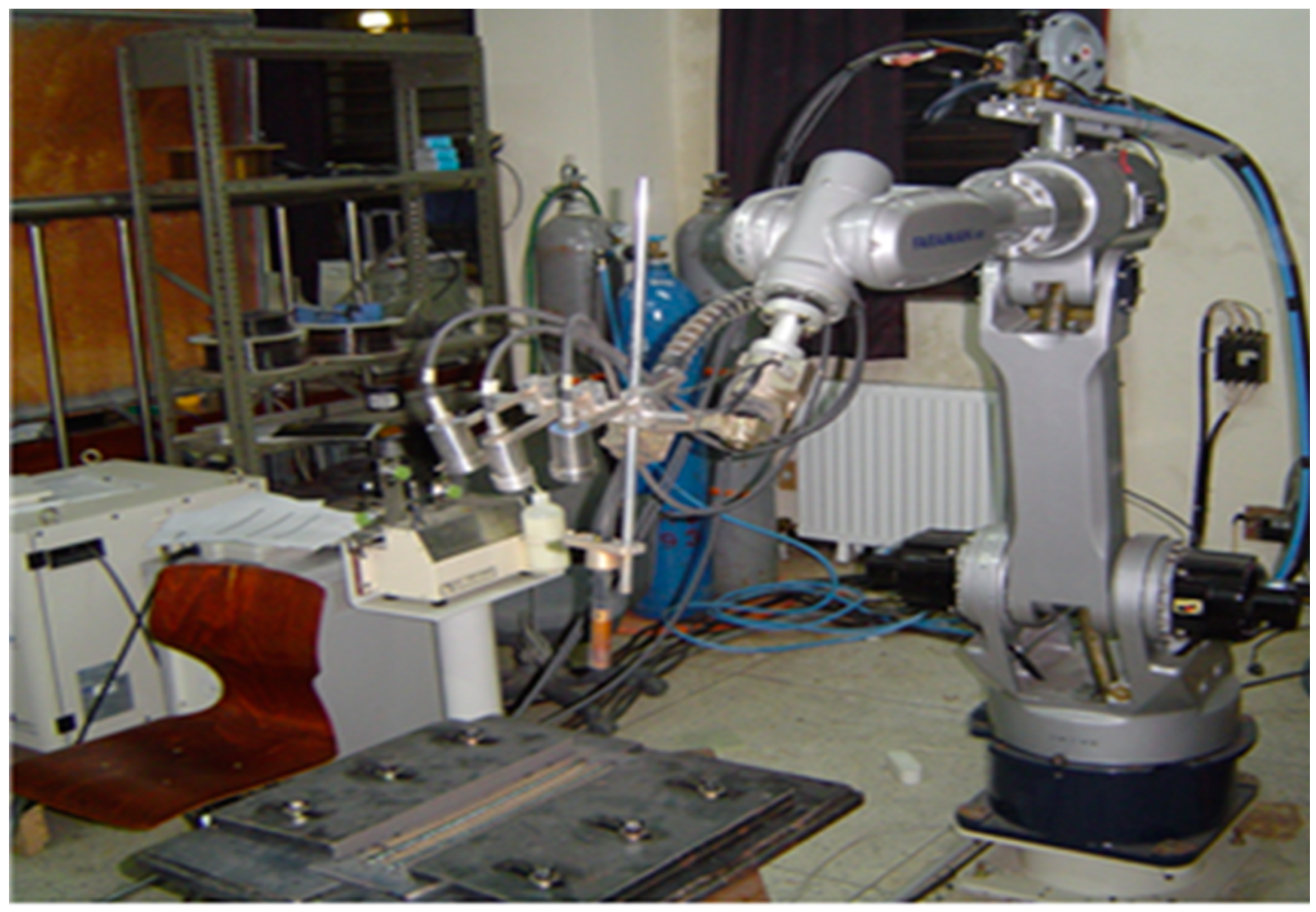
3.1. Experiment Setup
3.2. Experiment Condition
3.3. Experiment Result and Data Measurement
4. Numerical Simulation
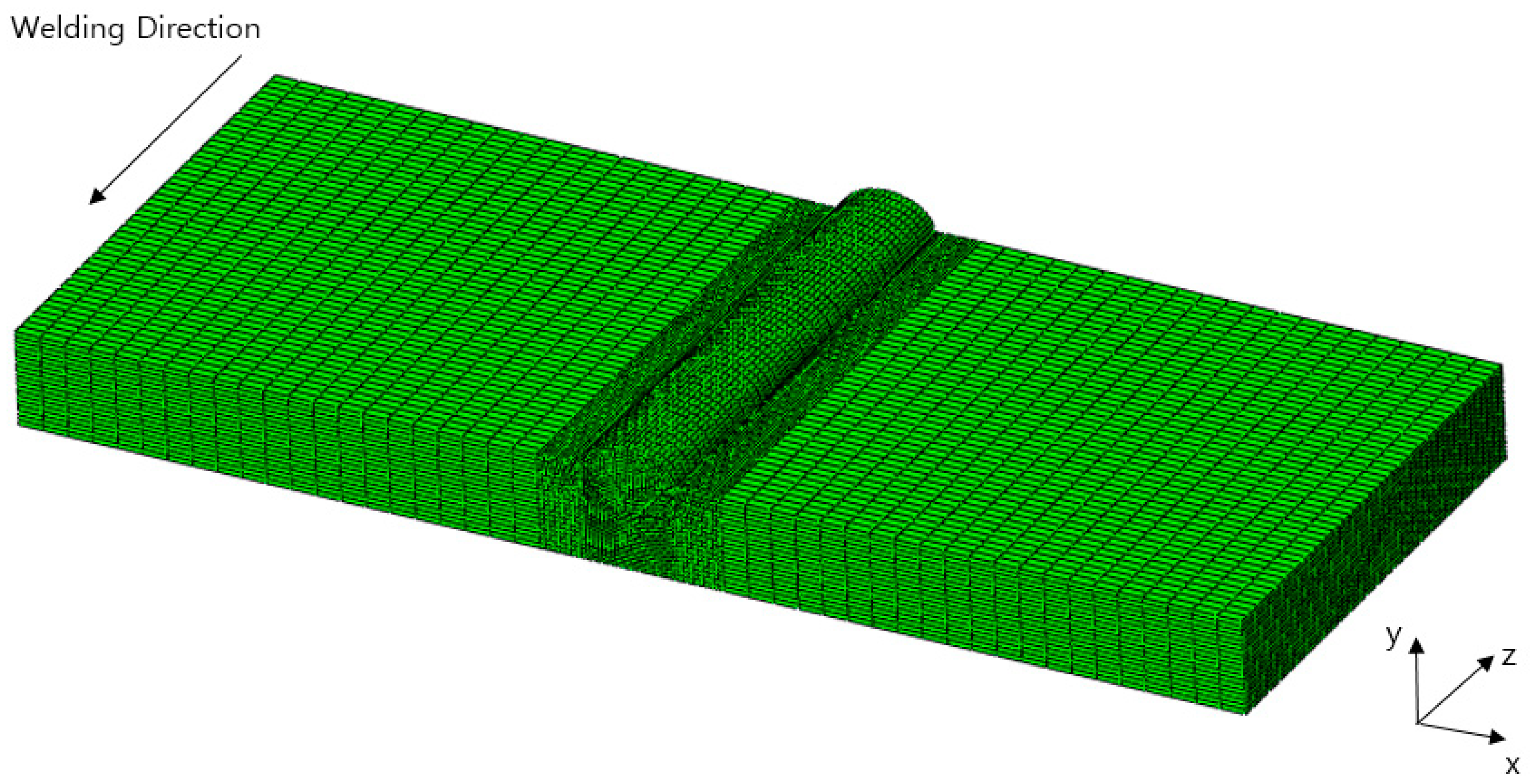
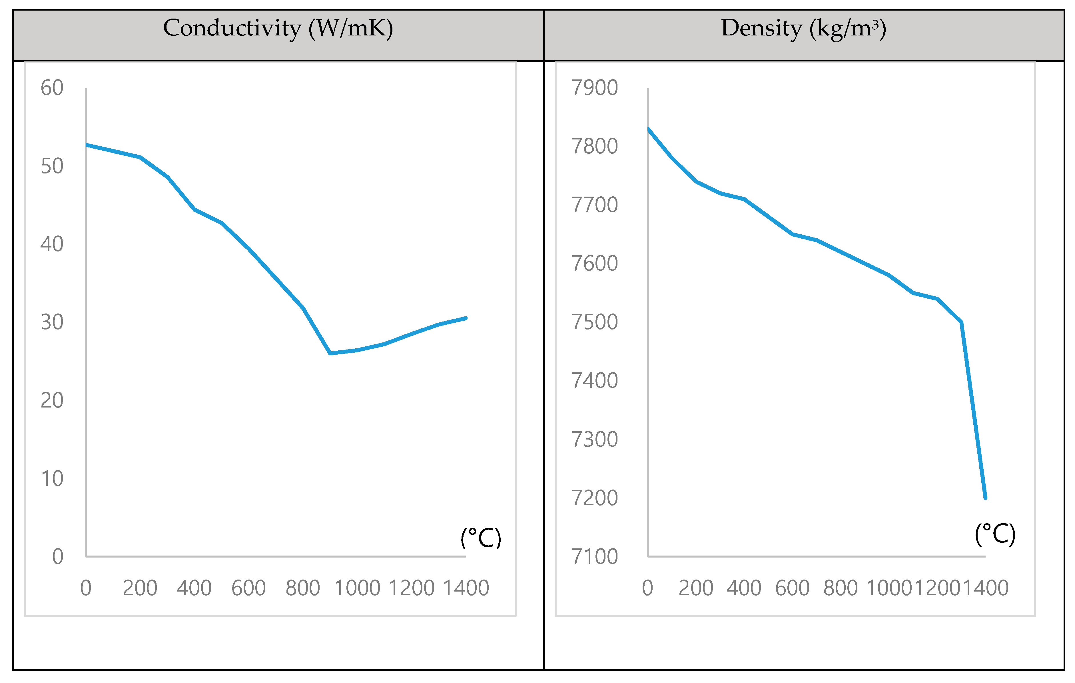
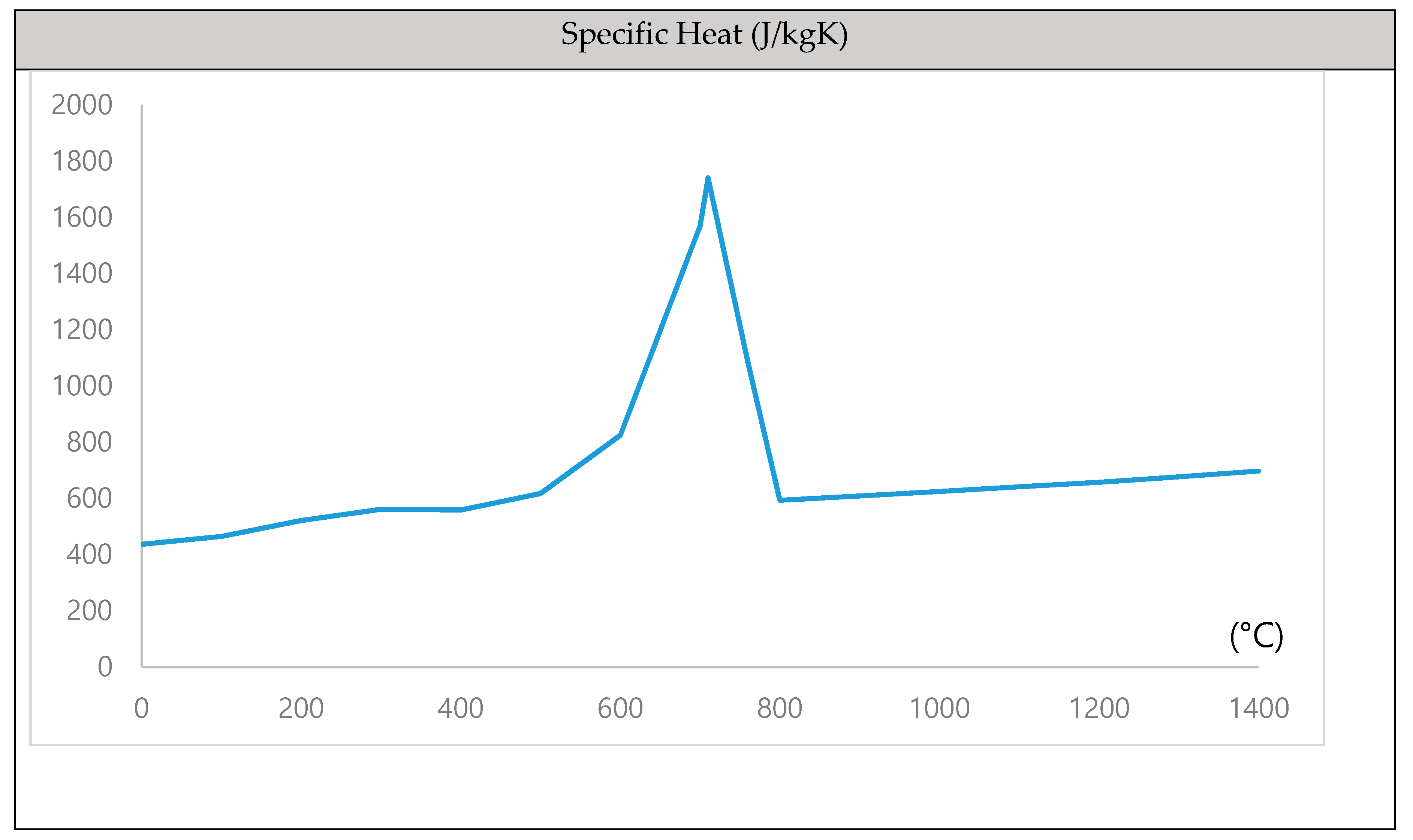
4.1. FE Simulation
4.2. Target and Variables
4.3. Algorithm Property
5. Results and Discussion
6. Conclusions
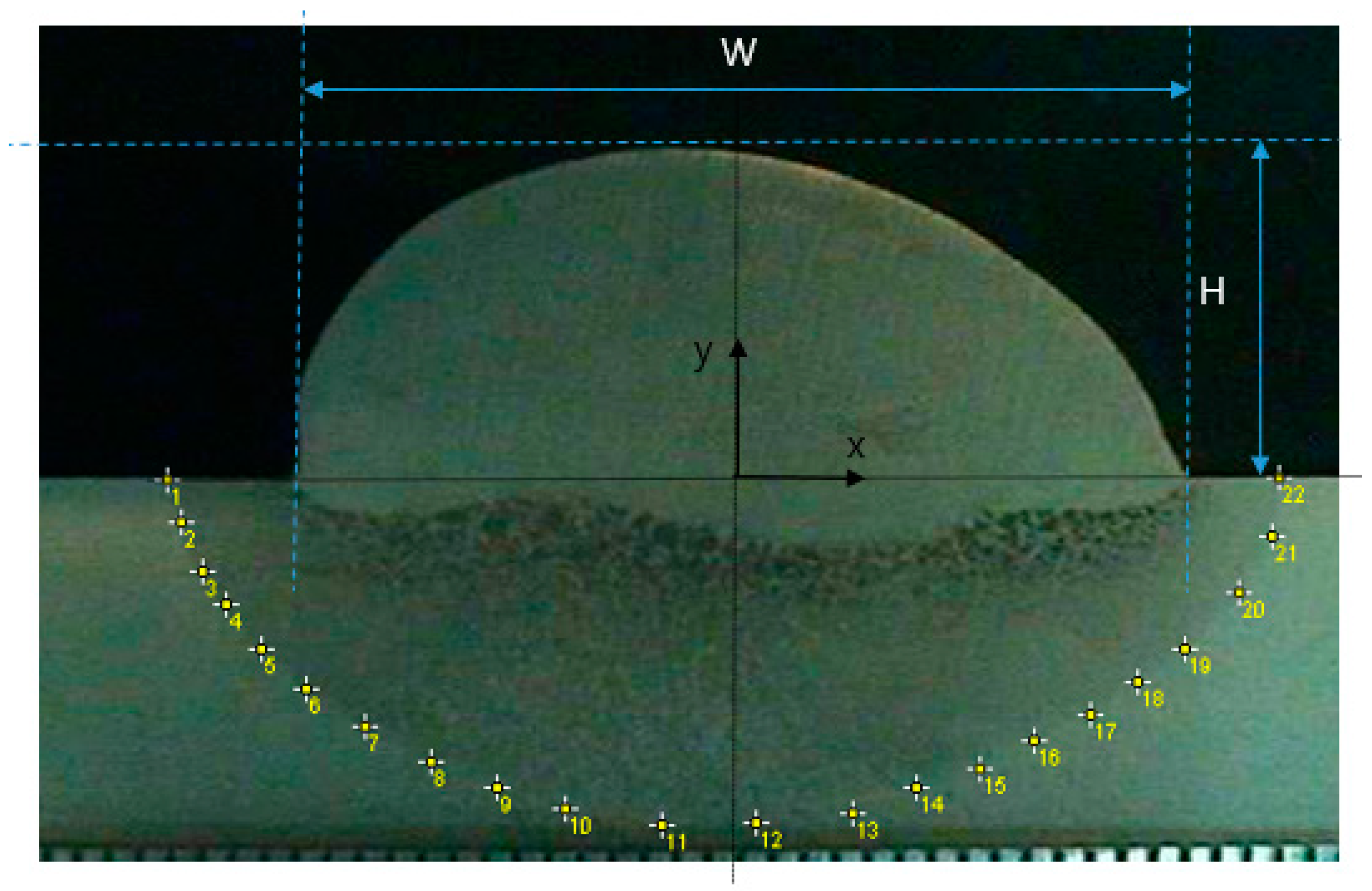
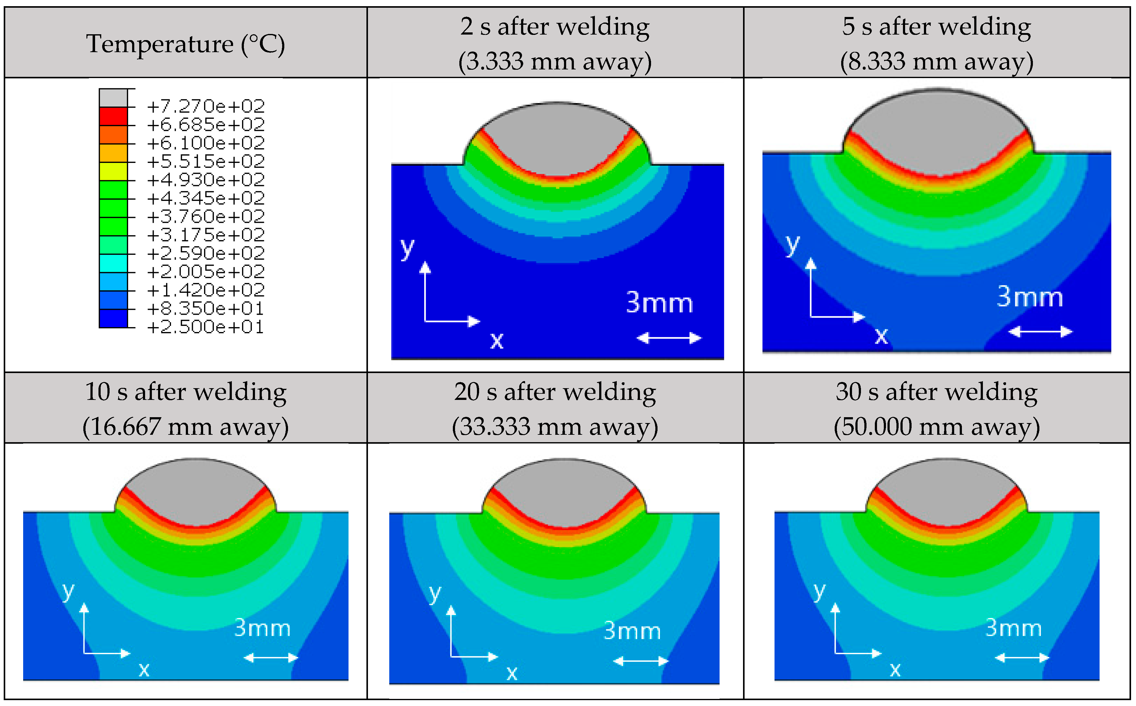
- The temperature distribution was confirmed by the finite element analysis using a moving heat source by simulating a BOP (Bead on Plate) test with SS400 plates.
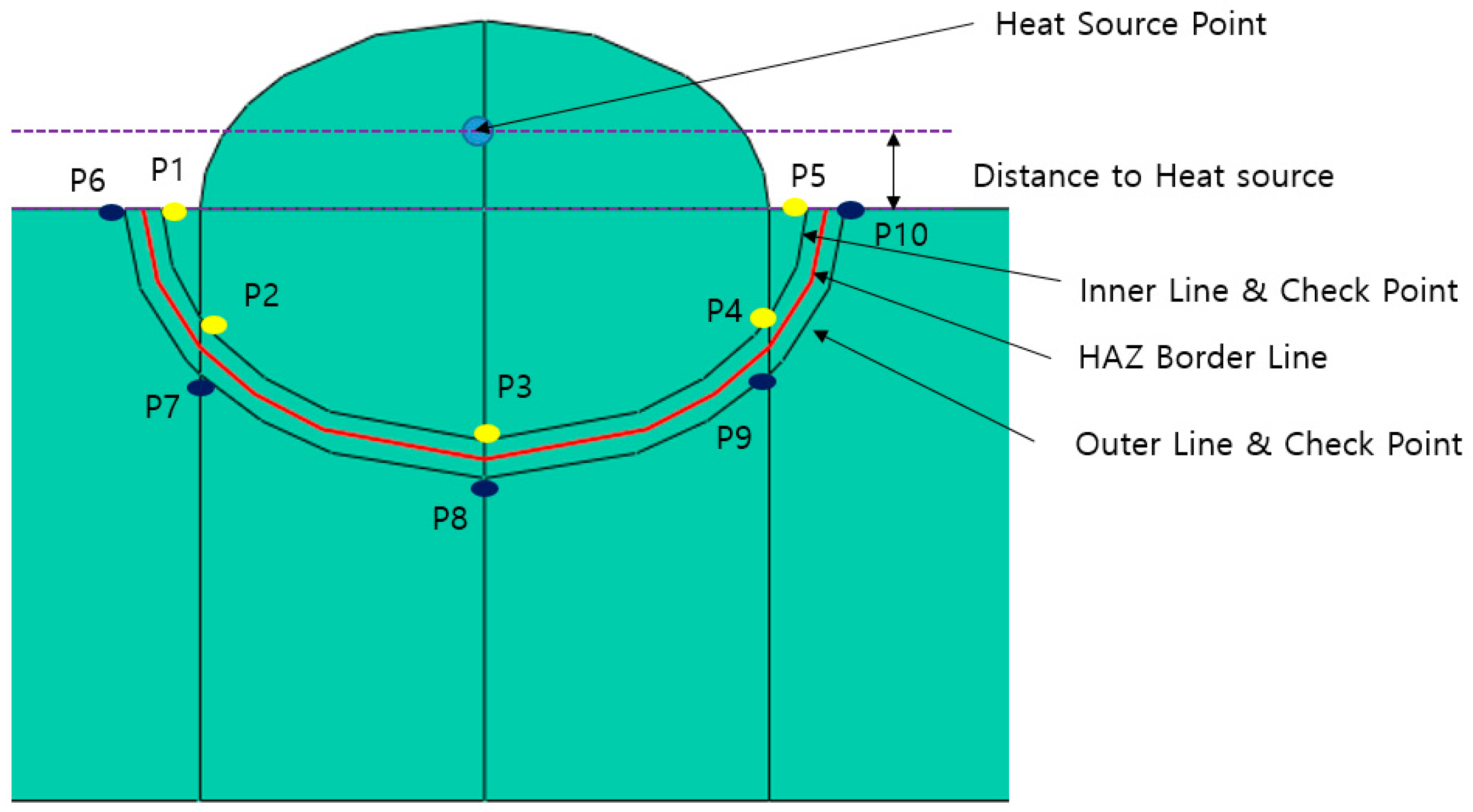
- The HAZ boundary of the specimen was coordinated, and the target was determined by analyzing the results at the line offset from the HAZ boundary. The target was set so that the temperature distribution of the inner offset line is 727 °C or higher and the outer offset line is 727 °C or lower.
- The optimal results were derived by using Isight’s multi-island algorithm. These results were derived by comparing over 1000 candidate groups by performing non-linear optimization using global optimization techniques.
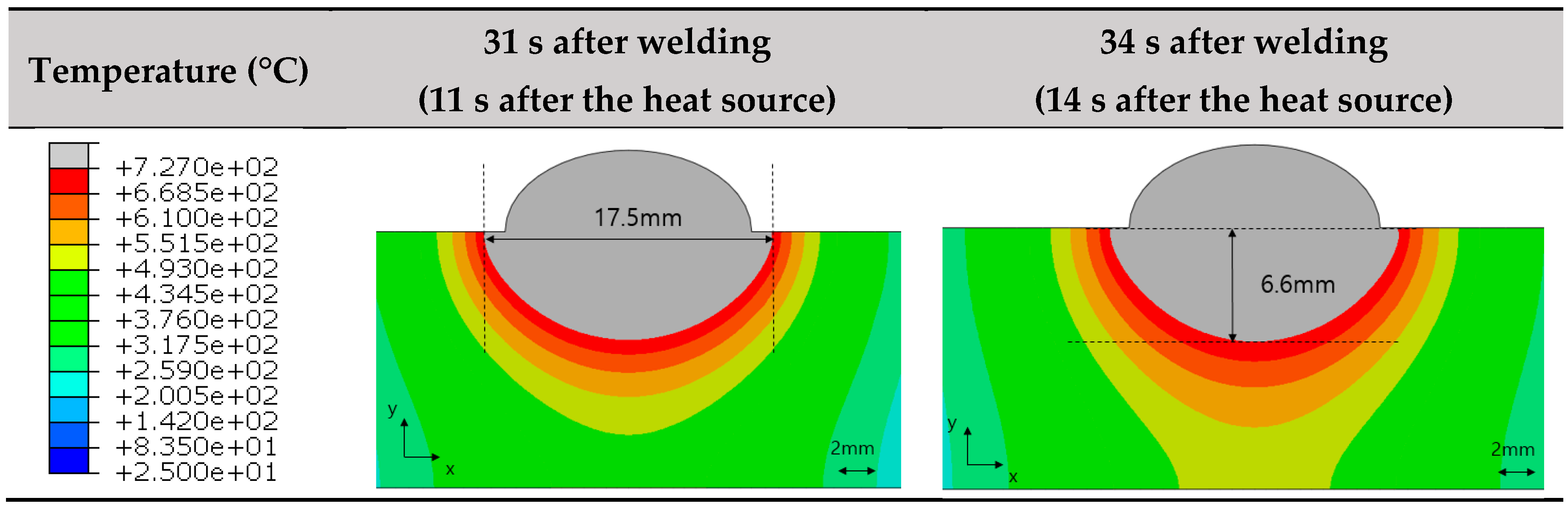
- Based on the results of global optimization, the HAZ boundary line was derived through finite element analysis, and was similar to the actual experimental results.
- Applying a search method using a multi-island algorithm was found to be useful in finding the welding heat source parameters required for welding heat transfer/thermal deformation analysis.
Author Contributions
Funding
Conflicts of Interest
References
- Jeshvaghani, R.; Harati, E.; Shamanian, M. Effects of surface alloying on microstructure and wear behavior of ductile iron surface-modified with a nickel-based alloy using shielded metal arc welding. Mater. Des. 2011, 32, 1531–1536. [Google Scholar] [CrossRef]
- Kannan, T.; Murugan, N. Effect of flux cored arc welding process parameters on duplex stainless steel clad quality. J. Mater. Process. Technol. 2006, 176, 230–239. [Google Scholar] [CrossRef]
- Gunaraj, V.; Murugan, N. Application of response surface methodology for predicting weld bead quality in submerged arc welding of pipes. J. Mater. Process. Technol. 1999, 88, 266–275. [Google Scholar] [CrossRef]
- Hu, J.; Tsai, H. Heat and mass transfer in gas metal arc welding. Part I: The arc. Int. J. Heat Mass Transf. 2007, 50, 833–846. [Google Scholar] [CrossRef]
- Sepe, R.; Armentani, E.; Lamanna, G.; Caputo, F. Evaluation by FEM of the influence of the reheating and post-heating treatments on residual stresses in welding. Key Eng. Mater. 2015, 627, 93–96. [Google Scholar] [CrossRef]
- Armentani, E.; Pozzi, A.; Sepe, R. Finite-element simulation of temperature fields and residual tresses in butt welded joints and comparison with experimental measurements. In Proceedings of the ASME 2014 12th Biennial Conference on Engineering Systems Design and Analysis, Copenhagen, Denmark, 25–27 June 2014. [Google Scholar]
- Armentani, E.; Esposito, R.; Sepe, R. The influence of thermal properties and preheating on residual stresses in welding. Int. J. Comput. Mater. Sci. Surf. Eng. 2007, 1, 146–162. [Google Scholar] [CrossRef]
- Rosenthal, D. The Theory of Moving Sources of Heat and Its Application to Metal Treatments. Trans. Am. Soc. Mech. Eng. 1946, 68, 849–866. [Google Scholar]
- Goldak, J.; Chakravarti, A.; Bibby, M. A new finite element model for welding heat sources. MTB 1984, 15, 299–305. [Google Scholar] [CrossRef]
- Lee, S.; Kim, E.; Park, J.; Choi, J. MIG Welding Optimization of Muffler Manufacture by Microstructural Change and Thermal Deformation Analysis. J. Weld. Join. 2017, 35, 29–37. [Google Scholar] [CrossRef] [Green Version]
- Tchoumi, T.; Peyraut, F.; Bolot, R. Influence of the welding speed on the distortion of thin stainless steel plates—Numerical and experimental investigations in the framework of the food industry machines. J. Mater. Process. Technol. 2016, 229, 216–229. [Google Scholar] [CrossRef]
- Chujutalli, J.H.; Lourenço, M.I.; Estefen, S.F. Experimental-based methodology for the double ellipsoidal heat source parameters in welding simulations. Mar. Syst. Ocean Technol. 2020, 15, 110–123. [Google Scholar] [CrossRef]
- Podder, D.; Mandal, N.R.; Das, S. Heat Source Modeling and Analysis of Submerged Arc Welding. Weld. J. 2014, 93, 183–192. [Google Scholar]
- Kim, J.W.; Jang, B.S.; Kim, Y.T.; Chun, K.S. A study on an efficient prediction of welding deformation for T-joint laser welding of sandwich panel PART I: Proposal of a heat source model. Int. J. Nav. Arch. Ocean. 2013, 5, 348–363. [Google Scholar] [CrossRef] [Green Version]
- Hu, X.; Chen, X.; Zhao, Y.; Yao, W. Optimization design of satellite separation systems based on Multi-Island Genetic Algorithm. Adv. Space Res. 2014, 53, 870–876. [Google Scholar] [CrossRef]
- Lin, B.; Yu, Q.; Li, Z.; Zhou, X. Research on parametric design method for energy efficiency of green building in architectural scheme phase. Front. Archit. Res. 2013, 2, 11–22. [Google Scholar] [CrossRef] [Green Version]
- Wang, Z.; Ma, J.; Zhang, L. State-of-Health Estimation for Lithium-Ion Batteries Based on the Multi-Island Genetic Algorithm and the Gaussian Process Regression. IEEE Access 2017, 5, 21286–21295. [Google Scholar] [CrossRef]
- Zhao, D.J.; Wang, Y.K.; Cao, W.W.; Zho, P. Optimization of Suction Control on an Airfoil Using Multi-island Genetic Algorithm. Procedia Eng. 2015, 99, 696–702. [Google Scholar] [CrossRef] [Green Version]
- Deng, D. FEM prediction of welding residual stress and distortion in carbon steel considering phase transformation effects. Mater. Des. 2009, 30, 359–366. [Google Scholar] [CrossRef]
- Narang, H.K.; Mahapatra, M.M.; Jha, P.K.; Sridhar, P.; Biswas, P. Experimental and Numerical Study on Effect of Weld Reinforcement on Angular Distortion of SAW Square Butt Welded Plates. J. Weld. Join. 2018, 36, 48–59. [Google Scholar] [CrossRef] [Green Version]
- Moradi, M.; Pasternak, H. A Study on the Influence of Various Welding Sequence Schemes on the Gain in Strength of Square Hollow Section Steel T-Joint. J. Weld. Join. 2017, 35, 41–50. [Google Scholar] [CrossRef] [Green Version]
- El-Sayed, M.; Shash, A.Y.; Rabou, M. Heat Transfer Simulation and Effect of Tool Pin Profile and Rotational Speed on Mechanical Properties of Friction Stir Welded AA5083-O. J. Weld. Join. 2017, 35, 35–43. [Google Scholar] [CrossRef]
- Wang, W.; Mo, R.; Zhang, Y. Multi-Objective Aerodynamic Optimization Design Method of Compressor Rotor Based on Isight. Procedia Eng. 2011, 15, 3699–3703. [Google Scholar] [CrossRef] [Green Version]
- Hahn, Y.; Cofer, J. Design Study of Dovetail Geometries of Turbine Blades Using Abaqus and Isight. In Proceedings of the ASME Turbo Expo 2012: Turbine Technical Conference and Exposition, Copenhagen, Denmark, 11–15 June 2012; Volume 7, pp. 11–20. [Google Scholar]
- Koch, P.; Evans, J.; Powell, D. Interdigitation for effective design space exploration using iSIGHT. Struct. Multidisc. Optim. 2002, 23, 111–126. [Google Scholar] [CrossRef]
- Layus, P.; Kah, P.; Khlusova, E.; Orlov, V. Study of the sensitivity of high-strength cold-resistant shipbuilding steels to thermal cycle of arc welding. Int. J. Mech. Mater. Eng. 2018, 13, 3. [Google Scholar] [CrossRef] [Green Version]
- Fu, G.; Lourenço, M.; Duan, M.; Estefen, S. Influence of the welding sequence on residual stress and distortion of fillet welded structures. Mar. Struct. 2016, 46, 30–55. [Google Scholar] [CrossRef]
- McKay, B. Evolutionary Algorithms. Encycl. Ecol. 2008, 1464–1472. [Google Scholar]
- Kim, J.; Kim, I.; Kim, Y. Optimization of weld pitch on overlay welding using mathematical method. Int. J. Precis. Eng. Manuf. 2014, 15, 1117–1124. [Google Scholar] [CrossRef]
- Pozo, L.P.; Olivares, F.; Durán, O. Optimization of welding parameters using a genetic algorithm: A robotic arm–assisted implementation for recovery of Pelton turbine blades. Adv. Mech. Eng. 2015, 7, 1687814015617669. [Google Scholar] [CrossRef] [Green Version]
- Gery, D.; Long, H.; Maropoulos, P. Effects of welding speed, energy input and heat source distribution on temperature variations in butt joint welding. J. Mater. Process. Technol. 2005, 167, 393–401. [Google Scholar] [CrossRef]
- Reda, R.; Magdy, M.; Rady, M. Ti–6Al–4V TIG Weld Analysis Using FEM Simulation and Experimental Characterization. Iran. J. Sci. Technol. Trans. Mech. Eng. 2019, 44, 765–782. [Google Scholar] [CrossRef]


| Type | Material | TS (MPa) | YS (MPa) | Elongation (%) | Hardness (HV) |
|---|---|---|---|---|---|
| Base metal | SS400 | 435 | 325 | 25 | 128 |
| Filler metal | AWS A5.29 | 550 | 470 | 19 | - |
| Material | Composition (%) | |||
|---|---|---|---|---|
| SS400 | C | Si | Mn | P |
| 0.15 | 0.05 | 0.697 | 0.113 | |
| S | Cu | Cr | Ni | |
| 0.007 | 0.041 | 0.087 | 0.503 | |
| AWS A5.29 | C | Si | Mn | P |
| 0.03 | 0.47 | 1.41 | 0.007 | |
| S | Cu | Cr | Ni | |
| 0.005 | - | 0.02 | 1.4 | |
| Parameter | Value | Parameter | Value |
|---|---|---|---|
| Current | 200 A | Shielding gas flow rate | 18 ℓ/min |
| Voltage | 24 V | Welding speed | 100 mm/min |
| Wire Feeding rate | 100 mm/min |
| HAZ Boundary | X-coordinate | Y-coordinate | HAZ Boundary | X-coordinate | Y-coordinate |
|---|---|---|---|---|---|
| Point 1 | −9.0 | 0.0 | Point 12 | 0.1 | −6.5 |
| Point 2 | −8.8 | −0.9 | Point 13 | 1.4 | −6.5 |
| Point 3 | −8.4 | −1.7 | Point 14 | 2.5 | −6.0 |
| Point 4 | −8.1 | −2.5 | Point 15 | 3.7 | −5.5 |
| Point 5 | −7.6 | −3.3 | Point 16 | 4.6 | −5.1 |
| Point 6 | −6.8 | −4.0 | Point 17 | 5.6 | −4.6 |
| Point 7 | −6.0 | −4.9 | Point 18 | 6.6 | −3.9 |
| Point 8 | −4.8 | −5.4 | Point 19 | 7.3 | −3.3 |
| Point 9 | −3.9 | −6.0 | Point 20 | 8.0 | −2.0 |
| Point 10 | −3.0 | −6.2 | Point 21 | 8.4 | −1.1 |
| Point 11 | −1.1 | −6.6 | Point 22 | 8.7 | −0.2 |
| Variables | Lower Bound | Upper Bound |
|---|---|---|
| af | 1.0 mm | 6.0 mm |
| ar/af | 2.0 | 7.0 |
| b | 1.0 mm | 10.0 mm |
| c | 1.0 mm | 8.0 mm |
| μ (weld efficiency) | 0.2 | 0.9 |
| Distance to heat source | 0 mm | 4.96 mm |
| Parameter | Value | Note |
|---|---|---|
| Sub-population size | 10 | Population by island |
| Number of islands | 10 | Number of islands |
| Number of generations | 10 | Total number of evolved generations |
| Rate of crossover | 100% | Crossover rate |
| Rate of mutation | 1% | Mutation rate |
| Rate of migration | 1% | Island migration rate |
| Interval of migration | 5 | Number of island migration generations |
| Candidate | μ | af | b | c | Distance to Heat Source (mm) | ar/af |
|---|---|---|---|---|---|---|
| 1 | 0.47 | 1.90 | 4.02 | 4.72 | 4.47 | 2.41 |
| 2 | 0.46 | 1.90 | 4.02 | 4.72 | 4.43 | 2.41 |
| 3 | 0.47 | 1.90 | 4.01 | 5.96 | 4.19 | 2.41 |
| 4 | 0.42 | 1.28 | 3.82 | 5.79 | 3.66 | 6.83 |
| 5 | 0.47 | 1.90 | 4.02 | 4.72 | 4.43 | 2.84 |
| 6 | 0.32 | 3.68 | 5.25 | 3.70 | 1.82 | 2.10 |
| 7 | 0.47 | 1.90 | 4.02 | 4.72 | 4.43 | 6.59 |
| 8 | 0.59 | 5.81 | 5.96 | 4.13 | 0.18 | 5.09 |
| 9 | 0.32 | 3.21 | 5.25 | 3.70 | 1.82 | 2.10 |
| 10 | 0.32 | 3.21 | 5.25 | 3.70 | 1.79 | 2.10 |
| Variables | Values |
|---|---|
| af | 1.9 mm |
| ar/af | 2.41 |
| b | 4.02 mm |
| c | 4.72 mm |
| μ (weld efficiency) | 0.47 |
| Distance to heat source | 4.47 mm (Bead height = 4.96 mm) |
| Dimension of HAZ | Experiment | Result of FEM |
|---|---|---|
| Width | 17.7 mm | 17.5 mm |
| Depth | 6.6 mm | 6.6 mm |
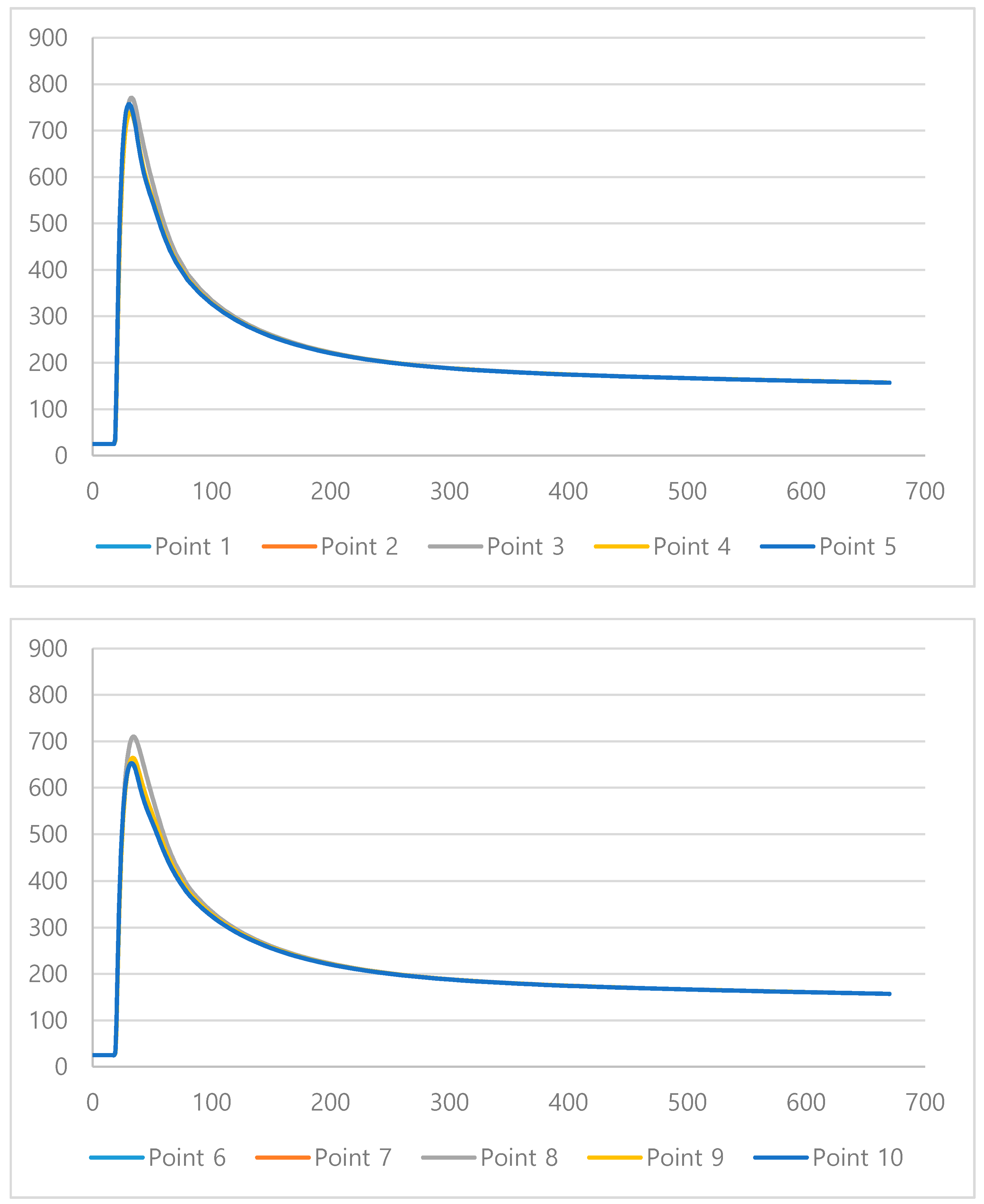
| Point | Value (°C) | Target value (°C) |
|---|---|---|
| Point 1 (P1) | 754.7 | >727 |
| Point 2 (P2) | 733.8 | >727 |
| Point 3 (P3) | 768.6 | >727 |
| Point 4 (P4) | 733.8 | >727 |
| Point 5 (P5) | 754.7 | >727 |
| Point 6 (P6) | 651.4 | <727 |
| Point 7 (P7) | 662.2 | <727 |
| Point 8 (P8) | 705.9 | <727 |
| Point 9 (P9) | 662.2 | <727 |
| Point 10 (P10) | 651.4 | <727 |
| Time(s) | P1 | P2 | P3 | P4 | P5 | P6 | P7 | P8 | P9 | P10 |
|---|---|---|---|---|---|---|---|---|---|---|
| … | ||||||||||
| 28 | 740.30 | 709.25 | 720.79 | 709.25 | 740.30 | 614.83 | 607.82 | 635.52 | 607.82 | 614.83 |
| 29 | 751.10 | 724.31 | 741.45 | 724.31 | 751.10 | 630.50 | 627.36 | 659.08 | 627.36 | 630.50 |
| 30 | 756.30 | 733.84 | 756.19 | 733.84 | 756.30 | 641.61 | 642.23 | 677.54 | 642.23 | 641.61 |
| 31 | 756.18 | 738.21 | 765.67 | 738.21 | 756.18 | 648.54 | 652.83 | 691.60 | 652.83 | 648.54 |
| 32 | 752.68 | 738.70 | 770.17 | 738.70 | 752.68 | 652.23 | 659.84 | 701.39 | 659.84 | 652.23 |
| 33 | 745.70 | 735.63 | 770.37 | 735.63 | 745.70 | 652.86 | 663.58 | 707.34 | 663.58 | 652.86 |
| 34 | 735.68 | 729.40 | 767.22 | 729.40 | 735.68 | 650.67 | 664.32 | 710.03 | 664.32 | 650.67 |
| 35 | 723.51 | 720.31 | 760.57 | 720.31 | 723.51 | 645.99 | 662.26 | 709.53 | 662.26 | 645.99 |
| 36 | 709.21 | 708.63 | 750.92 | 708.63 | 709.21 | 638.99 | 657.59 | 706.11 | 657.59 | 638.99 |
| 37 | 693.07 | 694.96 | 739.29 | 694.96 | 693.07 | 630.01 | 650.70 | 700.34 | 650.70 | 630.01 |
| 38 | 676.73 | 680.67 | 726.85 | 680.67 | 676.73 | 620.09 | 642.38 | 692.99 | 642.38 | 620.09 |
| … | ||||||||||
© 2020 by the authors. Licensee MDPI, Basel, Switzerland. This article is an open access article distributed under the terms and conditions of the Creative Commons Attribution (CC BY) license (http://creativecommons.org/licenses/by/4.0/).
Share and Cite
Pyo, C.; Kim, J.; Kim, J. Estimation of Heat Source Model’s Parameters for GMAW with Non-linear Global Optimization—Part I: Application of Multi-island Genetic Algorithm. Metals 2020, 10, 885. https://0-doi-org.brum.beds.ac.uk/10.3390/met10070885
Pyo C, Kim J, Kim J. Estimation of Heat Source Model’s Parameters for GMAW with Non-linear Global Optimization—Part I: Application of Multi-island Genetic Algorithm. Metals. 2020; 10(7):885. https://0-doi-org.brum.beds.ac.uk/10.3390/met10070885
Chicago/Turabian StylePyo, Changmin, Jisun Kim, and Jaewoong Kim. 2020. "Estimation of Heat Source Model’s Parameters for GMAW with Non-linear Global Optimization—Part I: Application of Multi-island Genetic Algorithm" Metals 10, no. 7: 885. https://0-doi-org.brum.beds.ac.uk/10.3390/met10070885