Article

Advanced Process Simulation of Low Pressure Die Cast A356 Aluminum Automotive Wheels—Part II Modeling Methodology and Validation

1
The Department of Materials Engineering, The University of British Columbia, 6350 Stores Road, Vancouver, BC V6T 1Z4, Canada
2
CITIC Dicastal Co., Ltd., No 185, Long Hai Road, Economic and Technological Development Zone, Qinhuangdao 066011, Hebei, China
*
Author to whom correspondence should be addressed.
Submission received: 2 September 2020 / Revised: 22 October 2020 / Accepted: 23 October 2020 / Published: 25 October 2020

Abstract

:
This manuscript presents an advanced modeling methodology developed to accurately simulate the temperature field evolution in the die and wheel in an industrial low-pressure die casting (LPDC) machine employed in the production of A356 automotive wheels. The model was developed in the commercial casting simulation platform ProCAST for a production die operating under production conditions. Key elements in the development of the model included the definition of the resistance to heat transfer across the die/casting interfaces and die/water-cooling channel interfaces. To examine the robustness of the modeling methodology, the model was applied to simulate production and non-production process conditions for a die cooled by a combination of water and air-cooling (Die-A), and to a second die for a different wheel geometry (Die-B) utilizing only water cooling for production conditions. In each case, the model predictions with respect to in-die and in-wheel temperature evolution were compared to industrially derived thermocouple (TC) data, and were found to be in good agreement. Once tuned to the process conditions for Die-A operating under production conditions, no further tuning of the die/casting interface resistance was applied. Additionally, the model results, in terms of the prediction of pockets of solid encapsulated liquid, were used to compare to x-ray images of wheels. This comparison indicated that the model was able to predict clusters of porosity associated with encapsulated liquid with an equivalent radius of ~27 mm.

1. Introduction

Low-pressure die casting (LPDC) is the primary process adopted to manufacture load-bearing aluminum automotive parts thanks to its ability to produce parts with a good balance of cost-effectiveness and performance [1,2,3,4]. It is a complex process that requires careful control of the filling and solidification stages in order to avoid the occurrence of defects that degrade component performance. Computer-based simulation, as a complement to experience, has become a crucial aspect in the development and optimization of both die-tooling and process operational parameters [5]. Driven by the increasingly strict requirements on weight, mechanical performance, geometric tolerance, microstructure and pore defects, increased emphasis is being placed on computer-based simulation as a means of achieving the necessary quality. In recognition of this, original equipment manufacturers (OEMs) have started requiring many of the wheel suppliers, including CITIC Dicastal, to demonstrate their ability to accurately simulate in-process wheel solidification as part of their supplier qualification processes.
In the past decade, the sophistication of simulations has reached a level whereat the key phenomena, including heat, mass and momentum transport occurring within the LPDC process, can be described. Despite this increased capability, few studies appear in the literature focused on commercial wheel production. Hetu et al. developed a coupled fluid flow-heat transfer model that was used to simulate the LPDC process for an automotive housing and a wheel [6]. Another example is the model developed by Merlin et al. for simulating the casting of A356 wheels [7]. Duan et al. developed a two-phase model to describe the fluid flow during the filling stage of wheel manufacturing and to predict the free surface-related defects, such as air entrainment [8]. In other studies, Fan et al. investigated macro-segregation and porosity formation with the aid of thermal–fluid compositional models [9,10].
However, the accuracy of these models is often limited due to insufficient understanding and descriptions of the complex physical phenomena that occur during the casting processes. Examples include the dynamics of the heat transport associated with (1) water cooling (which now dominates commercial production) [11,12], and (2) the interface between the die and casting (and to a lesser extent the interfaces between the different die components) [13,14]. The development of robust and accurate descriptions of boundary conditions describing these areas, and ultimately the overall accuracy of these models, has been undermined by the availability of high-quality, comprehensive data from the production line, which is technically challenging and expensive to acquire. For example, the studies conducted by Hetu et al. [6] and Merlin et al. [7] were not validated against quantitative in-process data—e.g., in-die and/or in-casting temperature data. One good example of work in which model results were compared to commercial data is the work done by Zhang et al. [15], which presents a complex numerical model developed in ABAQUSTM and its validation using the temperature data acquired from an LPDC process during the production of a conventional aluminum wheel. However, fluid flow at the filling stage was not modeled due to the limitations imposed by the software at the time of the investigation.
The trend in the casting industry of adopting a computational-based approach to mold design and process control requires highly accurate and robust models that can accurately explore design and process control options [16]. This manuscript presents an advanced modeling methodology developed for the industrial LPDC of automotive wheels. The modeling methodology presented in this manuscript has been developed and extensively validated using quantitative data measured from industrial production processes employing two die structures and three process conditions. A description of the instrumentation methodology and data measured for one of the two dies (Die-A) is presented in reference [17]—Part I of this study. The capabilities of the model for Die-A, operating under two different sets of process conditions (production and non-production), and for a second die with a different geometry (Die-B) operating under a third set of conditions (production), are presented in this manuscript by comparing the model results with the in-process derived data.

2. Model Development

The model was developed using the commercial software package ProCAST (A trademark of the ESI Group), which is one of the most commonly used packages in the industry for the simulation of casting processes.

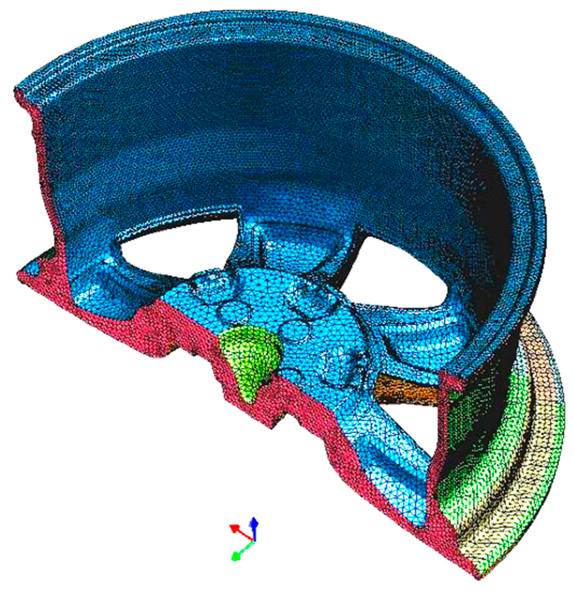
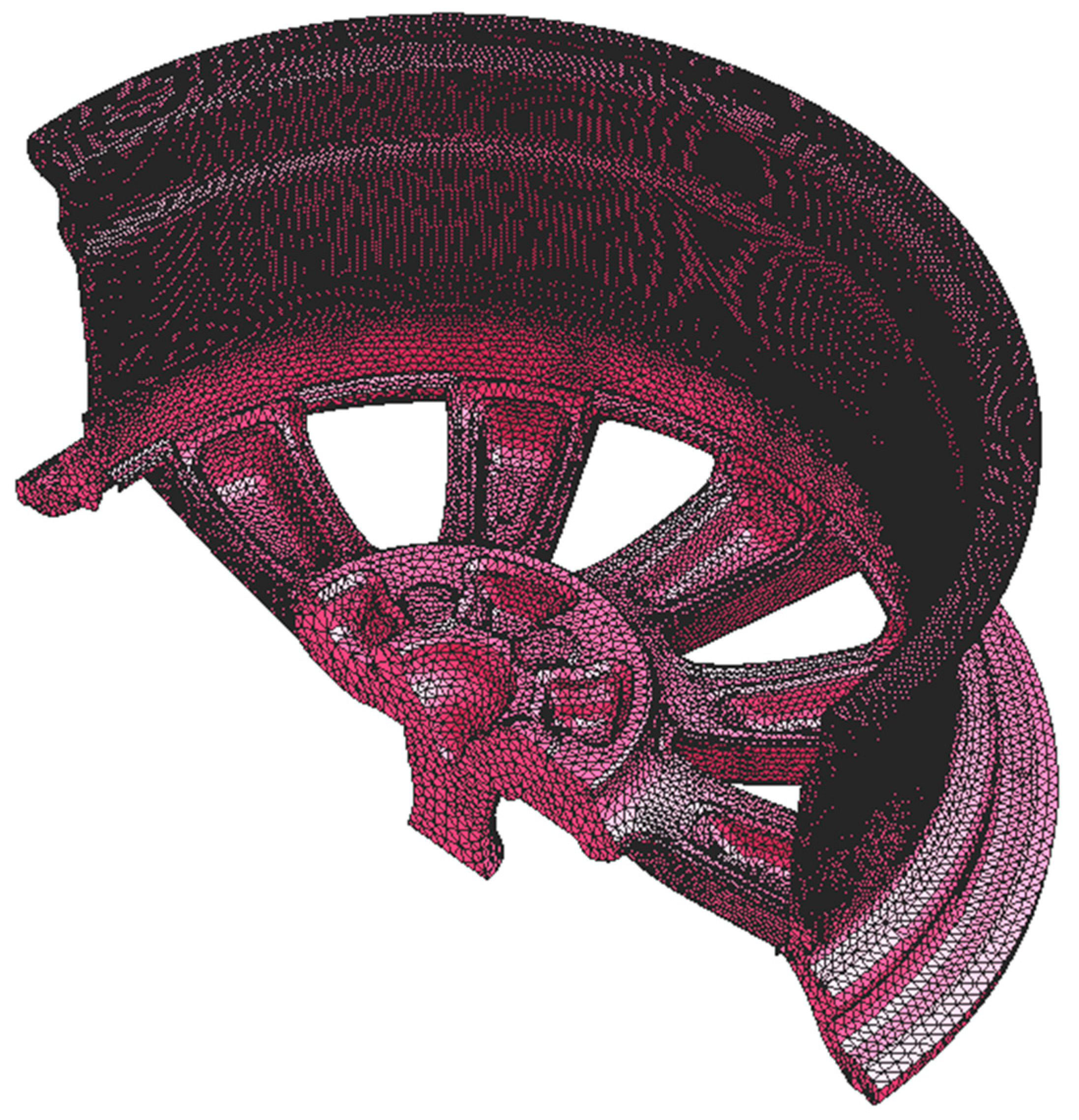
2.1. Geometry and Mesh

The components included in the computational domain are as follows: top die, side dies, bottom die and wheel. To reduce the computational size of the problem, the transfer tube and die support structures—e.g., top and bottom plates—were not included in the domain, since they are not expected to have a significant influence on the accuracy of the analysis. For the same reason, the venting features and ejection pins were also removed from the die structure. In addition, to take advantage of the mirror symmetry of the die and wheel structures, half of the die and wheel geometry has been used as the computational domain.
The strategy for meshing was to seek a balance between model accuracy and computational efficiency. In general, in regions that are relatively distant from the wheel and/or where a small temperature gradient is expected, a relatively coarse mesh was used. In contrast, in the wheel and regions where a high temperature gradient is expected, a fine mesh was employed. The following specific approaches were adopted:
  • In the rim of the wheel that has a relatively thin cross section, a 2 mm mesh size was selected to have at least 3–4 elements across the rim;
  • At the locations where strong heat transfer exists, i.e., in proximity to the cooling channels, a mesh size of 2 mm was selected;
  • A gradual increase of mesh size was implemented moving away from the wheel/die interface and cooling channels;
  • A default mesh size of 10 mm was used for the balance of the die geometry.
The resulting mesh for the wheel and die (Die-A) has 378,608 2D (surface) elements and 2,137,114 3D (body) elements (see the wheel mesh in Figure 1). The calculations were carried out on four processors of an Intel Xeon CPU (2.4 GHz). Computation time was approximately 1/2 h to run a single thermal-only analysis and 2 h to run a coupled thermal–fluid flow analysis.

2.2. Governing Equations

The governing equations describing energy, mass and momentum conservation in the computational domain are the classic Navier–Stokes Equations, which are given below:
ρ t + · ( ρ u ) = 0
ρ u t + · ( ρ u u ) = p + · τ + ρ g
ρ C P T t + · ( ρ C P T u ) = · ( k T ) + Q ˙
where ρ (kg/m3) is the density, t (s) is the time, u (m/s) is the velocity of the fluid, p (Pa) is the pressure, τ (Pa) is the shear stress, g (m/s2) is the gravitational acceleration, C P (J/(kg K)) is the specific heat at constant pressure, T (K) is the temperature, k (W/(m K)) is the thermal conductivity, and Q ˙ (J/(m3 s)) is the volumetric source term of heat, which incorporates the latent heat associated with the in-wheel solidification in this model. Note: the calculation of Q ˙ will be presented in Section 2.3.1.
The group of equations was solved subject to the specification of appropriate material properties, initial conditions and boundary conditions. Please note that the momentum conservation equation (Equation (2)) is only activated during the filling stage in ProCAST to save computation time. This means that the model assumes no fluid flow once the die cavity is fully filled and will no longer generate fluid flow-related results, i.e., fluid velocity. The modeling methodology was initially developed using the production process conditions for Die-A. This process involved some “tuning” of the internal and external interface conditions, which are described below in Section 2.5. The model is then applied to a second set of process conditions for Die-A (non-production) without retuning the model. The only changes to the model are related to the timing of activation and deactivation of the die cooling elements, and are applied in a consistent manner with the actual die machine process timings. Finally, the model is applied to a second die geometry, Die-B, with a third set of process timings (cooling element activation/deactivation and pressure fill curve), without retuning.

2.3. Materials and Properties
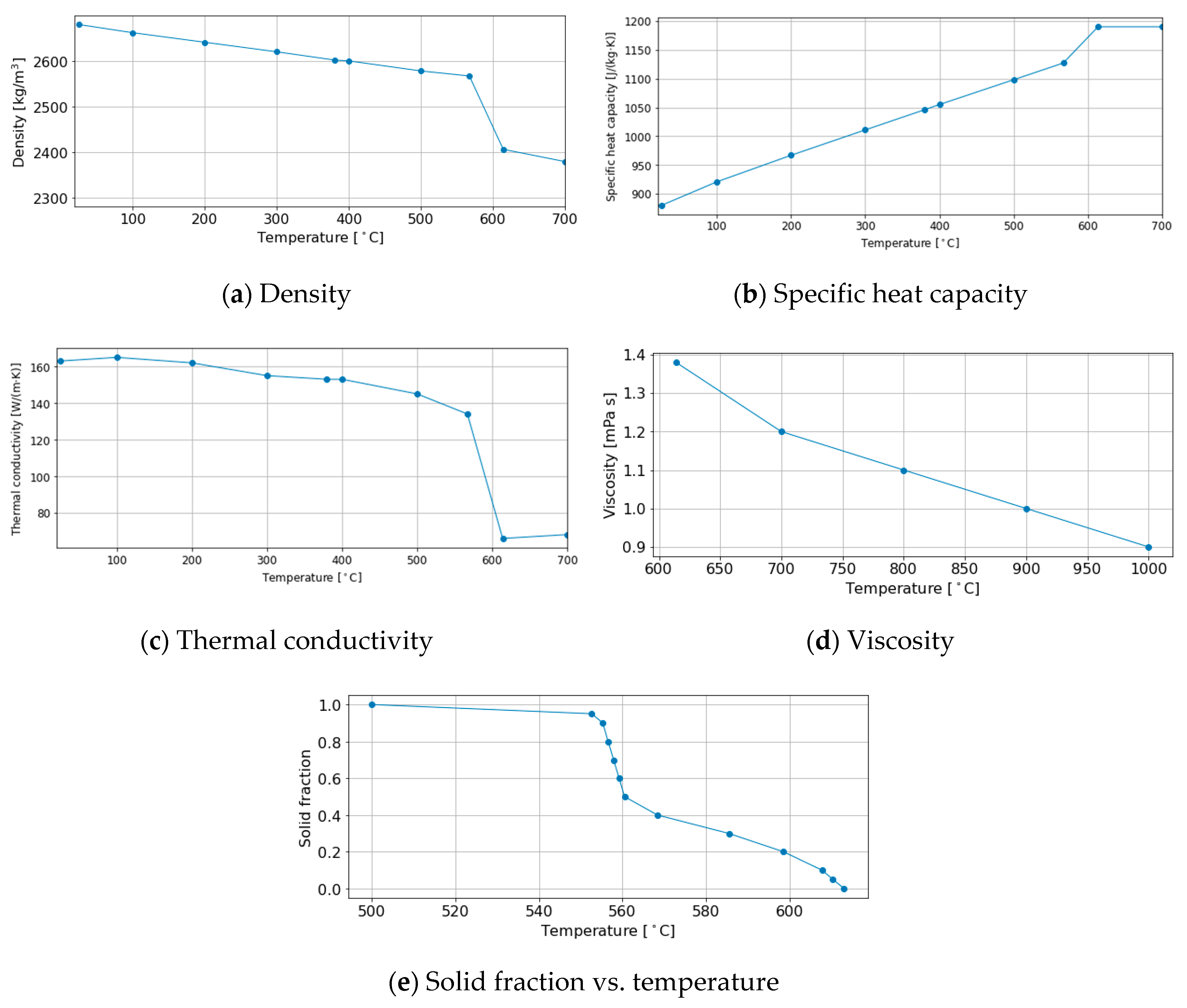
The materials used in the model are listed in Table 1, and their thermophysical properties are presented graphically in the following subsections. For those components that remain solid throughout the process—e.g., the die structure—only the properties required for solving the energy conservation equation are needed, which are density, thermal conductivity and specific heat. In contrast, the wheel material initially enters the die as a liquid, which then is transformed to a solid. Therefore, additional properties related to solving the momentum and continuity conservation equations, and dealing with the latent heat of solidification in the energy conservation equation, are needed for the wheel material A356. These include viscosity, solid fraction vs. temperature in the semi-solid region, and the latent heat of solidification.

2.3.1. A356 Wheel

The properties of the A356 used in the model are temperature-dependent and presented in Figure 2 [18,19]. Please note that, as indicated in Figure 2e, the solidus, eutectic transformation temperature and liquidus are 500 °C, 560 °C and 614 °C, respectively. Additionally, the latent heat associated with the in-wheel solidification (the heat source term, Q ˙ , in Equation (3)) is calculated by Equation (4).
Q ˙ = ρ L Δ f s Δ t = ρ L Δ f s Δ T Δ T Δ t
where   Q ˙ (J/(m3 s)) is the volumetric rate of heat release due to solidification, ρ (kg/m3) is the density, L (J/kg) is the specific latent heat (390 kJ/kg was used in the model), Δ f s Δ T (1/K) is the rate of change for the solid fraction with respect to temperature derived from Figure 2e, and Δ T Δ t (K/s) is the cooling rate at a given location calculated by the model.

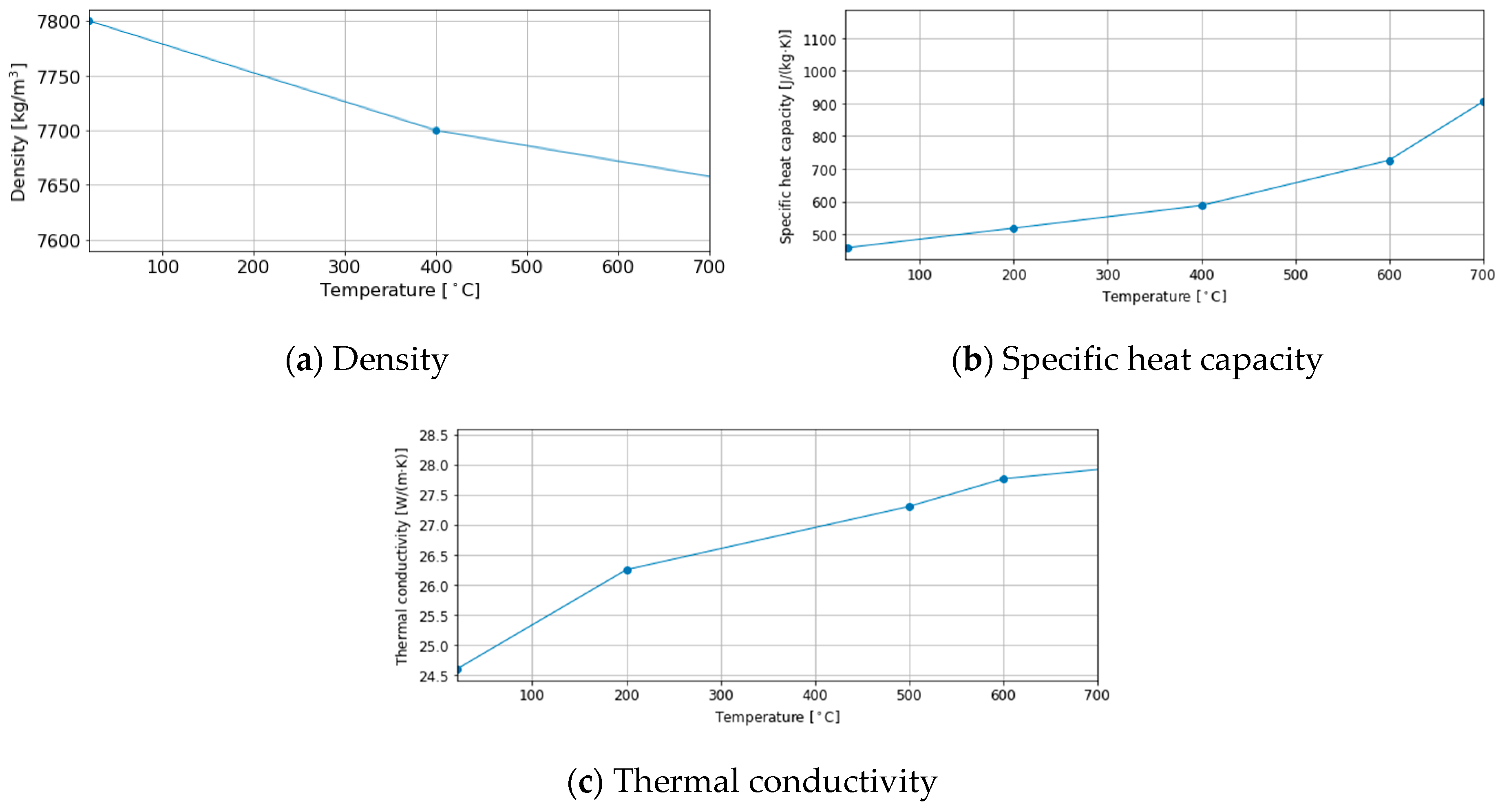
2.3.2. H13 Tool Steel—Top Die and Bottom Die

H13 tool steel is used for the top and bottom dies, and the properties are given in Figure 3 [15,18].

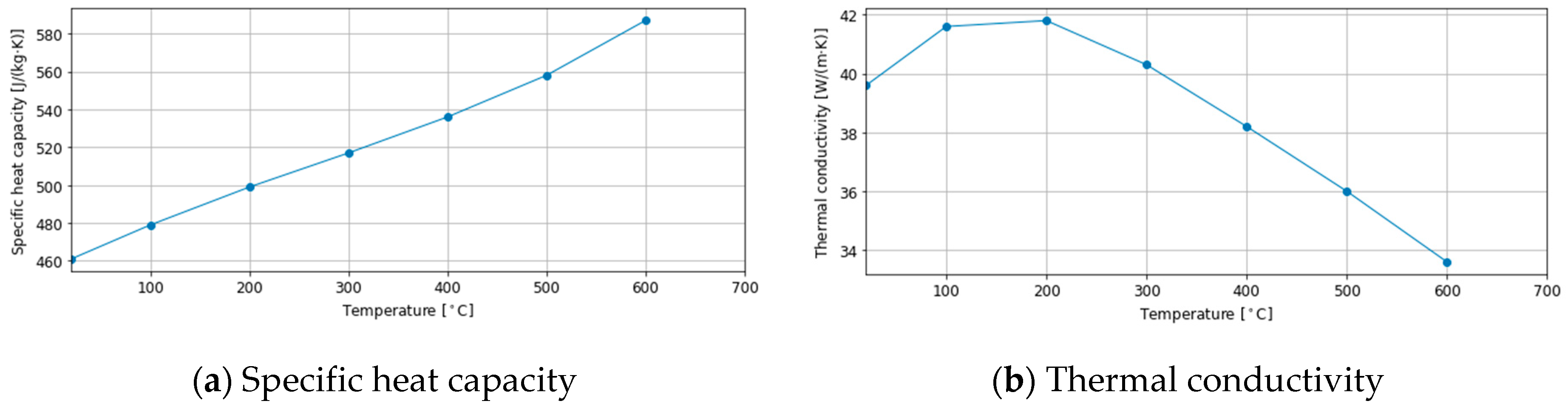
2.3.3. 35CrMo Tool Steel—Side Dies

The side dies are made from 35CrMo tool steel—the Chinese designation, which is equivalent to the German designation, 34CrMo4. The chemical compositions of both alloys are given in Table 2. It can be seen that the two alloys have negligible variation in composition, and therefore, the temperature-dependent thermal conductivity and specific heat capacity of 34CrMo4 are used in the model—see Figure 4, as those of 35CrMo are unavailable [20]. For the density, data in the appropriate temperature range is not available for both 34CrMo4 and 35CrMo. However, the density of alloys will not be significantly affected by small variations in the composition of alloying elements, and thus density data for H13 is used in the model. Note: Table 2 gives the composition of H13. The comparison of the densities of H13 and 34CrMo4 at room temperature only shows an ignorable difference—less than 1%.

2.4. Initial Conditions

In the commercial process, the die structure is typically pre-heated to between 300 and 500 °C using propane burners before the first casting cycle. However, due to the cyclic nature of the LPDC process, the die temperature will evolve over the first few casting cycles until eventually reaching the cyclic steady state for a given set of process conditions. The approach adopted in the present work is that the model is initially run for nine thermal-only cycles followed by six thermal and fluid flow cycles. For the initial thermal-only cycle, the die is set to 400 °C. In each subsequent cycle, the die structure is set to the temperature field calculated from the previous run. In the thermal only analyses, the calculation is executed with the die cavity full and at a uniform temperature of 700 °C at the beginning of each cycle. For the thermal–fluid flow analyses, the metal inlet temperature to the die is set to 700 °C and die filling is simulated together with the heat transfer during die filling. The approach described above greatly reduces the time required to achieve cyclic steady state as a thermal-only cycle takes ~25 min to run, whereas a coupled thermal and fluid flow cycle takes ~110 min. Cyclic steady state is assumed to have been achieved when the cycle-to-cycle thermal field in the die at the beginning of a cycle does not vary more than 5 °C.

2.5. Boundary Conditions

Since the model involves both heat transport and fluid flow, it requires the definition of two types of boundary conditions: (1) those associated with the thermal aspects of the analysis, and (2) those associated with the fluid flow aspects.

2.5.1. Thermal Boundary Conditions

All of the various thermal boundary conditions in this model are described using an equation of the form:
q = h ( T s u r f T r e f )
where q (W/m2) is the heat flux across the boundary, h (W/(m2 K)) is the heat transfer coefficient (HTC), and T s u r f (K) and T r e f (K) are the boundary surface temperature and the reference temperature, respectively. Note: the HTC represents the inverse of the resistance to heat transport across and at the interface between two solids or through a boundary layer between a solid and a fluid. There are two types of boundaries: one type is for interfaces where the boundary surface is internal and in contact with the surface of another component of the analysis domain, and the second type are interface is where the boundary is external and there is no contact with any other components. For the internal interfaces, the reference temperature, T r e f , in Equation (5) is the temperature of the adjacent surface in contact at the location being processed in the analysis, which varies with time and is calculated by the model. For the external surfaces, T r e f is set to the environment temperature, which is a user input. Please note that when the die is opened and the wheel is removed close to the end of a cycle, the casting/die interface is shifted from an internal type to an external type for the duration of the analysis of the cycle.
Heat Transport Across the Casting/Die Interfaces—The HTCs applied at the casting/die interfaces were determined through a combination of trial-and-error fitting to the production process data and experience, using the following principles:
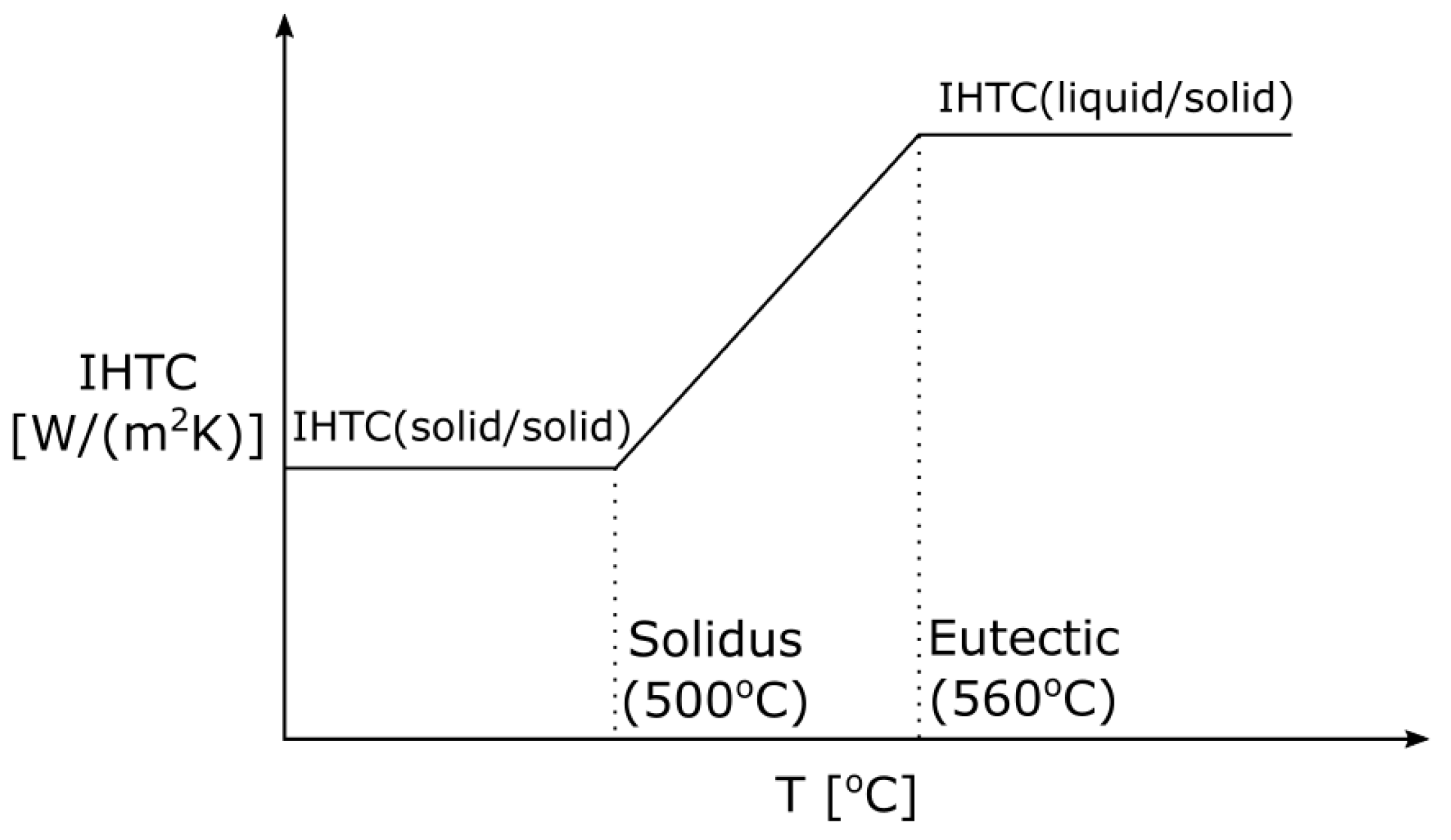
  • The HTCs applied at all casting/die interfaces are temperature-dependent, following the general behavior shown in Figure 5. When the temperature is above the eutectic transformation point of A356, and the metal is fully, or mainly, liquid, the HTCs are set to relatively high values since the liquid metal is in close-to-perfect contact with the die. In contrast, when the temperature is below the solidus and the wheel is fully solidified, the contact degrades, resulting in lower values of HTCs due to the formation of solid/solid interfaces. Depending on the interface location, it is possible for a gap to form between the casting and the die surface, which leads to lower HTC values. In the region between the eutectic transformation point and solidus, the HTCs are assumed to vary linearly.
  • Values of the HTCs for the different casting/die interfaces are given in Table 3. For the casting/bottom die interface, the HTC for the liquid/solid regime of behavior is higher compared to the other two interfaces. The rationale is that the bottom die has geometrically complicated features resulting in more complex flow during die filling, and therefore enhanced heat transfer. On the other hand, for the casting/top die interface, the HTC for the solid/solid regime of behavior is the highest as the wheel contracts onto the top die, placing the interface under pressure, and minimizing the development of resistance associated with gap formation.
As previously described, the casting/die interface changes from an internal interface to an external interface once the die is opened and the wheel is ejected. Correspondingly, these boundaries will be in contact with environmental air, and an HTC of 20 W/(m2 K) is used together with a reference temperature of 50 °C—see Equation (5).
Heat Transport Across the Die/Die Interfaces—The die/die internal interfaces are solid/solid interfaces throughout the process, and therefore, the HTCs of these interfaces are assumed to be invariant with temperature. Table 4 gives the HTCs used for the die/die interfaces. The values are again determined by a combination of trial-and-error and experience. Generally, the HTCs are high, and reflective of close contact following die assembly and closure of the die components. Similar to the casting/die interfaces, when the various die component interfaces lose contact due to die operations (e.g., separations), then 20 W/(m2 K) is used for the HTC and 50 °C for the reference temperature.
Water Cooling—Heat transfer associated with the water cooling in the cooling channels is one of the most important, but most complicated and dynamic, phenomena occurring during the LPDC process. Production-derived data indicates that boiling of the cooling water occurs at both the water-on and -off stages—refer to Part I of this study [17]. To incorporate boiling and its effect on heat transfer, the method described by Moayedinia [11] is used to calculate the cooling channel HTCs. An example of the relationship used in the model is presented in Figure 6. When the temperature is relatively low, no boiling occurs, and heat is extracted by forced convection. The HTC varies in a range between 4200 and 5000 W/(m2 K), dependent on the flow rate, diameter of the channel and temperature-dependent properties of the water. At interface temperatures above ~120 °C, the water in the cooling channels at the interface starts to boil. Note: the channel pressure is >1 atm. These bubbles agitate the boundary layer between the fluid and die, resulting in enhanced heat transfer—i.e., increases in the HTC. Peak heat transfer is predicted to occur at approximately ~160 °C. Above ~160 °C, interface contact gradually becomes reduced due to the formation and expansion of large vapor bubbles at the interface, and the HTC drops. Above ~240 °C, the HTC is assumed to be constant at 5000 W/(m2K). The reference temperature for the water-cooling boundary conditions, T r e f , is set to 50 °C, which is based on the average temperature change measured in the cooling water.
In addition, as indicated by the in-channel temperature and pressure data, boiling routinely occurs after the cooling water is switched off [17]. Note that, in the commercial process, even though the channels are purged with air for 10 s, there is still a certain amount of residual water left in the cooling channels, which then begins to boil, extracting significant amounts of heat from the die. The amount of water in a given channel was found to be dependent on the location of the channel in the die and the arrangement of the supply/drain lines affixed to the die. In the model, to represent the heat extracted by the post-water-off boiling, a constant heat flux of −1.5 × 10⁵ W/m2 is applied to the channels during the water-off periods. It is acknowledged that using a constant heat flux is a simplified approach. However, this approach was necessary to overcome limitations in the version of the software used in the study—i.e., only one temperature- and time-dependent HTC can be applied per cooling channel.
Air Cooling—Forced air cooling was employed at a number of locations in the dies studied in this work. In the model, an HTC of 200 W/(m2 K) and reference temperature of 50 °C are used at the locations where air cooling was applied.
Heat Transfer to Environment—Heat transfer on the outer surfaces of the die to the surrounding plant environment can occur through convection and radiation. The convective heat transfer is described in Equation (5), while the radiative transport has been described using the Stefan–Boltzmann equation—Equation (6). The parameters related to the environmental heat transfer are given in Table 5.
q r a d = ε σ ( T s u r f 4 T e n v 4 )
where q r a d (W/m2) is the heat flux by radiation, ε is the emissivity and σ (W/(m2 K4)) is the Stefan–Boltzmann constant.

2.5.2. Fluid Flow Boundary Conditions

Pressure Inlet—In the actual process, the flow rate of liquid into the die is controlled via the pressure in the holding furnace. In the model, the flow is controlled by the pressure applied at the inlet of the die cavity (sprue). The pressure applied in the model is a modified form of the machine-specified pressure curve following Equation (7), since the transfer tube is excluded from the computational domain.
P m o d e l = P m a c h i n e ρ A 356 g h t u b e
where P m o d e l (Pa) is the pressure used in the model and P m a c h i n e (Pa) is the process-specified pressure variation with time programmed into the die casting machine. ρ A 356 (kg/m3) is the density of A356, g (m/s2) is the gravitational acceleration and h t u b e (m) is the height of the space between the sprue and liquid metal surface in the holding furnace. The term ρ A 356 g h t u b e represents the pressure required to raise the liquid metal in the transfer tube to the sprue.

2.5.3. Time Steps

The model starts with an initial time step of 0.001 s. Subject to solution convergence, the time step is automatically adjusted but limited to the maximum time steps of 0.1 and 1 s for the filling stage (solution of fluid flow is activated) and the solidification stage (thermal only), respectively. Note: a sensitivity analysis was conducted with these parameters to assess their impact on the model results vs. execution time. These parameters were selected because they offer a balance between computational accuracy and efficiency.

3. Results and Discussion

Part I of this work reported on the method used for the process characterization of Die-A for two process conditions, and presented and discussed a representative selection of the data obtained—see reference [17]. The model validations for the two process conditions for Die-A are presented in Section 3.1, Section 3.2 and Section 3.3, followed by a comparison of the model predictions with a selection of data obtained from the production process for Die-B (Section 3.4).

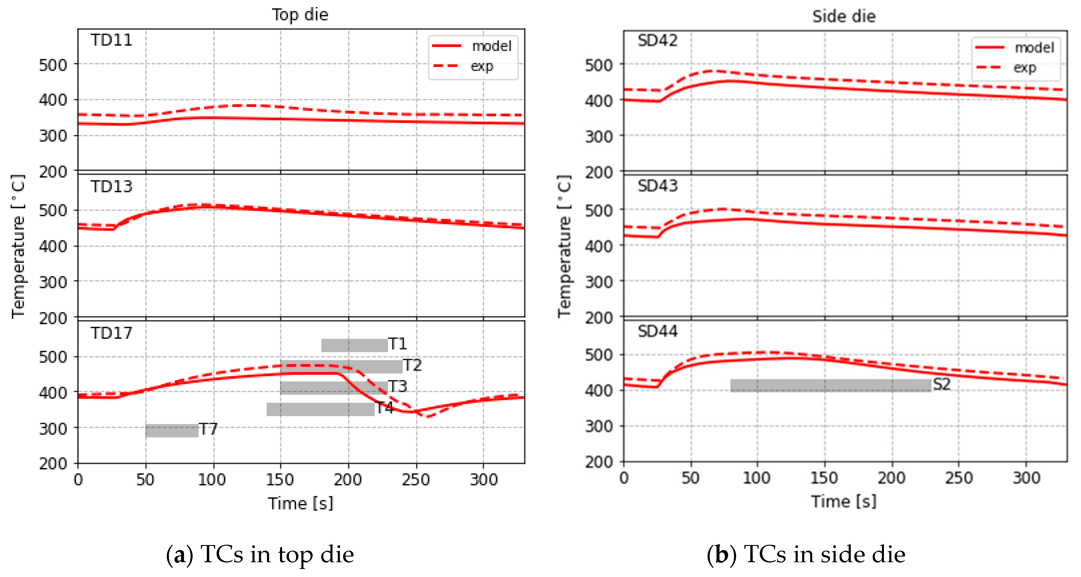
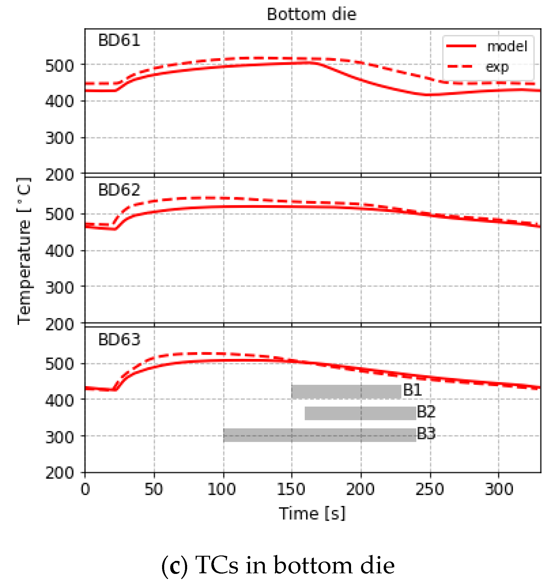
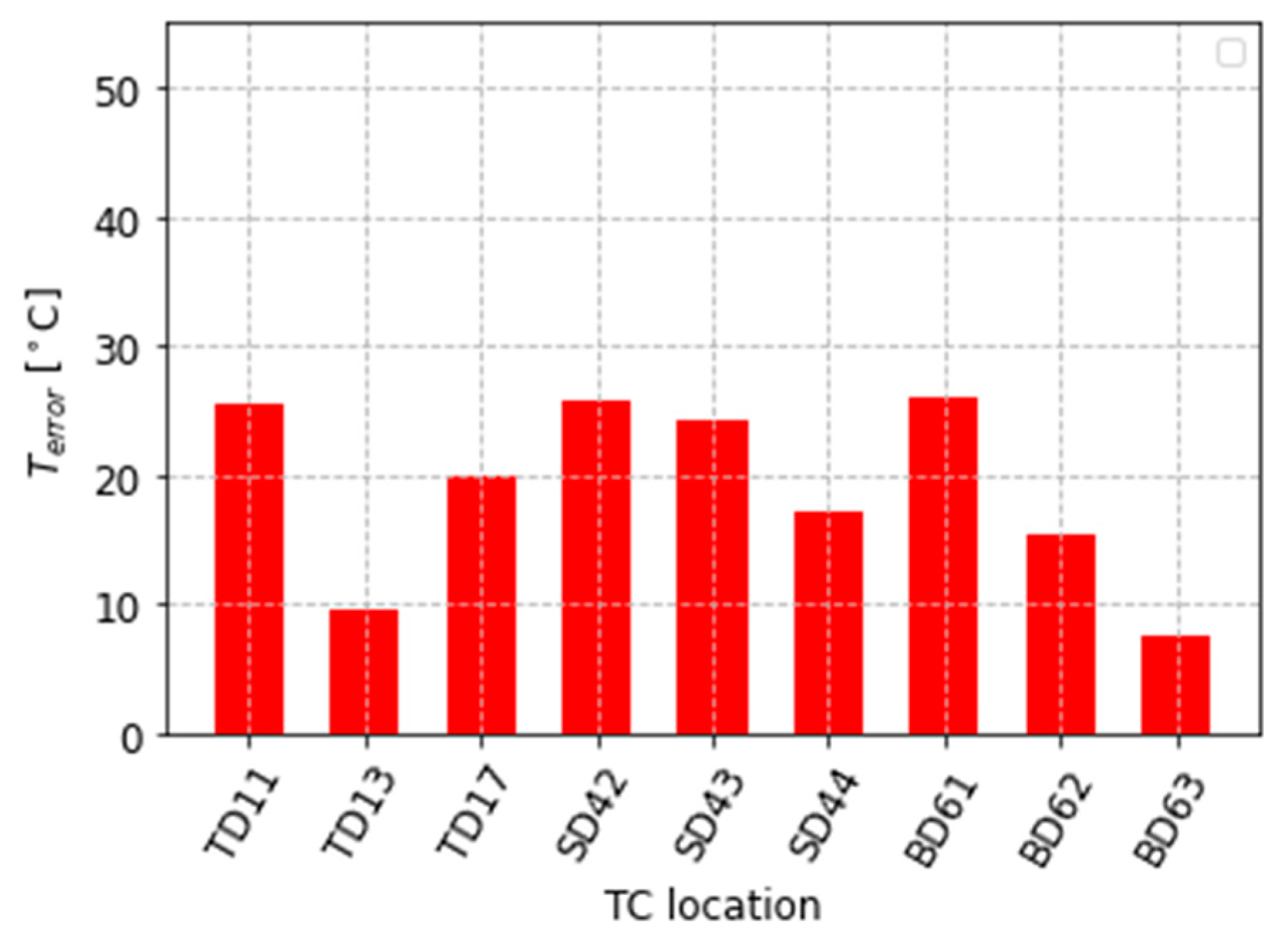
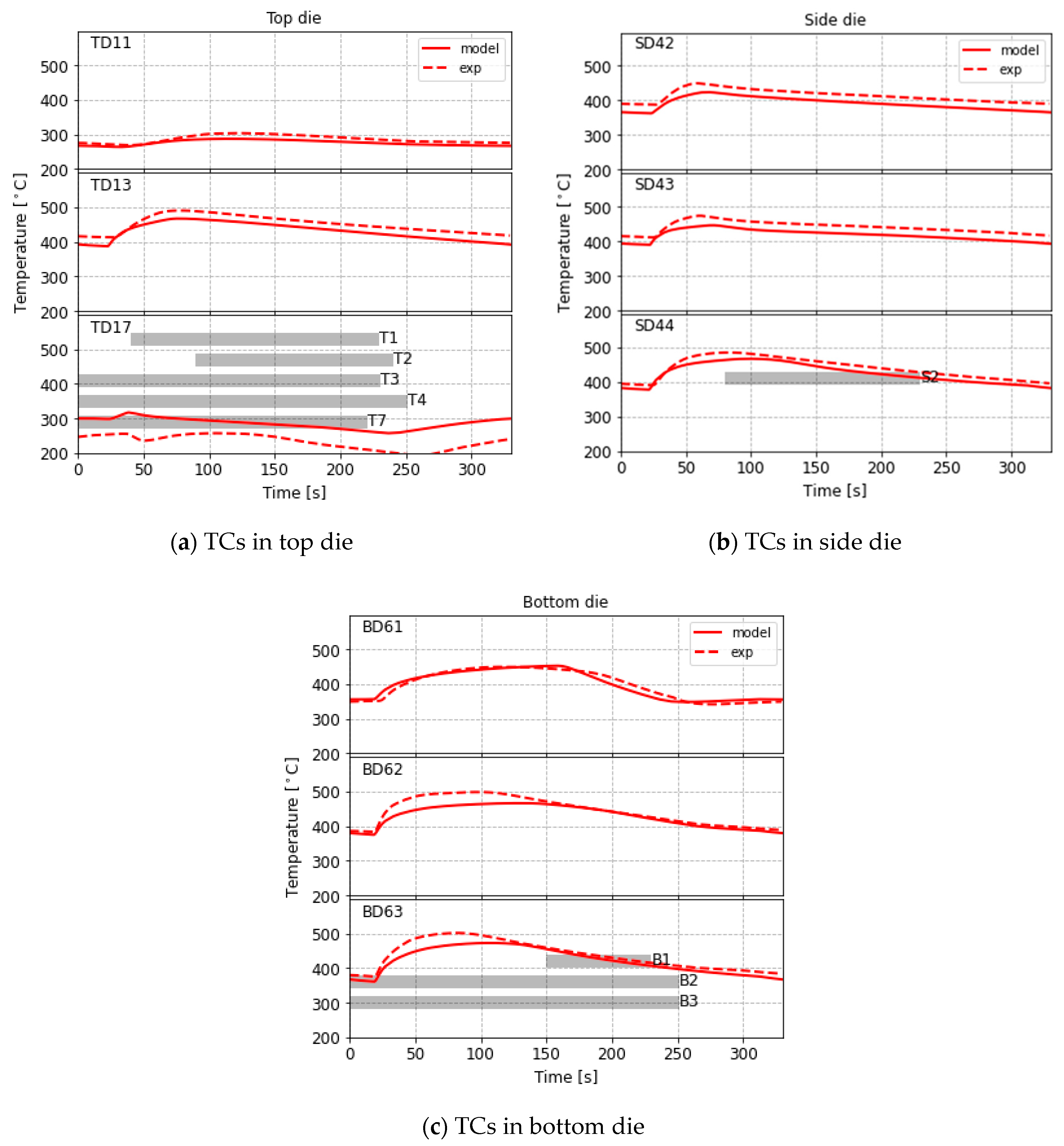
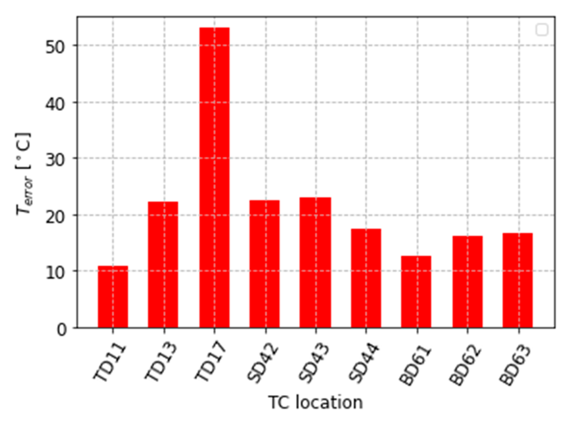
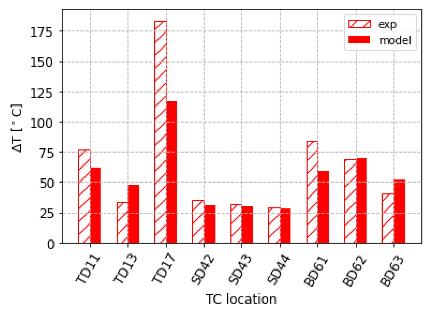
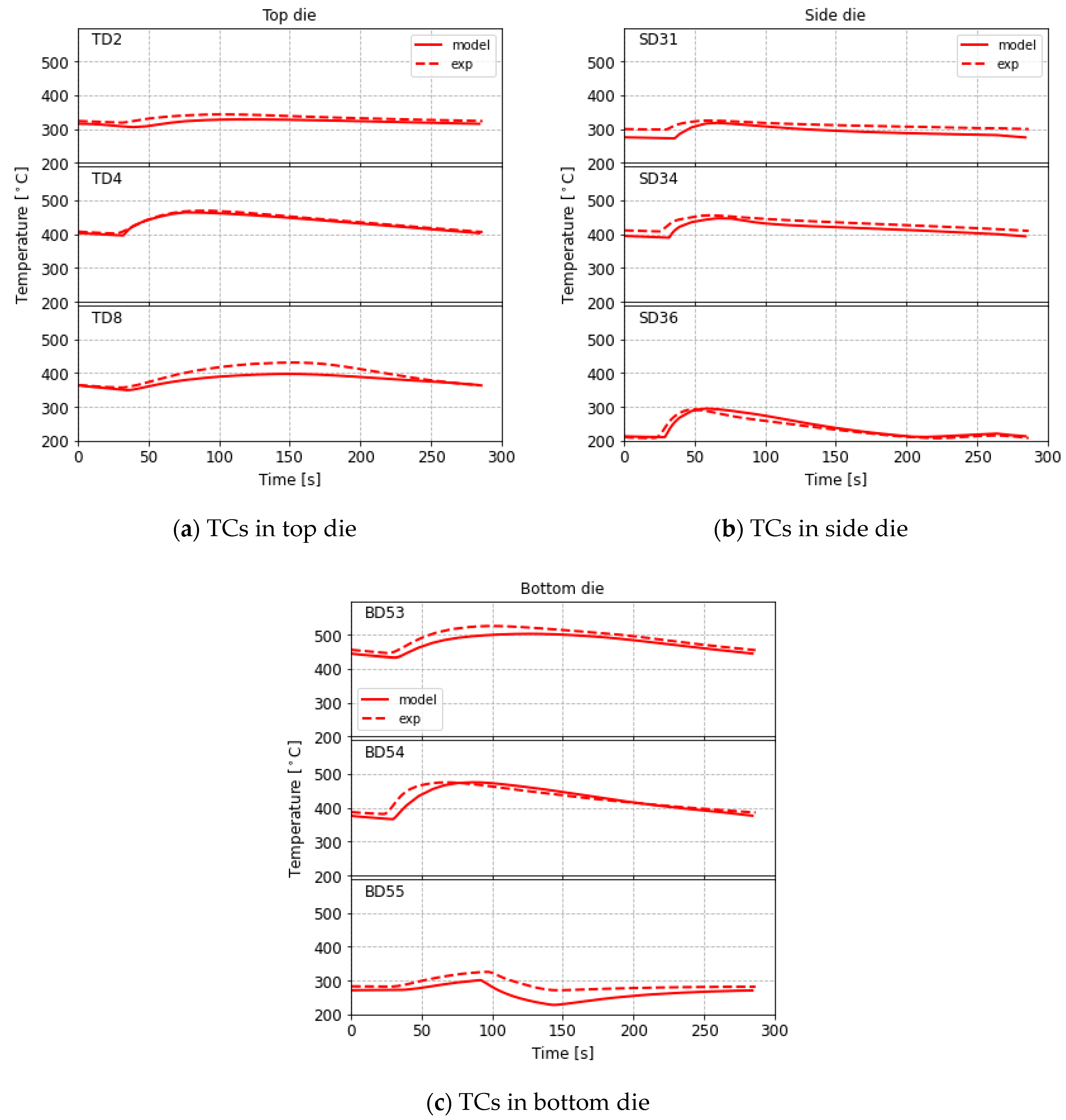
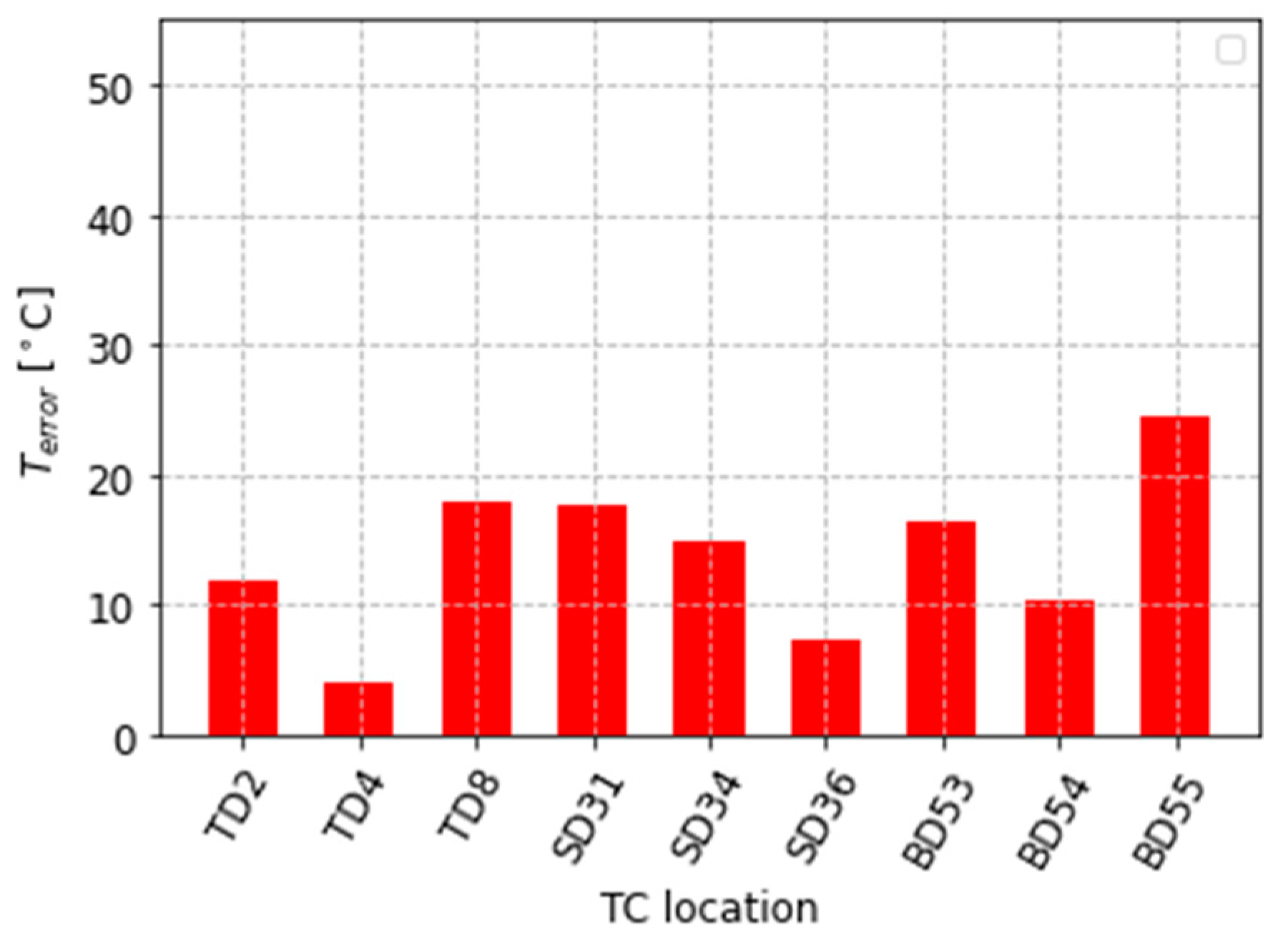
3.1. In-Die Temperature

The location of the nine in-die TCs used for model verification are shown in Figure 7a. Each die component has three TCs, which are distributed widely—see BD61, 62 and 63, SD44, 43 and 42, and TD11, 13 and 17. Figure 7a also shows the location of the cooling elements in each of the die components of Die-A—see B1, 2, 3, 5, S2, and T1, 2, 3, 4, 5, 7. B1, B5, S2, T1, T3, T5 and T7 are all water-cooling channels/elements. The remainder are air-cooling elements. The approach to die design is to have a generic number of elements, some of which are then activated for a given wheel geometry, thus providing flexibility in process control.
Production Process Condition—For the production process condition, Figure 8a–c present the in-die temperature comparison between the model and measured data at the TC locations in the top, side and bottom dies, respectively. Note: the cooling timings of the active cooling elements in each die component are also illustrated in the figures by the grey bars. In addition, the averaged error between the modeled and measured temperature data has been calculated by Equation (8) and displayed in Figure 9.
T e r r o r =   i = 1 N a b s ( T i ,   m o d e l T i ,   e x p ) N
where T e r r o r (K) is the error in temperature between the model, T i ,   m o d e l (K), and experimental measurements, T i ,   e x p (K), at time index i, and N is a large number (300), representing the number of sub-increments the casting cycle time has been divided into.
Overall, it can be seen that the model agrees very well with the measured data at all the locations in each die component with respect to both the magnitude and variation of temperature with time. The error ( T e r r o r ) is in the range of 6 to 27 °C. More specifically, the model is capable of capturing all three stages in the temperature evolution at all of the locations. The three stages and phenomena that give rise to them are discussed in detail in Part I of this work [17]. Briefly:
  • Stage-1 is characterized by a small drop in temperature until such time as the pulse of heat associated with the presence of liquid metal in the die cavity is able to diffuse through the die to the TC location;
  • Stage-2 is characterized by a rise in temperature associated with the transfer of heat from the aluminum into the die;
  • Stage-3 is characterized by a period of slow decline in die temperature associated with the balance between removal of heat from the die and the supply of heat from the solidifying wheel.
A closer look at the comparison shows that relatively large discrepancies appear at two locations, TD17 and BD61, and are both approximately 50 °C in magnitude at their maximum. They also both occur only in the third stage of the temperature evolution. As the third stage, characterized by cooling, is dependent on the activation of water-cooling elements, it is therefore speculated that the boundary conditions in the model describing the water cooling are responsible. Firstly, the effect of boiling has been included; however, its description is still simplified, and secondly, there is a delay between the time when the cooling water valve opens and when the water actually arrives at the in-die channels—see the details in Sections 4.1.2 and 4.1.4 of reference [17]. However, considering that one major aim of this work is to standardize the model parameters for extensive industrial use, and given that the delay varies from channel-to-channel, the cooling timings in the model were not adjusted relative to the programmable logic controller (PLC) set values to improve the fitting.
Non-Production Process Condition—In the non-production process condition, the cooling parameters were adjusted while the rest of the process parameters and boundary conditions were kept identical to the production process condition for Die-A. Figure 10a–c present the in-die temperature comparison at the selected TC locations in the top, side and bottom dies, respectively. Additionally, the error in temperature between model and measured data is presented in Figure 11. In general, at most locations (except for TD17), the model results match closely to the measured data ( T e r r o r < 23 °C). This demonstrates that the modeling approach is able to accurately capture a broad range of process cooling timings.
To assess the extent to which the changes in the process conditions (production vs. non-production) have changed the die temperature field at the steady state, and also the ability of the model to capture this change, the average change in temperature ∆Tavg has been calculated for the top, bottom and side TC locations according to the expression given in Equation (9).
Δ T a v g =   i = 1 N Δ T i N
where ∆Ti (K) is the difference in temperature between the production and non-production temperatures at time index i and N is a large number (300), representing the number of sub-increments the casting cycle time has been divided into. This has been done for both the TC data and for the model output at the TC locations. The results are presented in Figure 12 and indicate that the temperature difference between the two process conditions examined ranges from 30 to 90 °C, for most of the TC locations. At these locations, the differences based on the model predictions are in relatively good agreement. At TD17, however, a much larger average temperature difference in the process data is observed (~ 185 °C), whereas the model predicts this difference to be ~120 °C—a mismatch of approximately 65 °C. This mismatch is large and warrants a closer look.
TD17 was located very close to the water-cooling channel T3, which was instrumented with a TC (TD21)—refer to reference [17] Section 4.1.4 for the details related to the instrumentation of water-cooling channels. The results for TD21 for the production and non-production process conditions are presented in Figure 13a,b, respectively. Note: the water-on and air-purging periods are marked by the light purple and green bars, respectively, in the two figures. The major difference between these two sets of data is that, in the production process condition, the residual water remaining after air purging is fully vaporized and the channel dries out (after ~280 s). The “dry out” is indicated by the rise in temperature to well in excess of 100 °C, which continues through into the next casting cycle until the water-cooling is reactivated, whereas in the non-production process, the residual water in channel T3 is not fully vaporized (the temperature within the cooling channel remains just below 100 °C). Thus, the extended cooling time applied to channel T3 has had a secondary effect, in that by cooling the die to a larger extent, residual water is retained in the channel. Consequently, the period over which boiling occurs during the water-off period for the channel is extended from ~40 to ~90 s, leading to the large ∆Tavg observed in Figure 12. This effect is not currently captured within the model, hence the model under-predicts the effect of extending the cooling timing in channel T3. It also points to the need to fully understand the cooling/boiling behavior in the water channel during and after air purging.

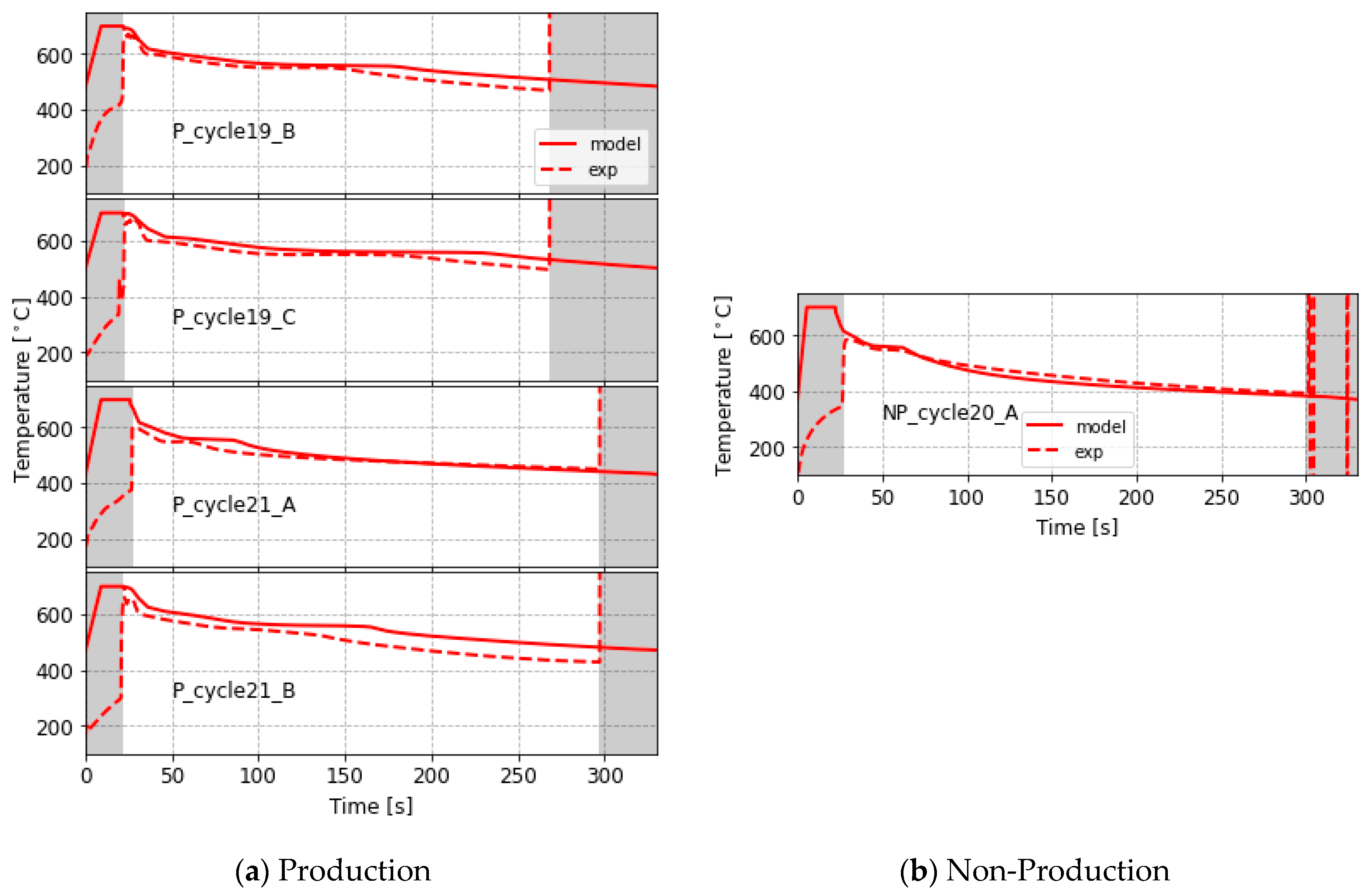
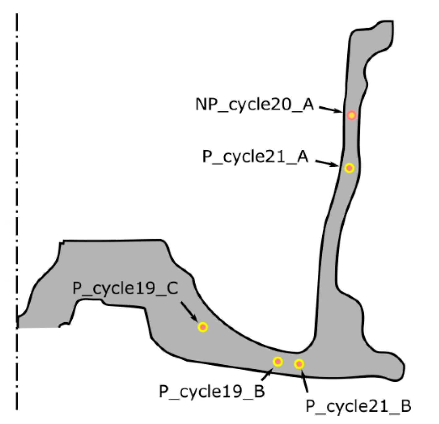
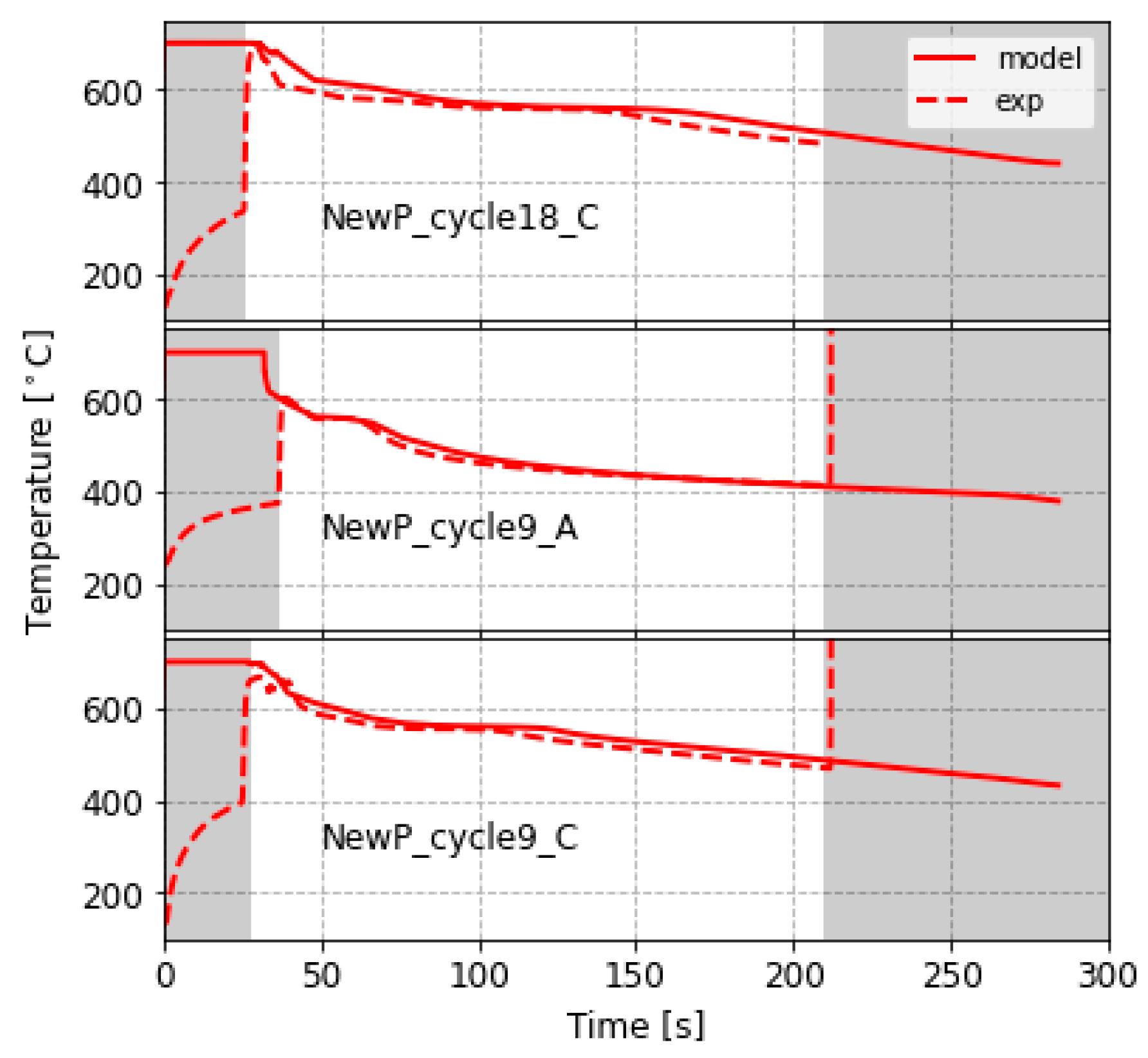
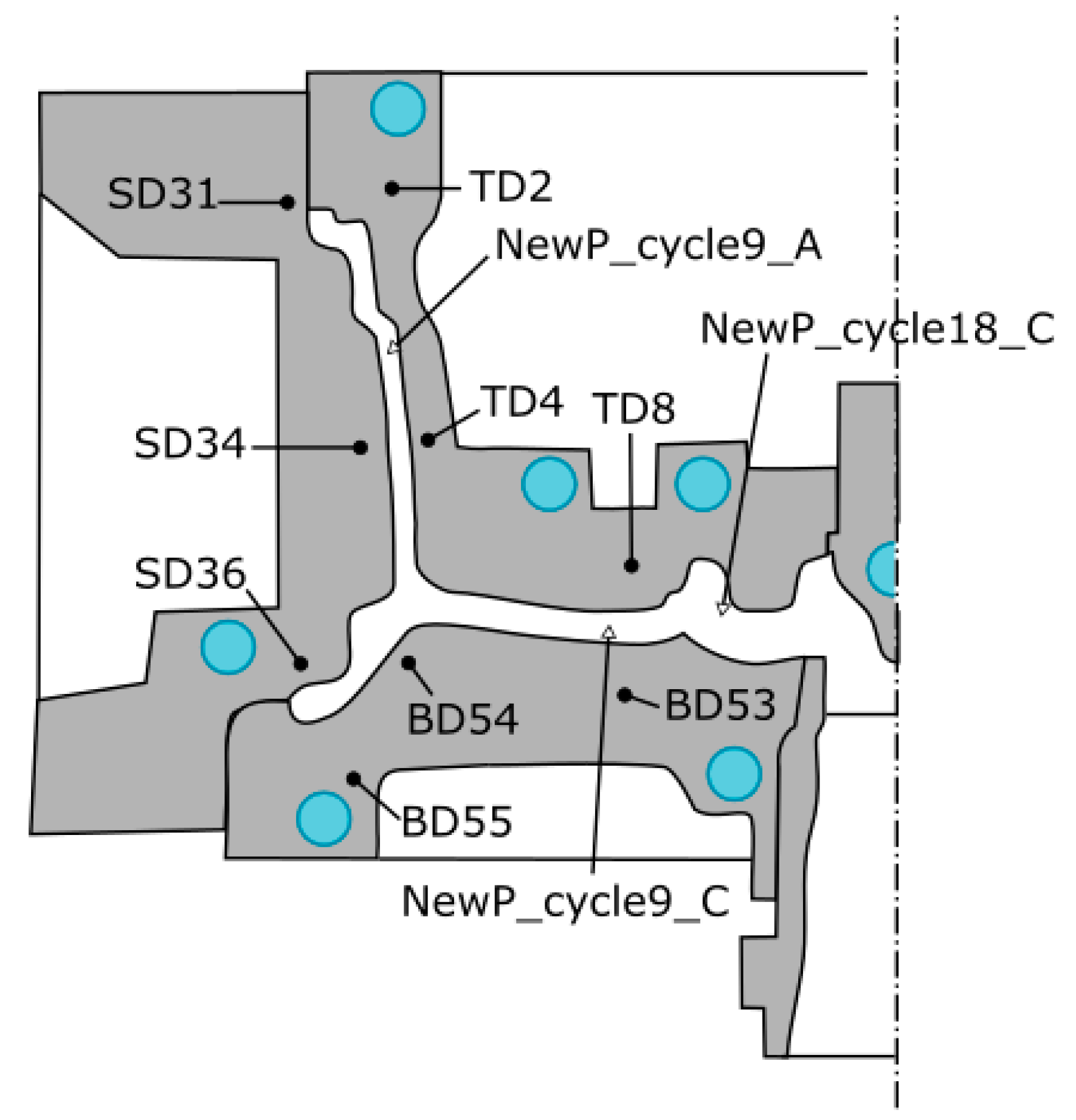
3.2. In-Wheel Temperature

The temperature evolution with time within the wheel at multiple locations was also examined in this work, which provides an opportunity for a direct validation of the model with respect to the thermal phenomena occurring during the solidification process. Figure 14a,b present a comparison between the in-wheel temperature measurements and the model predictions for the production and non-production process conditions, respectively. The in-wheel TC locations are shown in Figure 15. Those locations labeled with a P are for the production process condition and those labeled with an NP are for the non-production process condition. Note that there was only one successful insertion of a TC into the die cavity for the non-production process condition. It should be mentioned that these are challenging measurements to make, and that the TCs have to be inserted by hand into the die cavity and are prone to be cut when the die closes. There are two periods of time in which the data from the TCs should be disregarded: the first is at the beginning of the cycle prior to the liquid contacting the TC, and the second is at the end of the cycle when the TC is cut prior to the ejection of the wheel from the top die. In the figures, these periods are highlighted in light gray for clarity.
From the comparison, it can be seen that, overall, the model-predicted in-wheel temperatures follow the profiles of the measured data relatively well. The poorest agreement is observed for locations P_cycle21B and P_cycle19B, both of which are located in the spoke near the rim–spoke junction. In P_cycle21B, the error is approximately 50 °C at the end of the cycle. As can be seen, the model and experimental data both reflect the latent heat release associated with primary α-aluminum solidification at approximately ~600 °C and eutectic formation at ~560 °C, as evidenced by periods of reduced rates in temperature decline—see reference for solidification sequence [19].

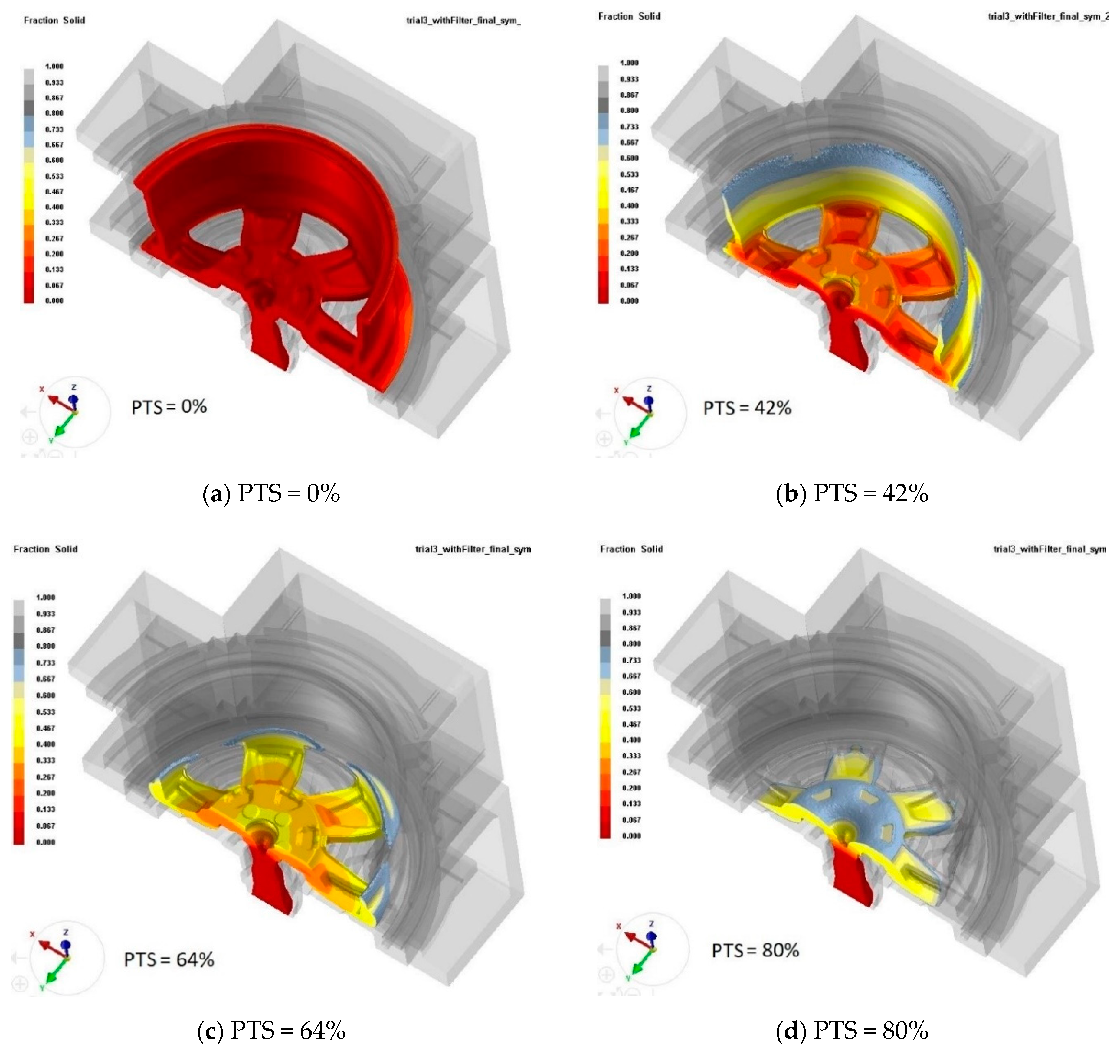
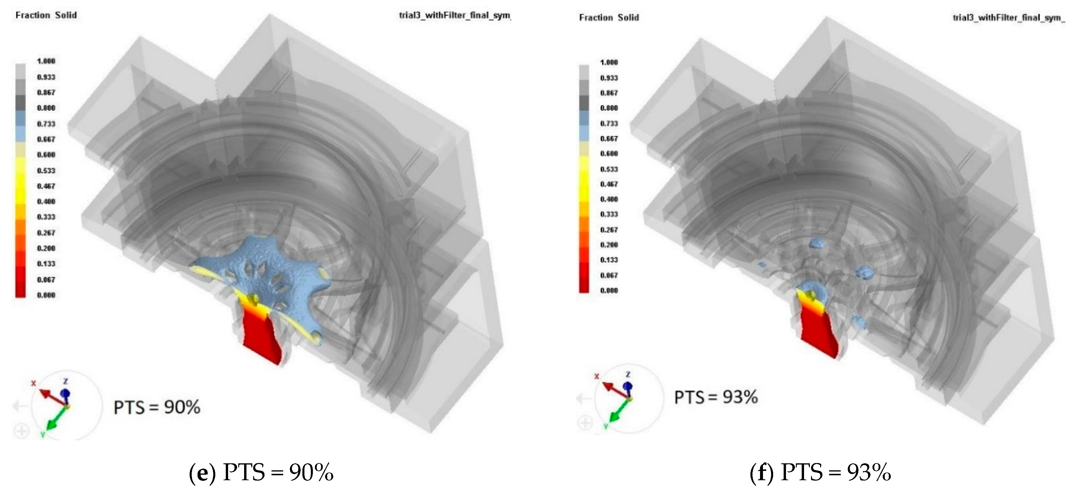
3.3. Solidification Direction

The solidification path predicted by the model has been used to assess the locations that would be prone to form porosities. The solidification front should ideally follow a path that continuously provides access to liquid to offset the density increase associated with the liquid-to-solid transformation. The failure to achieve this condition may lead to the formation of regions containing partially solidified material that is “shut-off” from a supply of liquid and encapsulated in solid. Depending on the structural integrity of the surrounding solid, the cleanliness of the liquid metal (e.g., oxide films) and the hydrogen content in solution in the liquid metal, this could result in the formation of distributed porosity (e.g., shrinkage- or hydrogen-based) or surface depressions/deformation.
Focusing first on the production process condition, Figure 16 presents a series of images (a–f) of the wheel within the die at increasing times within the cast cycle. In each image, the portion of the wheel with a solid fraction, fs, greater than 0.7 is removed or “cut-off” in the image, thereby allowing the progress of the solidification front within the die to be observed. As can be seen in the series of images, in general the solidification front follows a path from the upper die (in-board rim flange) to the sprue. Small volumes of liquid encapsulated (~18 mm in equivalent radius) can be seen at the spoke/hub junction in image (f), at PTS (percentage of total solidification) = 93%. A close-up view of the bottom die structure in the vicinity of the area of liquid encapsulation is shown in Figure 17. As can be seen, the structure of the die is complex, resulting in a large surface area for heat transfer per volume of material undergoing solidification, likely leading to the formation of the region of encapsulation. As presented in Section 4.1.5 in reference [17], no noticeable shrinkage-based porosity was observed in the area in question from the line-of-sight X-ray images taken of example wheels cast under the production process condition in a cyclic steady state. This indicates that either the model falsely predicted the area of liquid encapsulation, or alternatively the size of the porosity was below the threshold for detection in the X-ray imaging system used.
Turning to the non-production process condition, only the stages with the formation of liquid encapsulation are presented in Figure 18 for brevity. It can be seen that liquid encapsulation formed in two regions: the rim/spoke junction at PTS = 85%, and the spoke/hub junction at PTS = 94%. The former is ~27 mm in equivalent radius, whereas the latter has a similar location and size (~16 mm in equivalent radius) to that predicted in the production process condition wheel. Compared to the X-ray radiography results [17], Figure 19, with the larger area of liquid encapsulation predicted by the model, indicates consistency. This lends some support to the conclusion that the other smaller areas of liquid encapsulation yielded porosities below the detection limit.

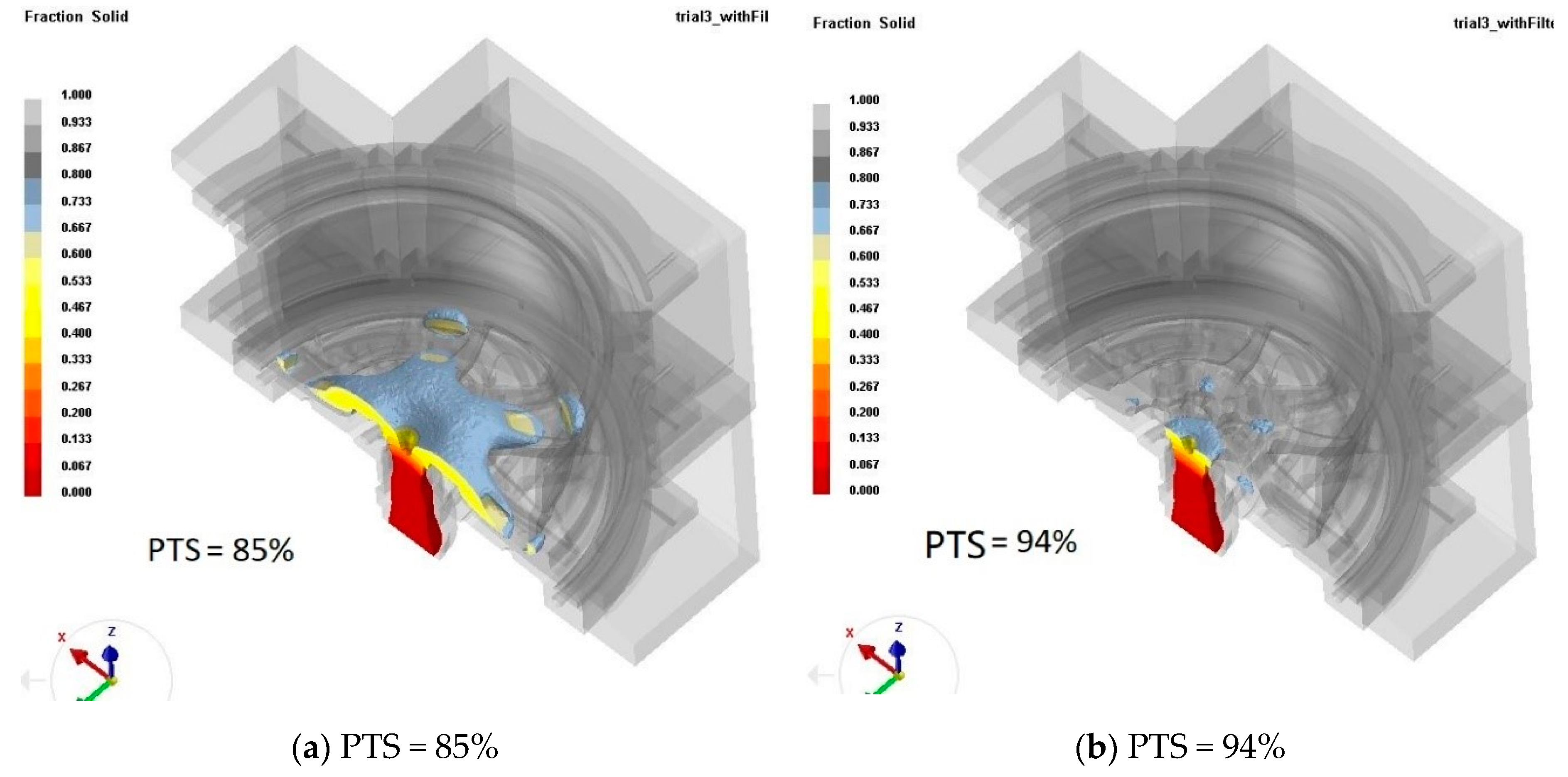
3.4. Further Validation on Die-B

In order to further evaluate the robustness of this modeling methodology, a second die structure (Die-B) was simulated. Temperature data have also been acquired from the die in a production setting and compared to the model predictions. Figure 20 displays the geometry of the second wheel. This is a conventional LPDC 17 × 7 in, 10-spoke wheel, and the die for producing this wheel was cooled by water only. The standard production parameters were used for the plant trial. Note: in comparison, the wheel produced by Die-A is a conventional 17 × 7.5 in, 6-spoke wheel, and the die was cooled by both water and air.

Model Validation

Figure 21 presents the comparison between the measured data and model predictions for the in-die temperatures (the error, T e r r o r , in Figure 22), and the comparison of in-wheel temperatures in Figure 23. The locations of the TCs are shown in Figure 24. As can be seen from the comparison, the model is able to reproduce the behavior observed at the various locations within the die and wheel selected for the comparison accurately. By comparing the temperature error of this case (Figure 22) to the other two process conditions (Figure 9 and Figure 11), it can be seen that the accuracy does not degrade (the maximum   T e r r o r is only ~23 °C at BD55). It is worthwhile to mention again that the model parameters were not re-tuned for the analysis of Die-B. This result provides evidence to support the robustness of the modeling methodology, insofar as the model is able to capture the key phenomena governing the transport of heat independently of die geometry and the cooling conditions within the range encompassed by the two wheel/die combinations examined. The result also bodes well for the model being able to accurately predict a broader range of die/wheel geometries.

4. Summary

An advanced modeling methodology has been developed using the commercial software package ProCAST for the industrial LPDC-based production of aluminum alloy A356 automotive wheels. The methodology incorporates the relevant material properties, the boundary conditions to characterize interfacial heat transfer associated with the various interfaces in the process (including die/wheel, die/die, die/cooling water and die/cooling air), and the latent heat associated with solidification. The model has been comprehensively validated using in-die and in-wheel temperature data collected from a commercial production casting machine operating at steady state. Aspects of the methodology developed to describe the die/cooling water interface boundary condition benefited significantly from in-channel water temperature data, which indicated the presence of periods of boiling water heat transfer, both when water is first introduced to the channel and after the application of purging air.
The validation was carried out over a range of process conditions, including (1) production process conditions for Die-A, (2) non-production process conditions for Die-A, and (3) production process conditions for a second die structure, Die-B. The model was originally developed and some interface conditions were “tuned” based on analysis of the production conditions for Die-A. The model was then applied without re-tuning to a second set of process conditions (non-production), in which the cooling channel timing was significantly altered. Finally, the model was applied to a second die structure, Die-B, also without retuning. In addition to changes in geometry, the process conditions for Die-B were different in two ways: (1) the cooling timing was different, and (2) the die contained only water-cooling elements, unlike Die-A which utilized both air- and water-cooling elements.
The comparisons presented between the in-process-derived TC data and the model predictions indicated that the model is able to reproduce the temperature evolution at the locations examined in the wheel and die accurately for the range of process conditions/die structures examined in the study, without the need for re-tuning. Comparisons to X-ray images taken of wheels produced from Die-A for the non-production process condition indicate that the model is able to predict the location of shrinkage-based porosity associated with pockets of encapsulated liquid of ~2 m equivalent radius. Other areas of encapsulated liquid predicted by the model, for both the production and non-production process conditions, that were smaller in size (~16 to 18 mm in equivalent radius) did not appear to have shrinkage porosity associated with them, according to the X-ray images. It was suggested that this may be due to limits in the resolution of the line-of-sight X-ray images used to detect smaller clusters of shrinkage porosity. Additional work is required to investigate this further.

Author Contributions

Methodology, J.O., D.M. and S.C.; investigation, J.O., C.W., D.M. and S.C.; model development, J.O., C.W. and L.Z.; resources, Z.Z., L.A. and C.L.; writing—original draft preparation, J.O.; writing—review and editing, C.W., S.C., D.M., L.Z., L.A., C.L. and Z.Z.; supervision, S.C., D.M., L.A., C.L. and Z.Z.; All authors have read and agreed to the published version of the manuscript.

Funding

This research was funded by CITIC Dicastal Co., Ltd. (Qinhuangdao, China).

Acknowledgments

The authors would like to thank CITIC Dicastal Co., Ltd. for funding support and access to facilities and personnel.

Conflicts of Interest

The authors declare no conflict of interest. The sponsor had no role in the design, execution, interpretation, or writing of the study. The sponsor has reviewed the manuscript to ensure confidential information is not being released.

References

  1. Bonollo, F.; Urban, J.; Bonatto, B.; Botter, M. Gravity and low pressure die casting of aluminium alloys: A technical and economical benchmark. la Metall. Ital. 2005, 97, 23–32. [Google Scholar]
  2. Isenstadt, A.; German, J.; Bubna, P.; Wiseman, M.; Venkatakrishnan, U.; Abbasov, L.; Guillen, P.; Moroz, N.; Richman, D.; Kolwich, G. Lightweighting technology development and trends in US passenger vehicles. Int. Counc. Clean Transp. Work. Pap. 2016, 25, 1–24. [Google Scholar]
  3. Sun, J.; Le, Q.; Fu, L.; Bai, J.; Tretter, J.; Herbold, K.; Huo, H. Gas entrainment behavior of aluminum alloy engine crankcases during the low-pressure-die-casting process. J. Mater. Process. Technol. 2019, 266, 274–282. [Google Scholar] [CrossRef]
  4. Sui, D.; Cui, Z.; Wang, R.; Hao, S.; Han, Q. Effect of cooling process on porosity in the aluminum alloy automotive wheel during low-pressure die casting. Int. J. Met. 2016, 10, 32–42. [Google Scholar] [CrossRef]
  5. Thomas, B.G. Review on Modeling and Simulation of Continuous Casting. Steel Res. Int. 2018, 89, 1700312. [Google Scholar] [CrossRef]
  6. Hetu, J.F.; Gao, D.M.; Kabanemi, K.K.; Bergeron, S.; Nguyen, K.T.; Loong, C.A. Numerical modeling of casting processes. Adv. Perform. Mater. 1998, 5, 65–82. [Google Scholar] [CrossRef]
  7. Merlin, M.; Timelli, G.; Bonollo, F.; Garagnani, G.L. Impact behaviour of A356 alloy for low-pressure die casting automotive wheels. J. Mater. Process. Technol. 2009, 209, 1060–1073. [Google Scholar] [CrossRef]
  8. Duan, J.; Maijer, D.; Cockcroft, S.; Reilly, C. Development of a 3D Filling Model of Low-Pressure Die-Cast Aluminum Alloy Wheels. Metall. Mater. Trans. A 2013, 44, 5304–5315. [Google Scholar] [CrossRef]
  9. Fan, P.; Cockcroft, S.; Maijer, D.; Yao, L.; Reilly, C.; Phillion, A. Examination and Simulation of Silicon Macrosegregation in A356 Wheel Casting. Metals 2018, 8, 503. [Google Scholar] [CrossRef] [Green Version]
  10. Fan, P.; Cockcroft, S.L.; Maijer, D.M.; Yao, L.; Reilly, C.; Phillion, A.B. Porosity Prediction in A356 Wheel Casting. Metall. Mater. Trans. B Process Metall. Mater. Process. Sci. 2019, 50, 2421–2435. [Google Scholar] [CrossRef]
  11. Moayedinia, S. Quantification of Cooling Channel Heat Transfer in Low Pressure Die Casting; University of British Columbia: Vancouver, BC, Canada, 2014. [Google Scholar]
  12. Sengupta, J.; Thomas, B.G.; Wells, M.A. Understanding the role water-cooling plays during continuous casting of steel and aluminum alloys. In Proceedings of the Materials Science &Technology 2004, New Orleans, LA, USA, 26–29 September 2004; Volume 2, pp. 179–193. [Google Scholar]
  13. Fackeldey, M.; Ludwig, A.; Sahm, P.R. Coupled modelling of the solidification process predicting temperatures, stresses and microstructures. Comput. Mater. Sci. 1996, 7, 194–199. [Google Scholar] [CrossRef]
  14. Griffiths, W.D.; Kawai, K. The effect of increased pressure on interfacial heat transfer in the aluminium gravity die casting process. J. Mater. Sci. 2010, 45, 2330–2339. [Google Scholar] [CrossRef]
  15. Zhang, B.; Maijer, D.M.; Cockcroft, S.L. Development of a 3-D thermal model of the low-pressure die-cast (LPDC) process of A356 aluminum alloy wheels. Mater. Sci. Eng. A 2007, 464, 295–305. [Google Scholar] [CrossRef]
  16. Zhang, L.; Wang, R. An intelligent system for low-pressure die-cast process parameters optimization. Int. J. Adv. Manuf. Technol. 2013, 65, 517–524. [Google Scholar] [CrossRef]
  17. Ou, J.; Wei, C.; Cockcroft, S.; Maijer, D.; Zhu, L.; A, L.; Li, C.; Zhu, Z. Advanced Process Simulation of Low Pressure Die Cast A356 Aluminum Automotive Wheels—Part I, Process Characterization. Metals 2020, 10, 563. [Google Scholar] [CrossRef]
  18. Mills, K.C. Recommended Values of Thermophysical Properties for Selected Commercial Alloys; Woodhead Publishing: Cambridge, UK, 2002. [Google Scholar]
  19. Thompson, S.; Cockcroft, S.L.; Wells, M.A. Advanced light metals casting development: Solidification of aluminium alloy A356. Mater. Sci. Technol. 2004, 20, 194–200. [Google Scholar] [CrossRef]
  20. Lucefin Group 34CrMo4 Properties. Available online: http://www.lucefin.com/wp-content/files_mf/0334crmo4.pdf (accessed on 21 October 2020).
Figure 1. Mesh of the wheel produced with Die-A.
Metals 10 01418 g001
Figure 2. Temperature-dependent thermophysical properties of A356.
Metals 10 01418 g002
Figure 3. Temperature-dependent thermophysical properties of H13 tool steel.
Metals 10 01418 g003
Figure 4. Temperature-dependent thermophysical properties of 34CrMo4 (German designation).
Metals 10 01418 g004
Figure 5. Schematic profile of the HTCs applied at the casting/die interface.
Metals 10 01418 g005
Figure 6. An example of the calculated HTC applied at the cooling channel in side die.
Metals 10 01418 g006
Figure 7. Locations of the cooling channels and TCs (a), and the photo showing the TC installation at the top die (b).
Metals 10 01418 g007
Figure 8. Temperature comparison between the model and measured data for the production process condition in Die-A.
Metals 10 01418 g008aMetals 10 01418 g008b
Figure 9. Error between the model and measured data.
Metals 10 01418 g009
Figure 10. Temperature comparison between the model and measured data for the non-production process condition in Die-A.
Metals 10 01418 g010
Figure 11. Error between the model and measured data.
Metals 10 01418 g011
Figure 12. Time average temperature difference between production and non-production conditions for the in-process derived data and model predictions in Die-A.
Metals 10 01418 g012
Figure 13. Temperature measured within the cooling channel T3 by TC TD21 in Die-A.
Metals 10 01418 g013
Figure 14. In-wheel temperature comparison for (a) production and (b) non-production process conditions in Die-A.
Metals 10 01418 g014
Figure 15. Cast-in TC locations in wheels produced with Die-A.
Metals 10 01418 g015
Figure 16. Solidification path for the production process condition.
Metals 10 01418 g016aMetals 10 01418 g016b
Figure 17. Geometric features of the bottom die for producing the bolt holes in the wheel in Die-A.
Metals 10 01418 g017
Figure 18. Solidification path for the non-production process condition.
Metals 10 01418 g018
Figure 19. Large size shrinkage-based porosity found at the rim/spoke conjunction.
Metals 10 01418 g019
Figure 20. Wheel geometry and mesh (469,100 2D elements and 2,896,039 3D elements) used for additional model validation (Die-B).
Metals 10 01418 g020
Figure 21. In-die temperature comparison between the model and measured data for the second die/wheel geometry.
Metals 10 01418 g021
Figure 22. Error between the model and measured data.
Metals 10 01418 g022
Figure 23. In-wheel temperature comparison between the model and measured data for the second die/wheel geometry.
Metals 10 01418 g023
Figure 24. TC locations.
Metals 10 01418 g024
Table 1. Components and their materials.
ComponentMaterial
WheelA356
Die structure (except side dies)H13 tool steel
Side dies35CrMo steel
Table 2. Chemical composition of 35CrMo, 34CrMo4 and H13.
MaterialCSiMnCrMoVFe
35CrMo (Chinese designation)0.32–0.40.17–0.370.4–0.70.8–1.10.15–0.25-Bal.
34CrMo4 (German designation)0.3–0.37max 0.40.6–0.90.9–1.20.15–0.3-Bal.
H13 tool steel0.32–0.450.8–1.250.2–0.64.75–5.51.1–1.750.8–1.2Bal.
Table 3. HTCs specified for the casting/die interfaces.
InterfaceHTC
W/(m2 K)
Liquid/SolidSolid/Solid
Casting/Top Die1400700
Casting/Side Die1400280
Casting/Bottom Die1750210
Table 4. HTCs at the die/die interfaces.
InterfaceHTC
W/(m2 K)
Top die/Side die800
Top die/Bottom die1000
Bottom die/Side die500
Side die/Side die500
Table 5. Parameters for the environmental heat transfer.
RegionProcess ConditionHTCEmissivity T e n v
W/(m2 K)°C
Top dieProduction200.8150–200 **
Non-Production *70
Side diesBoth conditions200.825–140 **
Bottom dieProduction200.8150
Non-Production *70
* The duration of air cooling under the non-production process condition is significantly longer than the production process condition which decreases the environment temperature, T e n v , and thus the cooling efficiency increases. To standardize the model parameters, instead of changing T e n v , proportionally greater HTCs are used for the non-production process condition. ** Depending on the reference die components, different T e n v are applied at different locations of the surface based on measured data from the production process condition.
Publisher’s Note: MDPI stays neutral with regard to jurisdictional claims in published maps and institutional affiliations.

