
Intelligent Recognition Model of Hot Rolling Strip Edge Defects Based on Deep Learning
by
 ,
,
Dongcheng Wang
1,2,*, 
Yanghuan Xu
1,
Bowei Duan
1,
Yongmei Wang
1,
Mingming Song
1,
Huaxin Yu
1 and
Hongmin Liu
1,2 1
National Engineering Research Center for Equipment and Technology of Cold Rolling Strip, Yanshan University, Qinhuangdao 066004, China
2
State Key Laboratory of Metastable Materials Science and Technology, Yanshan University, Qinhuangdao 066004, China
*
Author to whom correspondence should be addressed.
Metals 2021, 11(2), 223; https://0-doi-org.brum.beds.ac.uk/10.3390/met11020223
Submission received: 16 December 2020
/
Revised: 19 January 2021
/
Accepted: 22 January 2021
/
Published: 27 January 2021
(This article belongs to the Special Issue Recent Advances and Applications of Machine Learning in Metal Forming Processes)
Abstract
:The edge of a hot rolling strip corresponds to the area where surface defects often occur. The morphologies of several common edge defects are similar to one another, thereby leading to easy error detection. To improve the detection accuracy of edge defects, the authors of this paper first classified the common edge defects and then made a dataset of edge defect images on this basis. Subsequently, edge defect recognition models were established on the basis of LeNet-5, AlexNet, and VggNet-16 by using a convolutional neural network as the core. Through multiple groups of training and recognition experiments, the model’s accuracy and recognition time of a single defect image were analyzed and compared with recognition models with different learning rates and sample batches. The experimental results showed that the recognition model based on the AlexNet had a maximum accuracy of 93.5%, and the average recognition time of a single defect image was 0.0035 s, which could meet the industry requirement. The research results in this paper provide a new method and thought for the fine detection of edge defects in hot rolling strips and have practical significance for improving the surface quality of hot rolling strips.
1. Introduction
Surface quality is an important indicator of hot rolling strip products. Surface defects not only have an influence on product appearance and rolling yield, but also have a harmful effect on the production of downstream processes [1,2]. Surface defects can be detected quickly and accurately through a surface quality detection system, which has practical significance for improving the surface quality of a strip. A new direction for strip surface quality detection has been provided with the rapid development of artificial intelligence, machine vision theory, and technology [3,4,5,6]. Many scholars have conducted related research.
Xu et al. [7] used eight 1024-pixel linear CCD (Charge Coupled Device) cameras as an image acquisition device and proposed the procedure of defect detection, and a recognition algorithm based on the surface features of a hot rolling strip, which was applied to a 1700 mm hot rolling strip production line. Later, a new method based on Tetrolet transform and kernel locality preserving projection for dimension reduction was proposed to detect the surface defects of hot rolling strips [8], and the recognition accuracy on the defect sample database was 97.3846%. He et al. [9] developed a long-distance and super-bright LED light and solved the problem of inhomogeneous illumination from a long distance at a high temperature. It simultaneously met the illumination request of line scan camera and plane scan camera imaging, and the real-time recognition of the strip surface defects was carried out using the decision tree classification model. Gan et al. [10] used a decision tree and expert experience classification model to recognize silicon steel surface defects. Zhao [11] used the VggNet16 model to recognize silicon steel surface defects, and the accuracies of the model on training and test sets were 97.5% and 92.27%, respectively. Han et al. [12] proposed a surface defect recognition method based on a BP (Back Propagation) neural network, and its accuracy reached more than 84%. Chu [13] used a least square twin support vector machine to recognize strip surface defects with an accuracy of 95.4% while greatly improving the recognition efficiency. Xing [14] improved the AlexNet model constructure, which was used to classify the surface defects of hot rolling strips by adjusting the size and number of convolution kernels with a recognition accuracy of 93.4%. Subsequently, a defect classification and index system based on MATLAB was developed.
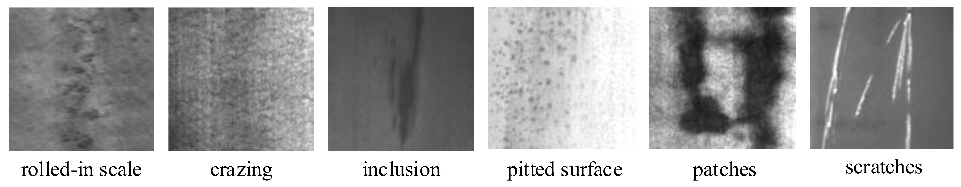
Song et al. [15] established an NEU (Northeastern University) surface defect database, including the six kinds of typical surface defects of hot rolling strips: rolled-in scale (RS), patches (Pa), crazing (Cr), pitted surface (PS), inclusion (In), and scratches (Sc). Subsequently, a robust feature descriptor against noise named the adjacent evaluation completed local binary patterns (AECLBP) was proposed for defect recognition, and its recognition accuracy reached 97.89%. The NEU surface defect database was a significant contribution to the research of strip defect recognition. For instance, Hu [16] compared the recognition performance between AdaBoost and AdaBoost.BK on the NEU surface defect database, and their results showed that AdaBoost.BK had the highest classification accuracy when the backward step was F = 2. Though a long training time was needed, the recognition time of a single defect image was only 0.002132 s. Xie [17] used a deep residual network and transfer learning method, and its recognition accuracy on the NEU surface defect database reached 98.54%, which was better than that of VggNet16. Gao et al. [18,19] adopted a deep residual network and semi-supervised learning method to research the NEU surface defect database. The recognition accuracy of the deep residual network reached 99.889%, and the recognition accuracy of semi-supervised learning reached 86.72%. However, the data label can be omitted in the semi-supervised learning method, which improves the efficiency. This method is more suitable for the defect recognition mission that has a limitation on labeling. Saiz et al. [20] combined traditional machine learning techniques with convolutional neural networks and proposed an automatic classification method of strip surface defects based on a deep learning method. The best classifier parameters were obtained through plenty of experiments, and the robustness of the classifier was verified. The classification time of a single image was only 0.019 s on the NEU surface defect database, thereby achieving a classification accuracy of 99.95%. Lee et al. [21] proposed a relative approach for diagnosing steel defects using a deep structured neural network with class activation maps, and it achieved detection performance values of 99.44% and 0.99 in terms of accuracy and the F-1 score metric, respectively. He et al. [22,23] proposed a generative adversarial network and fused multiple hierarchical feature network defect classification method, respectively, and the recognition accuracy on the NEU surface defect database reached values of 99.56% and 99.67%. Dong et al. [24] proposed a pyramid feature fusion and global context attention network for the pixel-wise detection of surface defect named PGA-Net. The average pixel accuracy of the proposed method on the four defect datasets was 92.15% for NEU-Seg, 74.78% for DAGM 2007, 71.31% for MT_defect, and 79.54% for Road_defect, all of which were better than existing methods. Guan et al. [25] evaluated the image quality of the potential feature information of a strip defect through visualization and proposed a strip surface defect classification algorithm. Compared with VggNet19 and ResNet, the proposed method had a better performance in terms of prediction accuracy and speed on the NEU surface defect database. Fu et al. [26] proposed a lightweight convolutional neural network (CNN) defect recognition model that emphasized the training of low-level features and incorporated multiple receptive fields to achieve fast and accurate classification on the NEU surface defect database. The model could realize real-time detection, and its running speed could reach 100 fps in computer equipped with single NVIDIA TITAN X and 12G RAM (Random Access Memory).
In summary, the existing detection equipment, theories, and techniques of hot rolling strip surface defects have basically achieved a satisfactory performance for typical defects with obvious features (e.g., crazing, inclusion, patches, scratches, rolled-in scale, and pitted surface). However, the strip edges (approximately 50 mm on both sides) are frequent areas of surface defects in production practice. Common defects include upwarps, black lines, cracks, slag inclusions, and gas holes. The generation mechanisms and corresponding solutions of these defects vary, but the macroscopic features are relatively similar, and the online surface quality detection system often recognizes them as the same type of defect. To eliminate concrete defects, the production line generally needs to further subdivide defects through manual detection, which seriously reduces production efficiency and increases labor intensity. To this end, the authors of this article subdivided the edge defects of a hot rolling strip into five types and the intelligent recognition model of edge defects was investigated.
2. Convolutional Neural Network Recognition Model for Edge Defects
2.1. Characteristics of Edge Defects
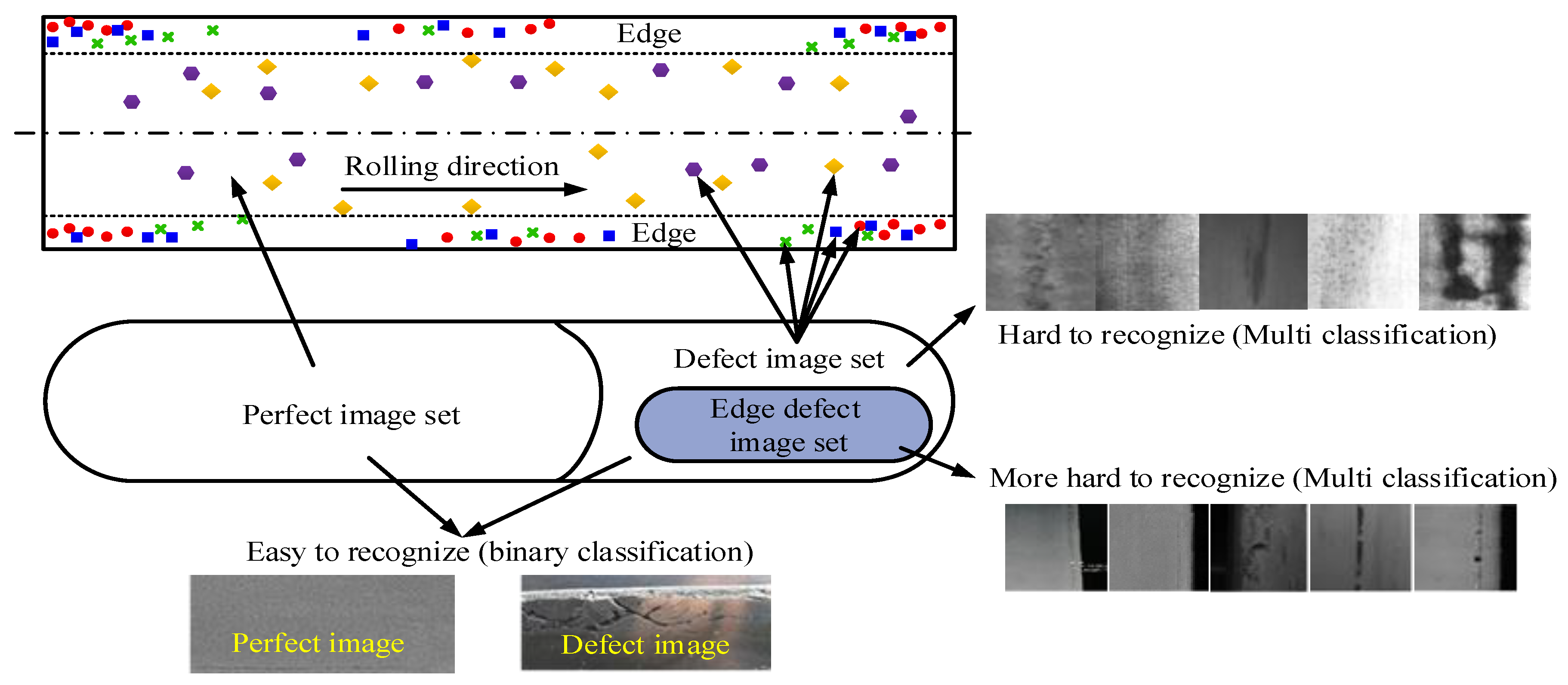
As shown in Figure 1, during the actual production process of hot rolling strips, surface defects often appear. There are many types of defects, and these defects often occur in the head, tail, and both sides of the strip. Frequently, the feature difference between a perfect image and a defect image is obvious. Traditional machine vision theory can be used to solve this binary classification problem, and it is not difficult for a surface quality detection system to complete this task. However, there are some problems when classifying defect images. Because the feature difference among the various defects is not obvious, traditional machine vision theory cannot perform well to complete this multi classification problem. For this reason, many scholars have tried to solve this problem by using deep learning neural networks [15,22,23,24]. The edge defects are more special in a defect image set. The various edge defects generally have similar linear features, and a surface quality detection system often classifies these different types of defects into one classification, which is not conducive to the further analysis of the defect generation mechanism and the proposition of corresponding solutions. The authors of this paper took the edge defect set as the research object and studied the recognition model of edge defect image based on a convolutional neural network. The purpose was to improve the recognition accuracy of edge defects.
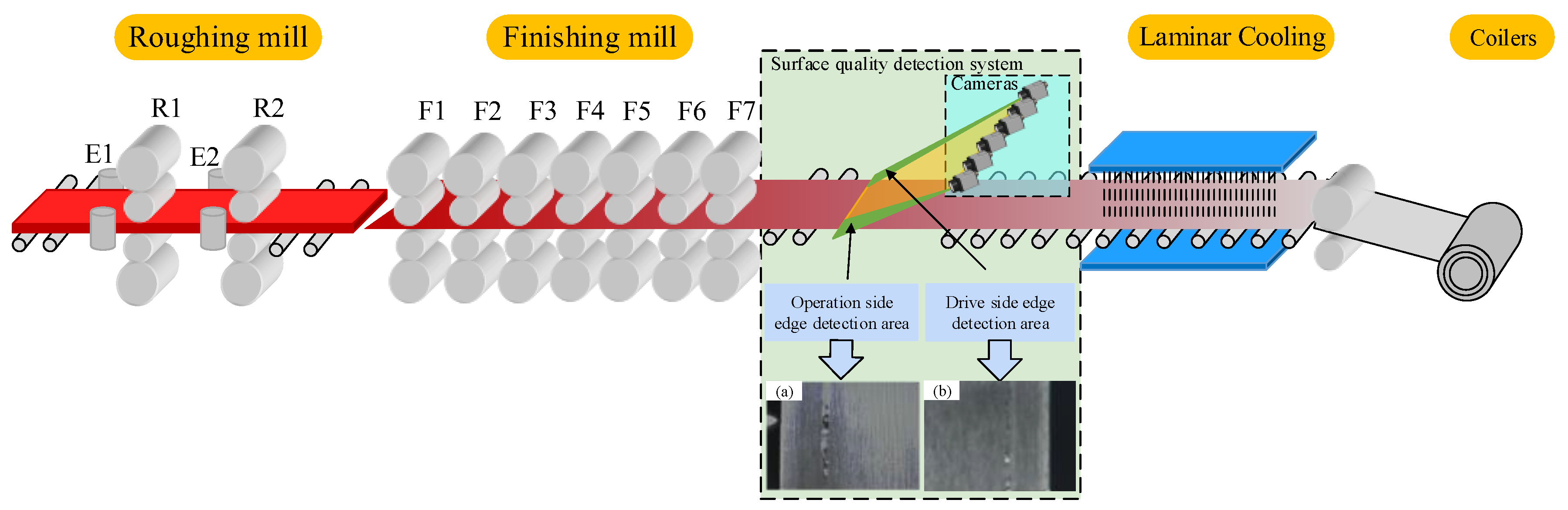
The edge defects of a hot rolling strip occur on the operation and drive sides of the strip. The defects are detected by cameras on both edge sides of the surface quality detection system (SQDS). The detection position is located between the exit of the finishing mill’s seventh stand and laminar cooling areas (Figure 2). These edge defects are evolved by heating, rough rolling, finishing rolling, and other processes. The evolution process is shown in Figure 3. In practical production, each defect must be accurately detected, and effective control method must be carried out.
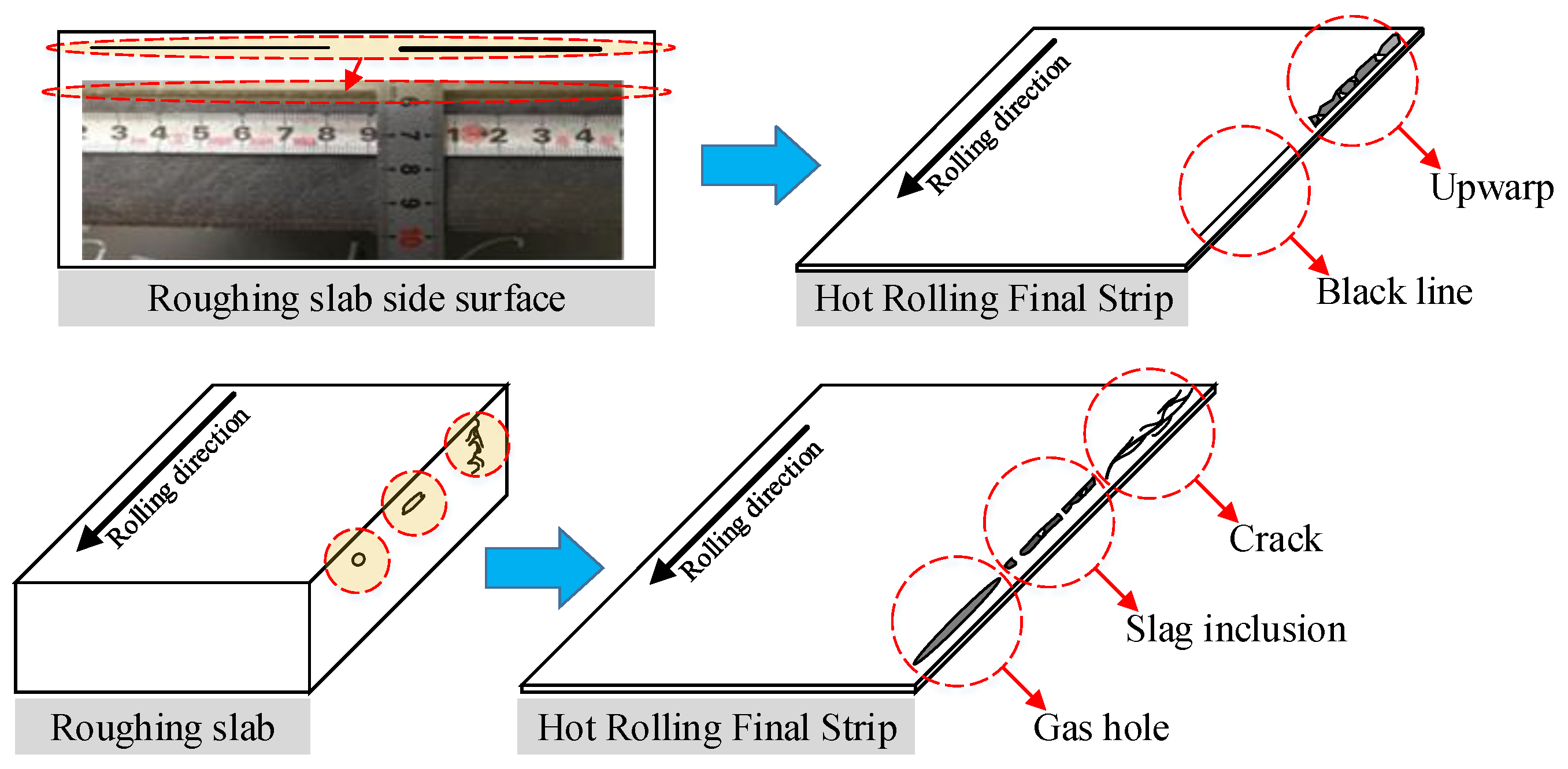
Take the upwarp as an example. This defect often appears in IF (Interstitial-Free) steel. The generation mechanism of the defect is the temperatures in the edge and corner of the intermediate slab drop too fast during the hot rolling process, so the γ→α phase transformation is likely to occur in advance, thus resulting in an uneven distribution of flow stress and transverse flow in the thickness direction of the intermediate slab. The side of intermediate slab forms a large fold. As the rolling process continues, this large fold flips to the surface of the strip and forms edge upwarp [27,28]. In actual production, once the edge upwarp occurs, the temperature of the heating furnace should be appropriately increased, and an edge heater should be turned on at the same time so that the large folds in edge and corner of intermediate slab of subsequent products can be eliminated to avoid the occurrence of edge upwarp.
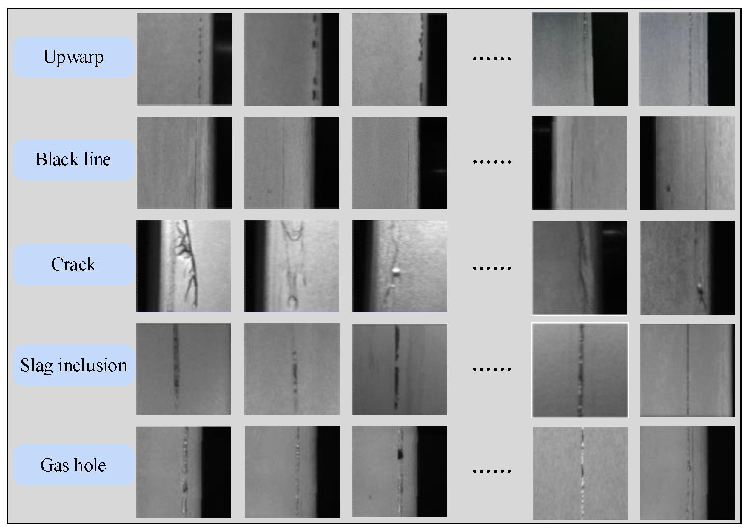
In this paper, after long-term tracking, sampling analysis, and technique exchanges for a 2250 mm hot rolling production line, the edge defects were divided into five types, namely upwarp, black line, crack, slag inclusion, and gas hole. The length, width, and specific features of these five types of defects are shown in Table 1. Table 1 shows that, except for the crack, the features of the four other types of defects presented a certain linear feature, but the line’s width, length, color, and specific texture features were not completely consistent. Among them, the upwarp and black line were found to have the same generation mechanism, and their features reflected a certain similarity. Thus, they both belong to the edge seam defects [27,28]. However, because of the different severities of the two types of defects, they were divided into two types during the recognition process. Meanwhile, the images of slag inclusion and gas hole easily caused confusion, and detection errors of these two types of defects often occurred. Compared with other typical surface defects of hot rolling strips (e.g., crazing, inclusion, patches, scratches, rolled-in scale, and pitted surface) (Figure 4 [15]), the detection of edge defects is relatively difficult.
2.2. Convolutional Neural Network Model of Edge Defects
Traditional machine vision or deep learning intelligent methods can be used to achieve the automatic and high-precision detection of the edge defects of hot rolling strips. They are prone to confusion because of the similarity of edge defect features. If traditional machine vision methods are used to extract, segment, or classify defects’ features, obtaining a high recognition accuracy or a strong generalization and perception ability is difficult for the model. As artificial intelligence and deep learning theories are developing, the technology of image detection with a strong similarity is resulting in better performance, such as for face recognition and medical diagnosis [29,30]. However, a CNN, which is a mature deep learning algorithm, has shown excellent performance in many application fields [31,32,33]. The CNN introduces the convolution linear operation, thereby making it more suitable for processing data similar to a network structure, such as time series and image data. Therefore, according to the defect images taken by an surface quality detection system, this article investigated the intelligent recognition of the edge defects of hot rolling strips based on a CNN.
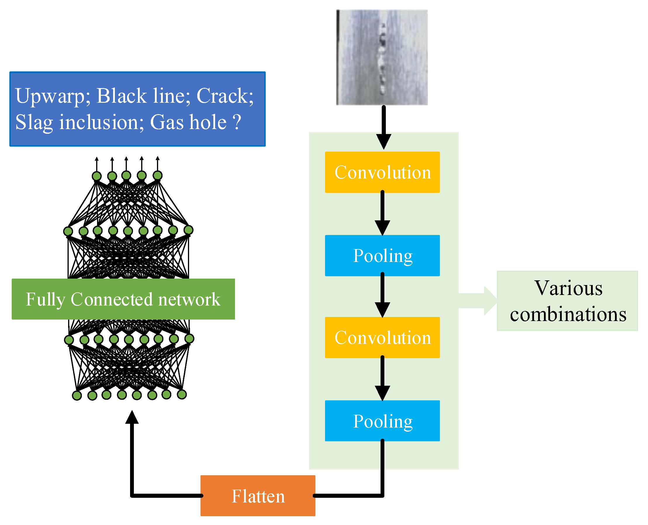
The structure of the CNN recognition model for hot rolling strip edge defect is shown in Figure 5, which includes a data input layer, multiple sets of convolutional and pooling layers, a fully connected feedforward neural network layer, and an output recognition layer. After the original edge defect image data were subjected to multiple convolutional layers, pooling layers, and a nonlinear activation function mapping operation, the feature information was extracted layer by layer. Finally, the probability of image classification was calculated by the fully connected output layers, and the specific classification of defect images was obtained.
- (1)
- Input layer
The input layer uses the edge defect images taken by the surface quality detection system of a hot rolling production line. According to the image size, the model numerically characterizes the internal information of defect images, which is used for the subsequent process and training network.
- (2)
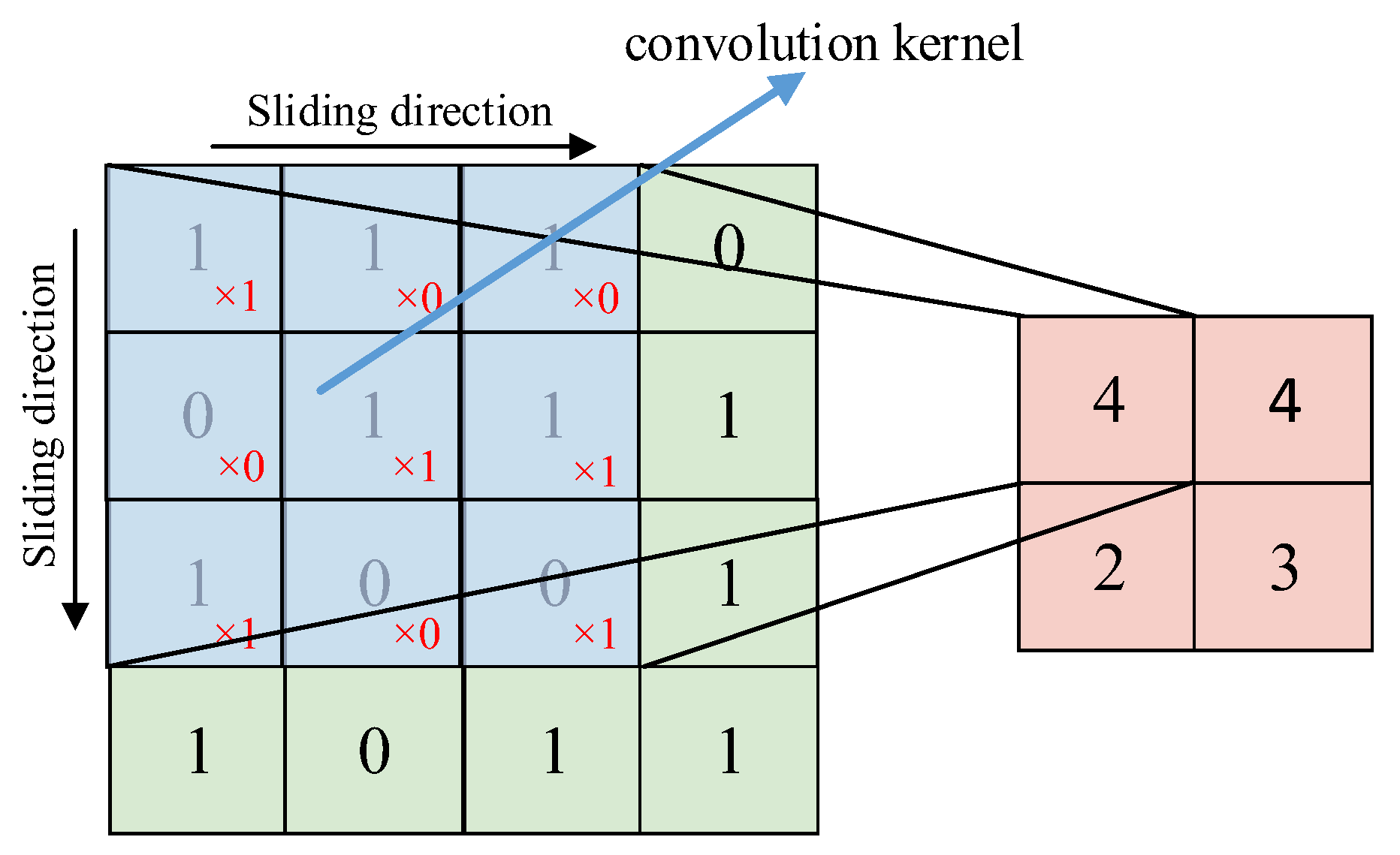
- Convolutional layer
The convolutional layer is the core part of the CNN structure. The image features can be extracted through the convolution operation between a group of convolution kernel and input data. Figure 6 shows that during the whole operation process, the convolution kernel slides from left to right for a specified step and implements the convolution operation with the image data of the input layer. When it reaches far right, it returns to the far-left, slides down for a specified step, and continuously slides from left to right until the whole operation is completed. The size of the feature maps obtained by the convolution operation is related to the parameters, such as the original input image size, convolution kernel size, slide step, and padding size. Assuming that the size of the convolution kernel is , the original input image size is , the slide step is , the padding pixel is , and the output size of the feature maps through the convolution operation is . The calculation formula is presented in Equation (1).
where represents the rounding down operation.
The convolution kernel performs the convolution operation with the previous layer through weight sharing to obtain different feature maps. The more convolution kernels, the stronger the ability to extract the features of the input image. The convolution operation formula is described as Equation (2).
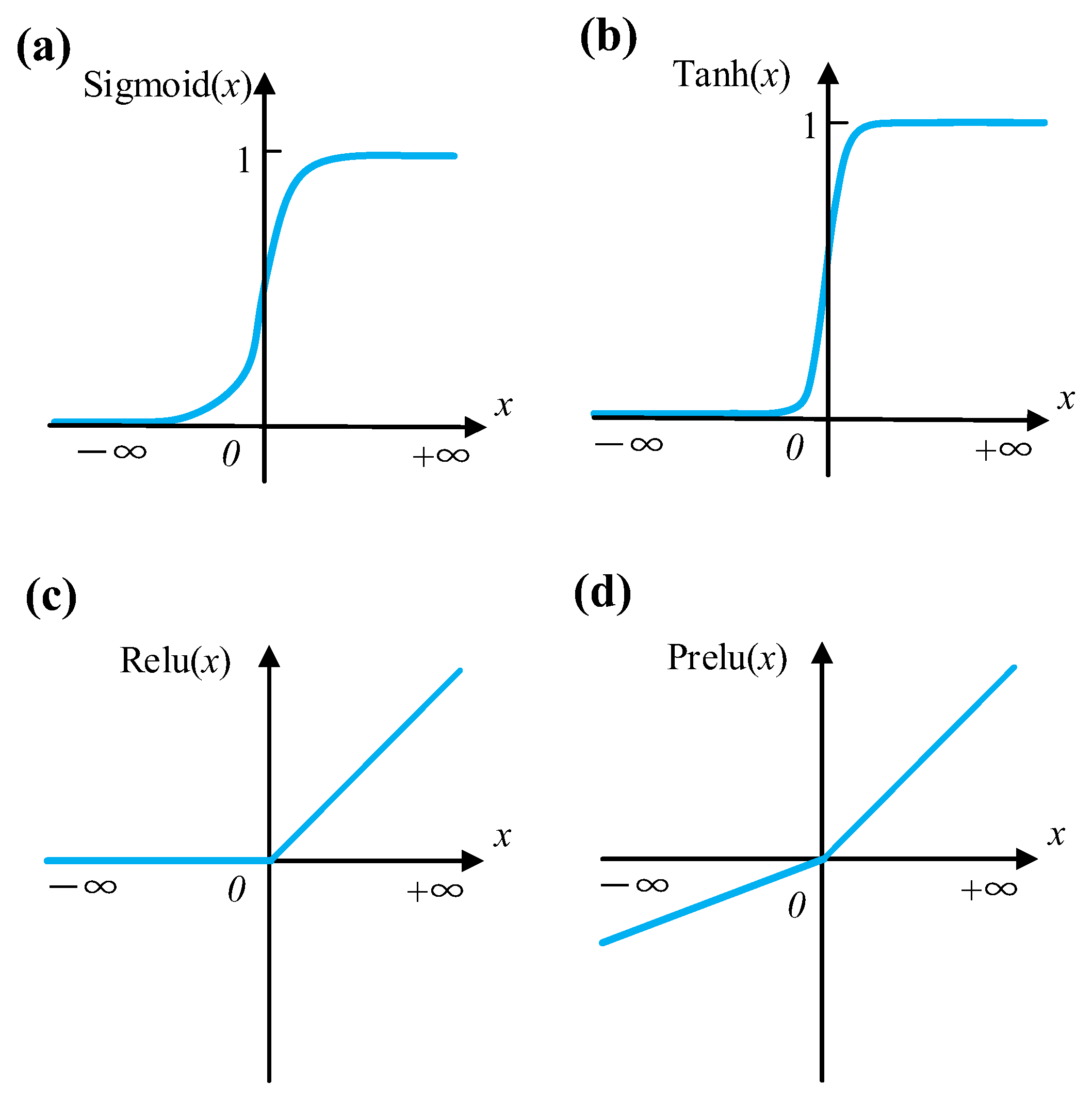
where is the jth output feature map of the lth layer, is the input feature map of the th layer, is the feature map set of the th layer, is the weight from the ith feature map to the jth feature map of the lth layer, is the bias of the jth feature map of the lth layer, and is the activation function. To achieve a nonlinear description of the model after the convolution operation, an activation function is required to implement the nonlinear operation on the linear result, which can enhance the expressive ability of the network model. At present, the commonly used activation functions include: sigmoid, tanh, relu, and prelu. The expression of these activation functions are described in Equations (3)–(6), and their function images are shown in Figure 7.
- (3)
- Pooling layer
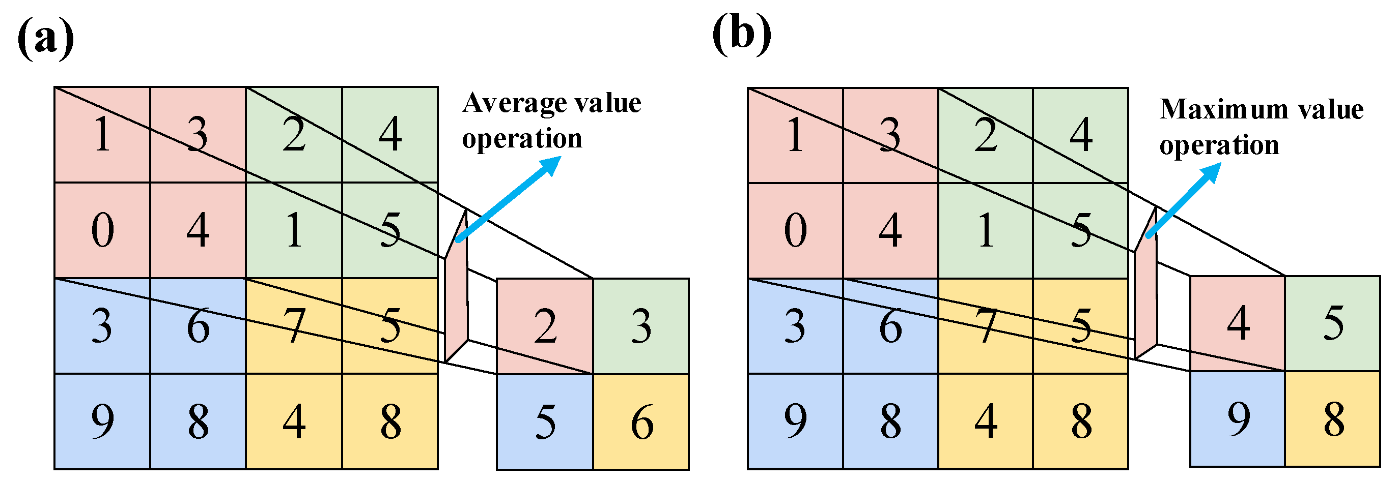
The pooling layer is a down-sampling operation that is usually located after the convolutional layer, and the typical feature information is obtained by down-sampling the original size feature map. Figure 8 shows two commonly used pooling methods, namely max-pooling and average-pooling. The average-pooling takes the average value of the data in the pooling window as the pooling result, and the max-pooling takes the maximum value of the data in pooling window as the pooling result. The max-pooling method is used in most cases. Assuming that the input size of the feature map is , the window size of pooling zone is , the slide step is , and the output size of feature map is . The calculation formula of and is described as Equation (7).
where represents the rounding down operation, and the general value is 2.
- (4)
- Fully connected layer
The fully connected layer integrates all the feature informations extracted from previous convolutional and pooling layers. Each neuron in the fully connected layer connects all neurons in the previous layer, and the calculation formula is described as Equation (8).
where is the output of the fully connected layer, which is a one-dimension vector; is the input of the fully connected layer, which is the feature map values after the convolution and pooling operation; is the weight of the network model; is the bias of the network model; and is the activation function.
- (5)
- Output layer
The last layer of the model is the output recognition layer. The output of multiple neurons is mapped to (0,1) through the Softmax function; its value represents the probability that the input image belongs to this classification. If the input of Softmax is , then the output probability of the defect classification by Softmax function can be described as Equation (9).
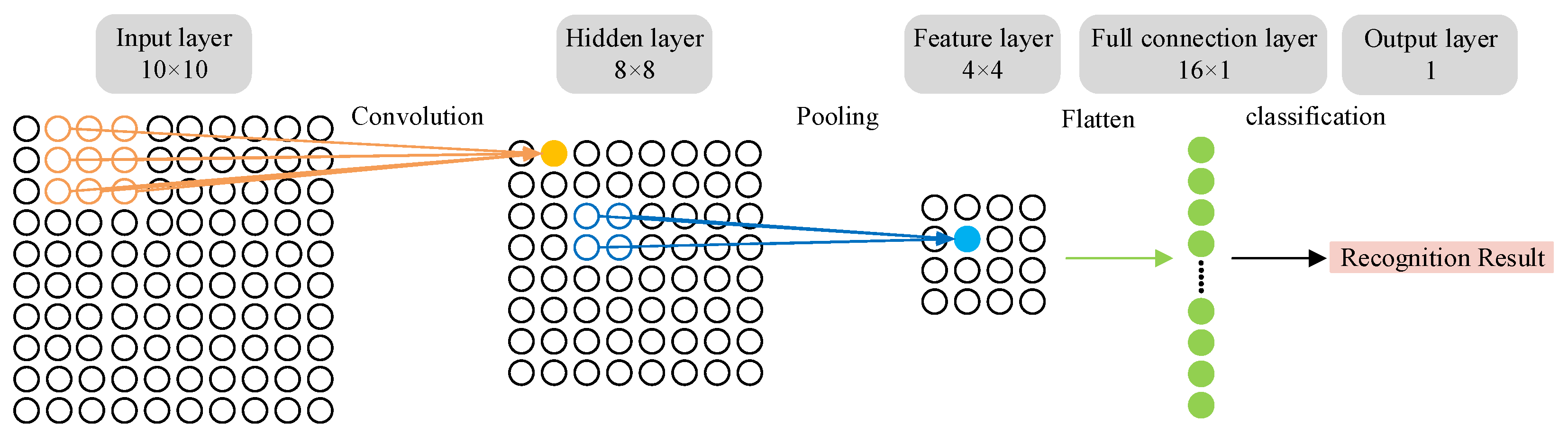
Figure 9 shows the basic process of the CNN. We assumed that the input image data was a 10 × 10 matrix, the size of convolution kernel was 3 × 3, the slide step was 1, and the padding pixel was 0. Through Equation (1), the size of the feature map (hidden layer) obtained from the convolution operation was found to be 8 × 8. The size of the pooling zone was set as 2 × 2, and the slide step was 1. Subsequently, through the further operation of Equation (7), the size of the feature map was found to be 4 × 4. After the flatten operation, the size of the fully connected layer became 16 × 1, and the recognition result was outputted through classification. The CNN had various structures through the combination of different convolutional layers, pooling layers, and different numbers of fully connected layers. Different structures of CNNs have different levels of learning ability for different features. For this, the corresponding experiments had to be implemented for different, specific, and practical problems to ensure a better performance for learning and prediction capability.
3. Experiment and Analysis
3.1. Edge Defect Dataset
Taking the five aforementioned types of edge defects as the research object, the edge defect dataset was collected and produced at the hot rolling production line (Figure 10). The total of 2000 edge defect images were found in the dataset, and 400 images were found in each type of defect. After pre-processing, the size of each image in the dataset was unified to 100 × 100. According to the specified proportion, the dataset was divided into three parts, namely training, validation, and test sets. The image distribution of each part is shown in Table 2. The training and validation sets were used for training the model, whereas the test set was used to verify the learning and generalization abilities of the model, and was not used in model training.
3.2. Experimental Process
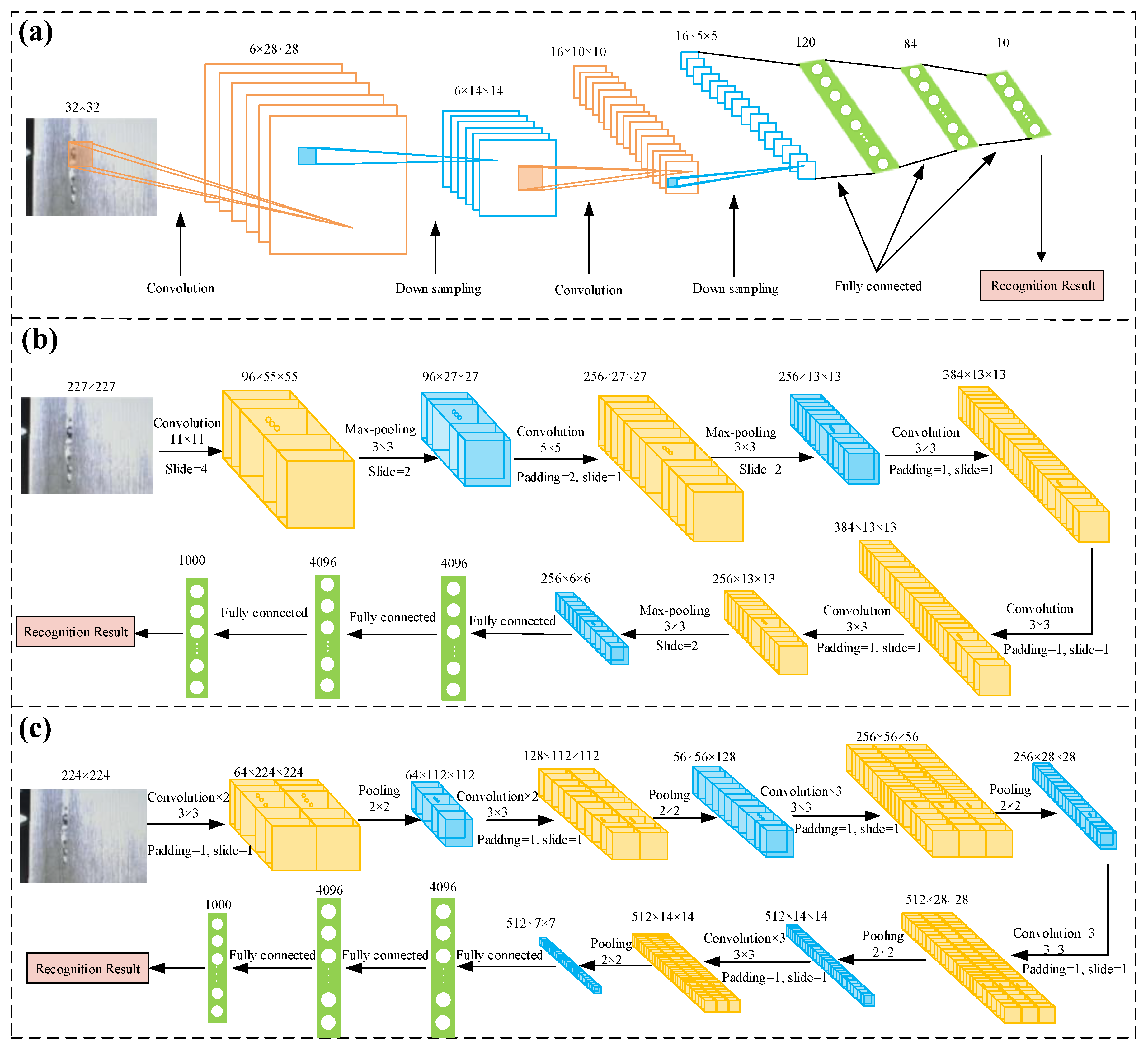
At present, when dealing with different practical problems, there is no uniform principle for how to select and determine the structure of a CNN. Therefore, in this paper, three representative CNN structures, namely LeNet-5, AlexNet, and VggNet-16 [34,35,36], were used to establish the edge defect recognition model for the hot rolling strip. Corresponding training experiments were conducted to analyze the influence of the network structure parameters on the recognition accuracy and operating speed of the edge defects. The LeNet-5 network consisted of an input layer, three convolutional layers, two pooling layers, and two fully connected layers. The AlexNet network consisted of an input layer, five convolutional layers, three pooling layers, and three fully connected layers. The VggNet-16 network consisted of an input layer, thirteen convolutional layers, five pooling layers, and three fully connected layers. The structure and operation process of the three network models are shown in Figure 11. Figure 11 shows that theoretically, as a model’s structure increases, the number of parameters will increase correspondingly and the perception of dealing with problems would gradually improve. However, in practical applications, it is not true that the more complex a model structure is, the better the recognition performance. Thus, it was indispensable to conduct a model training experiment. In this paper, the main software and equipment used included the Linux operating system (Ubuntu), Intel E5-2680 V3 CPU (128GB memory), TiTan RTX GPU (24GB video memory), the PyCharm programming environment, and the PyTorch platform. One can also use platforms such as NVIDIA Triton or the Microsoft ONNX server for the model.
3.3. Experimental Results and Discussion
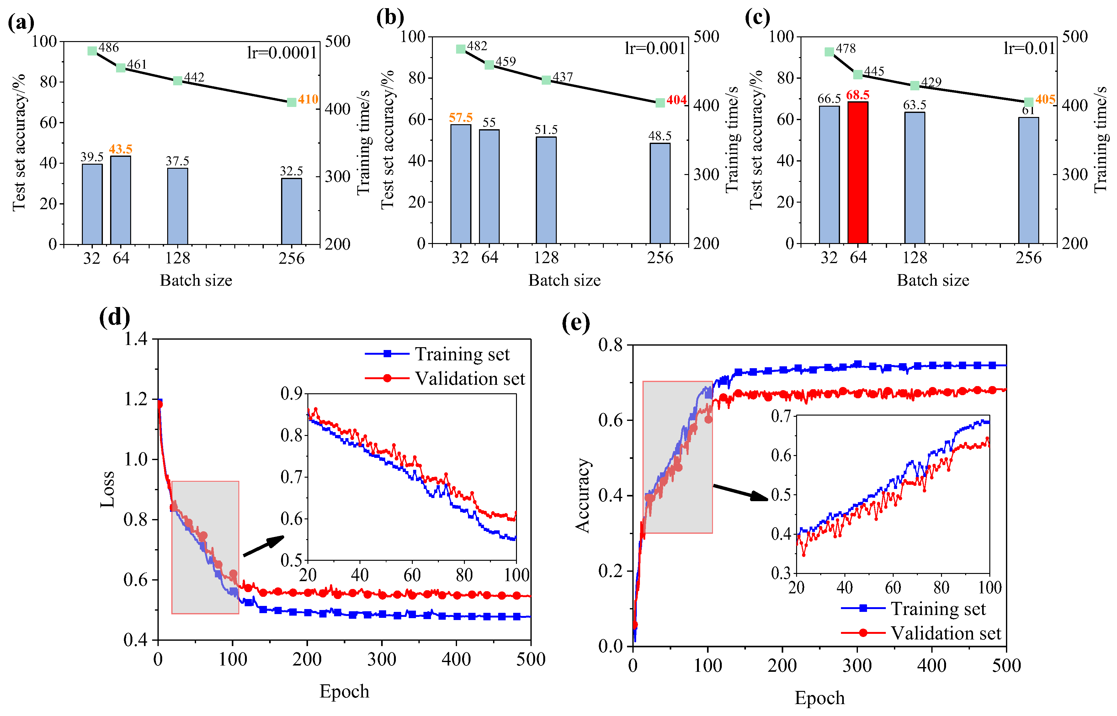
On the basis of three recognition models, experiment results with different learning rates (lr) and sample batches (batch) were recorded. Figure 12 shows the final experiment result of the LeNet-5 model. Figure 12a–c shows the training time and recognition accuracy of the model on the test set under three learning rates (lr = 0.0001, lr = 0.001, and lr = 0.01) and four sample batches (batch = 32, batch = 64, batch = 128, and batch = 256), respectively. The experiment results indicated that the model had the shortest training time of 404 s with lr = 0.001 and batch = 256, but the recognition accuracy of the model on the test set was too low at only 48.5%. When the recognition accuracy of the model reached the highest at 68.5% with lr = 0.01 and batch = 64, its training time was 445 s. In the process of off-line training, if the training time was not much different, so only the recognition accuracy of the test set was regarded as the evaluation standard. The training process of the model with the highest recognition accuracy of 68.5% is shown in Figure 12d,e. The error loss of the training set was slightly lower than the error loss of the validation set during the entire training process, converging to 0.48 and 0.55, respectively. The overall accuracy of the training set was slightly higher than that of the validation set, finally the accuracy reaching 0.75 and 0.68, respectively, thus indicating that the training and learning process of the model was correct and that the model had a certain generalization ability. However, the recognition accuracy of the model could not meet the requirements of practical applications. Further experiments with adjustments of the parameters, such as lr and batch, were carried out, but the final recognition accuracy could not exceed 70%, which indicated that the edge defect recognition model based on LeNet-5 was not effective. To further improve the recognition accuracy, the model structure must be redesigned and adjusted, and a corresponding experiment must be verified. However, ensuring a high recognition accuracy is difficult because of the rather complicated process.
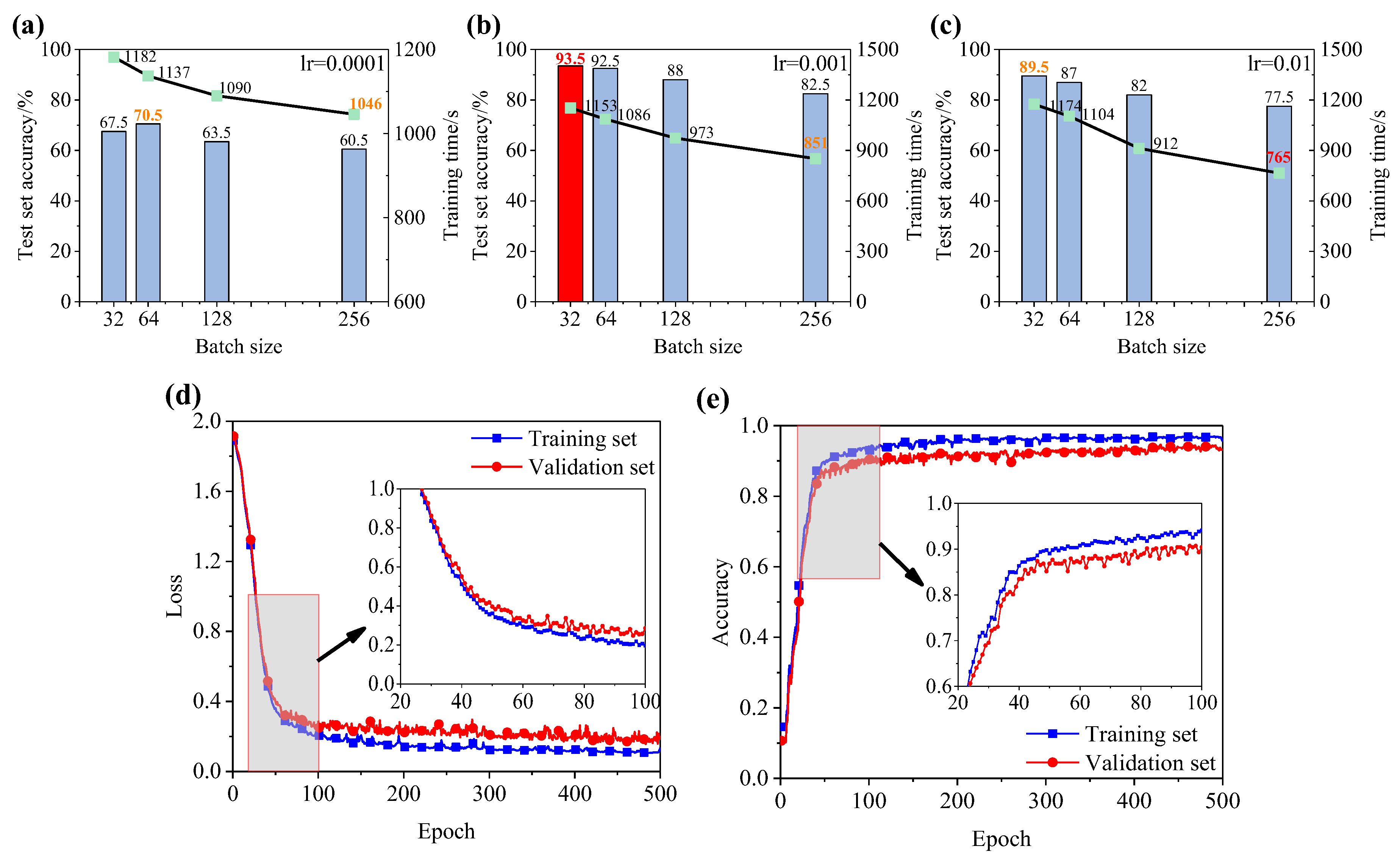
The authors of this paper used the AlexNet convolutional neural network to establish an edge defect recognition model. The experiment results are shown in Figure 13. In Figure 13a–c, two groups with the model’s defect recognition accuracy exceeding 90% on the test set can be observed. When lr = 0.001 and batch = 32 and when lr = 0.001 and batch = 64, the accuracy deviation between the two groups was 1% and the training time deviation was 67 s. Similarly, not considering the training time, the training process of the model with the recognition accuracy of 93.5% is shown in Figure 13d,e. The entire training process was relatively stable, and the error loss of the training set and the validation set converged to 0.11 and 0.19, respectively, which were lower than the error loss of the LeNet-5 recognition model. The accuracy of the training set and the validation set reached 0.96 and 0.93, respectively, which were significantly higher than the accuracy of the LeNet-5 recognition model.
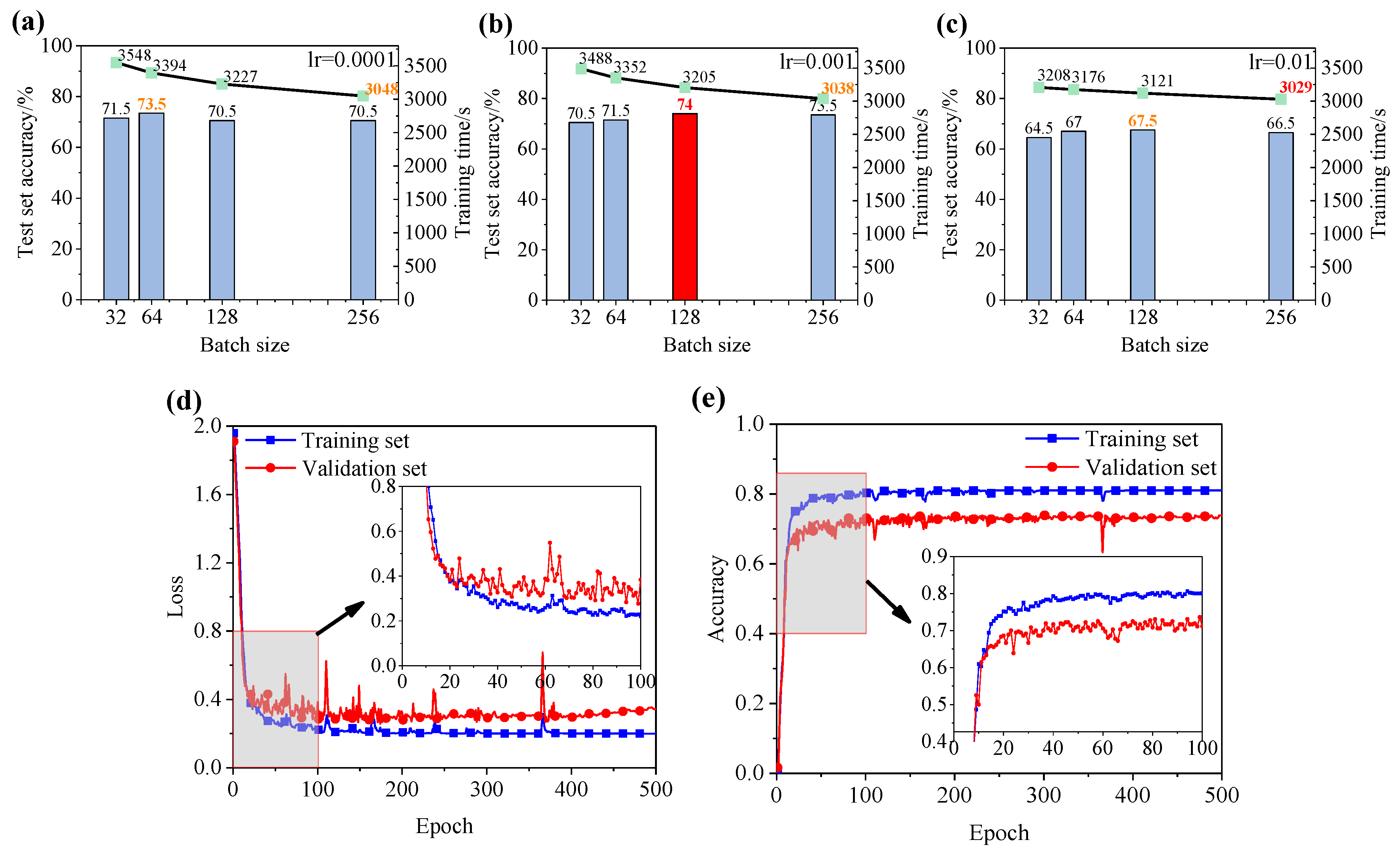
This paper further used the VggNet-16 convolutional neural network to establish an edge defect recognition model. The experiment results are shown in Figure 14. Figure 14a–c shows that when lr = 0.001 and batch = 128, the defect recognition accuracy of the model on the test set was up to 74% and the training time was 3205 s. Figure 14d,e shows that local oscillations existed during the model training process. Meanwhile, when the number of iterations exceeded 400, the error loss of the validation set had an upward trend, indicating that the model had a certain degree of overfitting.
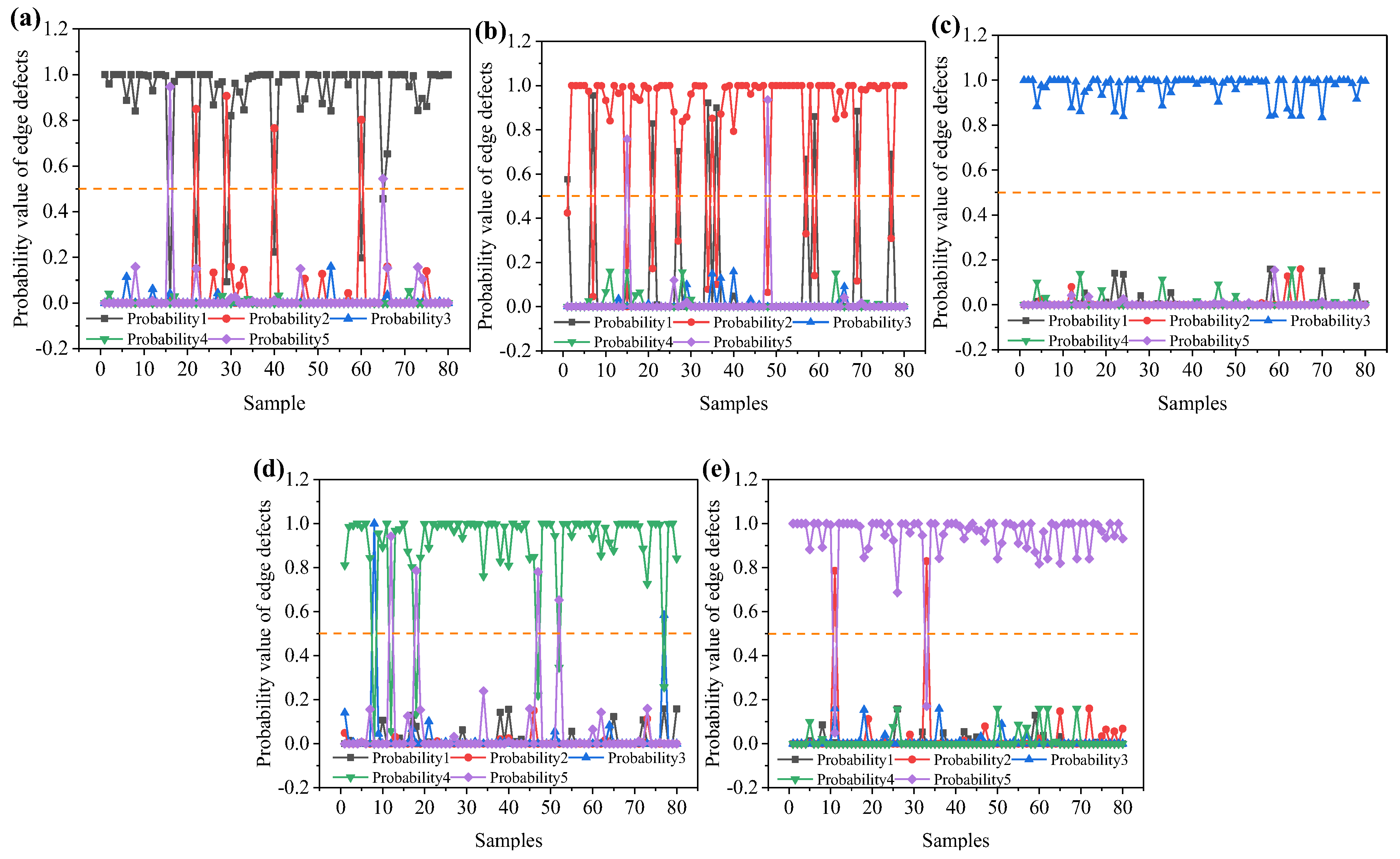
By comparing Figure 12, Figure 13 and Figure 14, it can be seen that the training time of the model slightly decreased with the increase in learning rate and greatly decreased with the increase in sample batch, though too large a batch greatly reduced the recognition accuracy of the model. The defect image recognition time is more important to satisfy online applications. In this paper, the recognition experiment of a single edge defect image was conducted for each model with different parameters. The experiment results are shown in Table 3. The results showed that the average single defect recognition times of three types of CNN models were 2.7, 3.5, and 5.4 ms, respectively. The learning rate and sample batch had no obvious influence on the recognition time of a single defect image. In this paper, the AlexNet (lr = 0.001 and batch = 32) model was selected as the hot rolling strip edge defect recognition model because its accuracy and speed of recognition meet the engineering requirements. Figure 15 shows the visualization recognition results of the model on the test set. The recognition results of the defect image were expressed by the probability value. In Figure 15a–e, the recognition result of each image defect classification is expressed by a probability vector (probability 1, probability 2, probability 3, probability 4, and probability 5). The values of probability 1, probability 2, probability 3, probability 4, and probability 5 represented the scores of five defect classifications (upwarp, black line, crack, slag inclusion, and gas hole, respectively), and the sum of the five probability values was 1. In the process of defect image recognition, when the probability value of a certain item in the probability vector exceeded 0.5 (orange boundary in the figure), the classification of the defect of the image was determined. The recognition performance of edge cracks was the best, and no recognition error was recorded. More errors appeared between the upwarp and black line, which also confirmed the conclusion that the two types defect have the same generation mechanism [27,28]. The confusion matrix of the defect recognition results on the test set is shown in Table 4. According to the diagonal value in this matrix, it can be seen that the model had a better overall recognition and classification effect on edge defects. Based on the value distribution on both sides of the diagonal line, it could also be seen that the upwarp and black line easily caused recognition errors, which had a greater impact on the accuracy of the model. Though a small number of recognition errors were observed between slag inclusion and gas hole, the overall recognition accuracy could meet the requirements of practical application. In the future, in order to further improve and optimize the model, the dataset needs to be expanded and processed, especially to expand the defect images of upwarp, black line, and gas hole as much as possible. Meanwhile, an image-enhancing technique can be introduced to optimize the model.
4. Conclusions
The edge defects of hot rolling strips have five types: upwarp, black line, crack, slag inclusion, and gas hole. The appearance morphologies of these five types of defects show a certain linear feature. However, the width, length, and color of the lines are not completely consistent with the specific texture features. To improve the detection accuracy of edge defects, edge defect recognition models were established on the basis of LeNet-5, AlexNet, and VggNet-16 by using a convolutional neural network as the core.
The edge defect recognition model based on the LeNet-5 convolutional neural network was found to have the highest accuracy of 68.5% on the test set, and its average recognition time for a single defect image was 2.7 ms. Though the model was found to have a certain generalization ability, its prediction accuracy is a bit low. The edge defect recognition model based on the VggNet-16 convolutional neural network had the highest accuracy of 74% on the test set, and its average recognition time for a single defect image was 5.4 ms. The model was found to have local oscillations and a certain overfitting trend during the training process. The edge defect recognition model based on the AlexNet convolutional neural network had the highest accuracy of 93.5% on the test set, and its average recognition time for a single defect image was 3.5 ms.
Among the three models, the edge defect recognition model based on the AlexNet convolutional neural network was found to have the highest prediction accuracy, a good generalization ability, and the best comprehensiveness. However, the accuracy of the model needs to be further improved, especially because the two defects of upwarp and black line are still easily confused. In future research, we plan to adapt some advanced neural networks (such as EfficientNet, EfficientDet, and RegNet) to further improve model performance (accuracy, training speed, recognition speed, transfer ability, etc.). At the same time, more defect images will be collected for model training and testing.
Author Contributions
Conceptualization, D.W.; methodology, D.W. and Y.X.; writing—original draft preparation, D.W. and Y.X.; writing—review and editing, Y.X., B.D., and Y.W.; supervision, H.Y. and M.S.; funding acquisition, D.W. and H.L. All authors have read and agreed to the published version of the manuscript.
Funding
This work was supported by the National Natural Science foundation of China (Grant No. 52074242), and the Natural Science Foundation of Hebei Province, China (Grant No. E2016203482).
Institutional Review Board Statement
Not applicable.
Informed Consent Statement
Not applicable.
Data Availability Statement
Restrictions apply to the availability of these data. Data was obtained from Maanshan Iron & Steel Company Limited and are available from the authors with the permission of Maanshan Iron & Steel Company Limited.
Conflicts of Interest
The authors declare no conflict of interest.
References
- Wang, N.N.; Hou, B.; Song, H.C.; Zhou, L.L.; Liu, Y.X.; Wang, R. Research on the quality online control technology for hot rolled strip. Steel Roll. 2017, 34, 59. [Google Scholar]
- Song, J. Analysis on The Surface Defects of Hot Strips Based on Data Mining Methods. Master’s Thesis, Shanghai Jiao Tong University, Shanghai, China, 2008. [Google Scholar]
- Wu, P.C.; Lu, T.J.; Wang, Y. Development and perspective of automatic strip surface inspection system. Iron Steel 2000, 35, 70. [Google Scholar]
- Ai, Y.H.; Xu, K. Development and prospect of on-line surface inspection of steel plates. Met. World 2010, 5, 37–39. [Google Scholar]
- Xiao, S.H.; Wu, L.; He, W.; Peng, Y. Application of deep learning in surface quality detection. Mach. Des. Manuf. 2020, 1, 288. [Google Scholar]
- Xu, K.; Yang, C.L.; Zhou, P. Technology of on-line surface inspection for Hot rolling Steel Strips and Its Industrial Application. J. Mech. Eng. 2009, 45, 111. [Google Scholar] [CrossRef]
- Wang, C.M.; Zhou, D.D.; Xu, K.; Zhang, H.N. Review of intelligent manufacturing technology in steel industry. Chin. Met. 2018, 28, 1. [Google Scholar]
- Xu, K.; Wang, L.; Wang, J.Y. Surface defect recognition of hot rolling steel plate based on tetrolet transform. J. Mech. Eng. 2016, 52, 13. [Google Scholar] [CrossRef]
- He, Y.H.; Miao, R.T.; Chen, Y.; Liang, S.; Fei, J.H. Development and application of the on-line surface inspection system for hot rolling strips based on LED light source. Baosteel Technol. 2011, 3, 1. [Google Scholar]
- Gan, S.F.; Sun, L.; Yang, C.; Liu, G.Y. Application of multi-level image classification system in surface defect detection of cold-rolled silicon strip. Met. Ind. Autom. 2009, 33, 63. [Google Scholar]
- Yi, Z.H.A.O. Application of deep learning in defects identification of silicon steel sheet. Digit. Technol. Appl. 2017, 12, 19. [Google Scholar]
- Han, Y.L.; Yan, Y.H. Discernment and classification of banding strip surface defect based on BP neural network. Chin. J. Sci. Instrum. 2006, 27, 1692. [Google Scholar]
- Chu, M.X. Research of Key Technologies for Steel Plate Surface Defects Detection. Ph.D. Thesis, Northeastern University, Shenyang, China, 2014. [Google Scholar]
- Xing, J.F. Surface Defect Recognition and System Development of Hot Rolling Strip Based on Convolutional Neural Network. Master’s Thesis, Northeastern University, Shenyang, China, 2019. [Google Scholar]
- Song, K.C.; Yan, Y.H. A noise robust method based on completed local binary patterns for hot rolling steel strip surface defects. Appl. Surf. Sci. 2013, 285, 858. [Google Scholar] [CrossRef]
- Hu, L.T. Research on Surface Defect Recognition of Steel Plate Based on Machine Vision. Master’s Thesis, Wuhan University of Science and Technology, Wuhan, China, 2018. [Google Scholar]
- Xie, F. Research on Surface Defect Detection Technology Based on Machine Vision. Master’s Thesis, Nanjing University of Aeronautics and Astronautics, Nanjing, China, 2019. [Google Scholar]
- Wen, C.; Gao, Y.P.; Gao, L.; Li, X.Y. A new ensemble approach based on deep convolutional neural networks for steel surface defect classification. Procedia CIRP 2018, 72, 1069. [Google Scholar]
- Gao, Y.P.; Gao, L.; Li, X.Y.; Yan, X.G. A semi-supervised convolutional neural network-based method for steel surface defect recognition. Robot. Comput. Integr. Manuf. 2020, 61, 101825. [Google Scholar] [CrossRef]
- Saiz, F.A.; Serrano, I.; Barandiáran, I.; Sánchez, J.R. A robust and fast deep learning-based method for defect classification in steel surfaces. In Proceedings of the 2018 International Conference on Intelligent Systems (IS), Funchal-Madeira, Portugal, 25–27 September 2018; pp. 455–460. [Google Scholar]
- Lee, S.Y.; Tama, B.A.; Moon, S.J.; Lee, S. Steel surface defect diagnostics using deep convolutional neural network and class activation map. Appl. Sci. 2019, 9, 5449. [Google Scholar] [CrossRef] [Green Version]
- He, Y.; Song, K.C.; Dong, H.W.; Yan, Y.H. Semi-supervised defect classification of steel surface based on multi-training and generative adversarial network. Opt. Lasers Eng. 2019, 122, 294. [Google Scholar] [CrossRef]
- He, Y.; Song, K.C.; Meng, Q.G.; Yan, Y.H. An end-to-end steel surface defect detection approach via fusing multiple hierarchical features. IEEE Trans. Instrum. Meas. 2020, 69, 1493–1504. [Google Scholar] [CrossRef]
- Dong, H.W.; Song, K.C.; He, Y.; Xu, J.; Yan, Y.H.; Meng, Q.G. PGA-net: Pyramid feature fusion and global context attention network for automated surface defect detection. IEEE Trans. Ind. Inform. 2019, 16, 7448–7458. [Google Scholar] [CrossRef]
- Guan, S.Q.; Lei, M.; Lu, H. A Steel Surface Defect Recognition algorithm based on improved deep learning network model using feature visualization and quality evaluation. IEEE Access 2020, 8, 49885. [Google Scholar] [CrossRef]
- Fu, G.Z.; Sun, P.Z.; Zhu, W.B.; Yang, J.X.; Gao, Y.L.; Yang, M.Y.; Gao, Y.P. A deep-learning-based approach for fast and robust steel surface defects classification. Opt. Lasers Eng. 2019, 121, 397. [Google Scholar] [CrossRef]
- You, H.C.; Wang, D.C.; Gao, T.; Wang, H.B.; Zhang, W. Formulation mechanism of edge seam defects for hot rolling IF steel. Heavy Mach. 2019, 6, 16. [Google Scholar]
- Hu, X.W.; Wang, D.C.; Gao, T.; You, H.C.; Zhao, H. Treatment measures of edge seam defects for hot rolling IF steel. Heavy Mach. 2020, 1, 53. [Google Scholar]
- Chun, P.J.; Yamane, T.; Izumi, S.; Kameda, T. Evaluation of tensile performance of steel members by analysis of corroded steel surface using deep learning. Metals 2019, 9, 1259. [Google Scholar] [CrossRef] [Green Version]
- Kim, M.; Han, J.C.; Hyun, S.H.; Janssens, O.; Van Hoecke, S.; Kee, C.; De Neve, W. Medinoid: Computer-aided diagnosis and localization of glaucoma using deep learning. Appl. Sci. 2019, 9, 3064. [Google Scholar] [CrossRef] [Green Version]
- Huang, J.; Zhang, G. Survey of object detection algorithms for deep convolutional neural networks. Comput. Eng. Appl. 2020, 56, 12. [Google Scholar]
- Javaheri, E.; Kumala, V.; Javaheri, A.; Rawassizadeh, R.; Lubritz, J.; Graf, B.; Rethmeier, M. Quantifying mechanical properties of automotive steels with deep learning based computer vision algorithms. Metals 2020, 10, 163. [Google Scholar] [CrossRef] [Green Version]
- Kesse, M.A.; Buah, E.; Handroos, H.; Ayetor, G.K. Development of an artificial intelligence powered TIG welding algorithm for the prediction of bead geometry for TIG welding processes using hybrid deep learning. Metals 2020, 10, 451. [Google Scholar] [CrossRef] [Green Version]
- Lecun, Y.; Bottou, L.; Bengio, Y.; Haffner, P. Gradient-based learning applied to document recognition. Proc. IEEE 1998, 86, 2278. [Google Scholar] [CrossRef] [Green Version]
- Krizhevsky, A.; Sutskever, I.; Hinton, G.E. ImageNet Classification with deep convolutional neural networks. Commun. ACM 2012, 1, 84–90. [Google Scholar] [CrossRef]
- Simonyan, K.; Zisserman, A. Very deep convolutional networks for large-scale image recognition. arXiv 2014, arXiv:1409.1556. [Google Scholar]
Figure 1.
Relationship between the edge defect image set and the perfect image set.

Figure 2.
Edge defect detection of a hot rolling strip.

Figure 3.
Evolution process of edge defects.

Figure 4.
Typical surface defects of a hot rolling strip.

Figure 5.
Structure of the CNN recognition model for hot rolling strip edge defect.

Figure 6.
Convolution operation process.

Figure 7.
Several typical activation function images: (a) sigmoid, (b) tanh, (c) relu, and (d) prelu.
Figure 7.
Several typical activation function images: (a) sigmoid, (b) tanh, (c) relu, and (d) prelu.

Figure 8.
Two pooling methods: (a) average-pooling and (b) max-pooling.

Figure 9.
Basic process of convolutional neural networks.

Figure 10.
Edge defect dataset of a hot rolling strip.

Figure 11.
Three CNN recognition models for edge defects: (a) LeNet-5, (b) AlexNet, and (c) VggNet-16.
Figure 11.
Three CNN recognition models for edge defects: (a) LeNet-5, (b) AlexNet, and (c) VggNet-16.

Figure 12.
Edge defect LeNet-5 CNN model experiment results: (a) test set accuracy and training time with lr = 0.0001, (b) test set accuracy and training time with lr = 0.001, (c) test set accuracy and training time with lr = 0.01, (d) error loss of training process with lr = 0.01 and batch = 64, and (e) accuracy of training process with lr = 0.01 and batch = 64.

Figure 13.
Edge defect AlexNet CNN model experiment results: (a) test set accuracy and training time with lr = 0.0001, (b) test set accuracy and training time with lr = 0.001, (c) test set accuracy and training time with lr = 0.01, (d) error loss of training process with lr = 0.001 and batch = 32, and (e) accuracy of training process with lr = 0.001 and batch = 32.

Figure 14.
Edge defect VggNet-16 CNN model experiment results: (a) test set accuracy and training time with lr = 0.0001, (b) test set accuracy set and training time with lr = 0.001, (c) test set accuracy and training time with lr = 0.01, (d) error loss of training process with lr = 0.001 and batch = 128, and (e) accuracy of training process with lr = 0.001 and batch = 128.

Figure 15.
Visualization results of five types of edge defect recognition on the test set: (a) upwarp, (b) black line, (c) crack, (d) slag inclusion, and (e) gas hole.
Figure 15.
Visualization results of five types of edge defect recognition on the test set: (a) upwarp, (b) black line, (c) crack, (d) slag inclusion, and (e) gas hole.


Table 1.
Morphological features of edge defects. SQDS: surface quality detection system.
| Feature | Upwarp | Black Line | Crack | Slag Inclusion | Gas Hole |
|---|---|---|---|---|---|
| Length | Continuous or discontinuous with different lengths. | Continuous or discontinuous with different lengths. | 20~100 mm | 100~1000 mm | 150~500 mm |
| Width | 1~3 mm | <1 mm | 5~20 mm | 2~5 mm | 1~5 mm |
| Shape | A straight and uniform-width line accompanied with upwarp. | A straight and uniform-width line. | Branch. | strip with uniformwidth. | strip with texture. |
| Morphology (Physical) |  |  |  |  |  |
| Morphology (SQDS) |  |  |  |  |  |
Table 2.
Image distribution of each part in the training set, the validation set, and the test set.
| Dataset | Upwarp | Black Line | Crack | Slag Inclusion | Gas Hole | Aggregate |
|---|---|---|---|---|---|---|
| Training set | 240 | 240 | 240 | 240 | 240 | 1200 |
| Validation set | 80 | 80 | 80 | 80 | 80 | 400 |
| Test set | 80 | 80 | 80 | 80 | 80 | 400 |
| Aggregate | 400 | 400 | 400 | 400 | 400 | 2000 |
Table 3.
Recognition time of a single defect image on the test set with different models (ms).
| Batch | LeNet-5 | AlexNet | VggNet-16 | ||||||
|---|---|---|---|---|---|---|---|---|---|
| Lr = 0.0001 | Lr = 0.001 | lr = 0.01 | lr = 0.0001 | lr = 0.001 | lr = 0.01 | lr = 0.0001 | lr = 0.001 | lr = 0.01 | |
| 32 | 2.386 | 2.381 | 2.386 | 3.462 | 3.462 | 3.395 | 5.131 | 5.737 | 5.508 |
| 64 | 2.514 | 2.572 | 2.568 | 3.513 | 3.479 | 3.401 | 5.305 | 5.542 | 5.416 |
| 128 | 2.844 | 2.825 | 2.859 | 3.566 | 3.783 | 3.495 | 5.324 | 5.493 | 5.703 |
| 256 | 3.180 | 3.081 | 3.081 | 3.799 | 3.544 | 3.385 | 5.280 | 5.427 | 5.464 |
Table 4.
Confusion matrix of the edge defect recognition model on the test set.
| Confusion Matrix | Model Classification | |||||
|---|---|---|---|---|---|---|
| Upwarp | Black Line | Crack | Slag Inclusion | Gas Hole | ||
| Actual classification | Upwarp | 74 | 4 | 0 | 0 | 2 |
| Black line | 10 | 68 | 0 | 0 | 2 | |
| Crack | 0 | 0 | 80 | 0 | 0 | |
| Slag inclusion | 0 | 0 | 2 | 74 | 4 | |
| Gas hole | 0 | 2 | 0 | 0 | 78 | |
Publisher’s Note: MDPI stays neutral with regard to jurisdictional claims in published maps and institutional affiliations. |
© 2021 by the authors. Licensee MDPI, Basel, Switzerland. This article is an open access article distributed under the terms and conditions of the Creative Commons Attribution (CC BY) license (http://creativecommons.org/licenses/by/4.0/).
Share and Cite
MDPI and ACS Style
Wang, D.; Xu, Y.; Duan, B.; Wang, Y.; Song, M.; Yu, H.; Liu, H. Intelligent Recognition Model of Hot Rolling Strip Edge Defects Based on Deep Learning. Metals 2021, 11, 223. https://0-doi-org.brum.beds.ac.uk/10.3390/met11020223
AMA Style
Wang D, Xu Y, Duan B, Wang Y, Song M, Yu H, Liu H. Intelligent Recognition Model of Hot Rolling Strip Edge Defects Based on Deep Learning. Metals. 2021; 11(2):223. https://0-doi-org.brum.beds.ac.uk/10.3390/met11020223
Chicago/Turabian StyleWang, Dongcheng, Yanghuan Xu, Bowei Duan, Yongmei Wang, Mingming Song, Huaxin Yu, and Hongmin Liu. 2021. "Intelligent Recognition Model of Hot Rolling Strip Edge Defects Based on Deep Learning" Metals 11, no. 2: 223. https://0-doi-org.brum.beds.ac.uk/10.3390/met11020223
Note that from the first issue of 2016, this journal uses article numbers instead of page numbers. See further details here.