A Review of the Boiling Curve with Reference to Steel Quenching

1
Facultad de Ciencias Químicas, Universidad Autónoma de Coahuila, Saltillo 25280, Mexico
2
Universidad Politécnica de la Región Ribereña, Cd. Miguel Alemán 88300, Mexico
3
Centro de Investigación y de Estudios Avanzados del I.P.N., Unidad Saltillo, Industria Metalúrgica # 1062, Parque Industrial Saltillo-Ramos Arizpe, Ramos Arizpe 25900, Mexico
*
Author to whom correspondence should be addressed.
Metals 2021, 11(6), 974; https://0-doi-org.brum.beds.ac.uk/10.3390/met11060974
Submission received: 9 May 2021
/
Revised: 30 May 2021
/
Accepted: 2 June 2021
/
Published: 17 June 2021
(This article belongs to the Special Issue Heat Treatment of Steels)
Abstract
:This review presents an analysis and discussion about heat transfer phenomena during quenching solid steel from high temperatures. It is shown a description of the boiling curve and the most used methods to characterize heat transfer when using liquid quenchants. The present work points out and criticizes important aspects that are frequently poorly attended in the technical literature about determination and use of the boiling curve and/or the respective heat transfer coefficient for modeling solid phase transformations in metals. Points to review include: effect of initial workpiece temperature on the boiling curve, fluid velocity specification to correlate with heat flux, and the importance of coupling between heat conduction in the workpiece and convection boiling to determine the wall heat flux. Finally, research opportunities in this field are suggested to improve current knowledge and extend quenching modeling accuracy to complex workpieces.
1. Introduction
Historically, steel heat treatment has evolved from being an ancestral craft to a sophisticated technology that responds to a higher demand of a wide variety of products with increasingly strict quality standards. This technology relies on developments on several knowledge areas like, materials, such as material science, mechanical metallurgy, heat transfer, computation, instrumentation and control theory, robotics, etc. Nonetheless, the core knowledge is represented by the relationship between processing conditions during heat treatment, and microstructure and properties of the workpiece that are obtained after treatment. Of course, processing conditions always includes a thermal cycle ending with a target cooling rate on the workpiece. This cooling rate is very important to determine the final microstructure, properties and physical integrity of the workpiece.
Mathematical modeling has been used with more frequency in the last three decades to understand and quantitatively predict the previously mentioned relationship between processing-microstructure-properties. Modeling or characterizing experimentally the rate of heat transfer during quenching is the basic step for modeling kinetics of solid-state phase transformation in steels, which in turn is used to predict final microstructure, mechanical properties and workpiece internal stresses and deformations.
The motivation of the present work is to point out and criticize important aspects that are frequently underrepresented in the technical literature about determination and use of the boiling curve and/or the respective heat transfer coefficient for metal quenching modeling. Points to review include: effect of initial workpiece temperature on the boiling curve, modification of temperatures that narrow down boiling regimes, uniformity and magnitude of heat flux in production heat treatment, and the effect of the workpiece size and metal properties on the boiling curve. This article summarizes an overview of basic steel quenching concepts, followed by the presentation and analysis of the established theory of heat transfer phenomena during quenching using a vaporizable liquid.
Two classical handbooks on heat treatment and quenching [1,2] were identified as the point to start for this work. In addition, the document reflects opinions emerged from more than 20 years of professional experience (FAAG), in production line, laboratory and computer modeling, on heat transfer in continuous casting of steel. Recent advances on steel quenching have been also reviewed in the context of the present analysis and discussion.
2. Steel Heat Treating Concepts
Heat treatment of alloys or metals is a term to include any thermal cycle from heating a workpiece to a solubilization temperature in the solid state, soaking the workpiece at this temperature to achieve the target solubilization level, and then cooling it down fast enough to develop the metal microstructure that grants the aimed mechanical properties and physical integrity of the workpiece. Solubilization temperature is a function of the chemical composition of the treated alloy; for example, for steels, it is generally from 800 to 950 °C, depending on the steel grade. This temperature is above the eutectoid temperature at which the ferrite phase (Fea, Body-Centered Cubic structure) and cementite (Fe3C) transform into austenite phase (Feg, Face-Centered Cubic structure). Because of its crystal structure, austenite is able to dissolve the carbon released from the decomposition of the cementite. Other examples of heat treatable alloys include specific grades of aluminum, titanium and copper alloys. Solubilization temperatures may be estimated from a binary phase diagram. However, since alloys contain several elements, sometimes pseudo-binary phase diagrams or, if available, ternary phase diagrams are preferred.
The cooling rate of the workpiece plays a major role to determine the microstructure and mechanical properties of the alloys. For example, austenite is generally quenched to obtain martensite phase (Fea’, Body-Centered Tetragonal structure). The cooling rate should be high enough to “freeze” the dissolved carbon avoiding its precipitation after cooling. Indeed, martensite is a carbon-supersaturated solid solution, therefore is a non-equilibrium phase which of course does not appear in any equilibrium diagram. Martensite formation is graphically represented by a Temperature-Time-Transformation (TTT) diagram or by a Continuous Cooling Transformation (CCT) diagram. The former represents isothermal transformations, i.e., the workpiece is cooled down at “infinite velocity” from the solubilization temperature to the transformation temperature. Then, it is hold at this temperature until the solid phase transformation ends. On the other hand, CCT diagrams represent what actually happens during cooling at a constant rate. The alloy structure transforms at inconstant temperature. Both diagrams, TTT and CCT, represent time-temperature maps to locate every phase that would form. For example, when steel cools down at a low rate, it will form the equilibrium phases, ferrite and cementite. However, if the cooling rate is higher, bainite may form. This is a mixture of nonlamellar aggregate of carbides and plate-shaped ferrite. If the cooling rate is even higher, the austenite will start to transform to martensite at temperature Ms. As the sample cools down, an increasingly percentage of austenite transforms to martensite until reaching the temperature, Mf, at which the transformation is completed. The values of hardness and tensile strength for this phase are well above than those obtained for bainite or ferrite phases. Hardenability refers to the steel’s capability to form martensite. The higher the hardenability of a steel, the easier it would be to form martensite since the required minimum cooling rate would be less demanding.
This review is focused on heat transfer phenomena during solid metal quenching, when using liquids as quenchant media. Water, polymer aqueous solutions, and mineral oils are generally used for quenching metals. The choice for a quenching medium for a specific application is based on the required cooling rate, according to the CCT diagram, to form the target phases, but avoiding quality issues like piecework fracture, unacceptable distortion or dimensional variation which would result from thermal and phase transformation stresses. To achieve this, the latent heat and temperature of vaporization, surface tension, and viscosity are the main liquid properties to take into consideration when choosing a quenching medium. Finally, the fluid flow velocity passing over the workpiece determines the rate of heat transfer and therefore has a major impact on the cooling rate.
3. Boiling and Quenching Heat Transfer
This document is focused on quenching workpieces which initial temperature is well above the boiling temperature of the quenching liquid, for example 800 °C. The boiling curve is a convenient graphic representation of the heat flux removed from the workpiece surface, or wall surface, as a function of its temperature, Tw. The heat flux is defined as the heat flow removed per unit surface area of the workpiece, q (W/m2), and therefore it is a local quantity, i.e., it may change along the surface of the workpiece. Differently from gas quenching, liquid quenching includes boiling phenomenon which leads to a parabolic type-function dependence of q with Tw. Such behavior is not obtained from gas quenching, since for this case heat flow is maximum at the beginning of cooling and then decreases exponentially with time. Boiling curves are obtained under natural convection flow (pool boiling) or forced convection flow. Both types of flow are applicable to quenching operations. Furthermore, boiling curves can be determined under steady or transient temperature conditions. In the former method, a specimen is heated by a controlled heat source while simultaneously a quenchant flow removes heat from the specimen to reach an equilibrium temperature. This case is mainly found when quenching using sprays, see for example references [3,4,5,6]. Abbasi et al. [3] used an electric resistance to supply heat to a metallic sample that simultaneously received a water spray to reach an equilibrium temperature. The authors studied the effect of spray pressure on the removed heat transfer and found that it increases the rate of heat transfer. They attributed this result to an increase in the droplet velocity with spray pressure. Araki et al. [4] also used another arrangement of electrical resistances to supply heat to a thin metal disk which received a controlled spray of water droplets. The disk was heated up to steady temperatures of 240 to 860 °C and received a rate of droplets of 0.5, 1, 2 and 3 droplets per second at velocities between 1.5 to 4 m/s. Bernardin and Mudawar [5] studied film boiling heat transfer of an isolated droplet stream. They also used electric resistances to supply heat to a polished nickel plate to reach equilibrium temperatures up to 400 °C. The authors presented empirical correlations of the heat flux removed by these continuous stream of monodispersed water droplets. All these studies used a low mass flux of droplets impacting the surface (<1 kg/m2s), and also the droplets velocities were below 5 m/s. More recently, Hernández-Bocanegra et al. [6] developed a new steady state system which is able to study actual production air-mist and spray jets. It uses electromagnetic heating to supply heat to a platinum sample 8 mm diameter by 2.5 mm thickness. Using a properly designed coil, a 5 kW high frequency generator was able to maintain the sample at equilibrium temperatures ranging from 200 to 1200 °C while simultaneously receiving a high mass flux spray. Droplets impacted the platinum disk at velocities between 10 and 30 m/s, which represents high pressure spray quenching conditions. On the other hand, transient temperature experiments consist in preheating an instrumented specimen in a muffle and then transporting it to a quenching rig to generate the corresponding cooling curve until ambient temperature. Reference [7] details a concept on thermal equilibrium establishment which is useful to determine the required soaking (heating) time for the workpiece to reach the target austenitization temperature, and references [8,9] describe some examples of experimental cooling curves. Kobasko [7] proposed a universal correlation to calculate the heating (soaking) time of any steel part. This time is directly proportional to Kondratjev form factor, K, is inversely proportional to thermal diffusivity of a material and Kondratjev number, Kn, and depends on the accuracy of the temperature measurement. Reference [1] (pp. 69–128) describes the technique to measure cooling curves for steel quenching characterization. Several standard probes, instrumented with thermocouples, have been developed to obtain such curves. Some of them are the SAE 5145 steel Grossmann probe, French probe, Beck hollow spherical copper probe, spherical silver probe, JIS silver probe, and Liscic-NANMAC steel probe. This method has been also applied to study secondary cooling of continuous casting strands. Stewart et al. [8] implemented a test apparatus using a stainless-steel specimen cooled from 1200 °C to ambient temperature. Li et al. [9] also used an instrumented stainless-steel plate to obtain cooling curves from several initial temperatures, 400, 550, 700, 800, 900 and 1000 °C. They found that the respective boiling curves depend on the initial temperature. This document focuses on the boiling curve obtained under transient temperature conditions.
3.1. Boiling Curve Determination
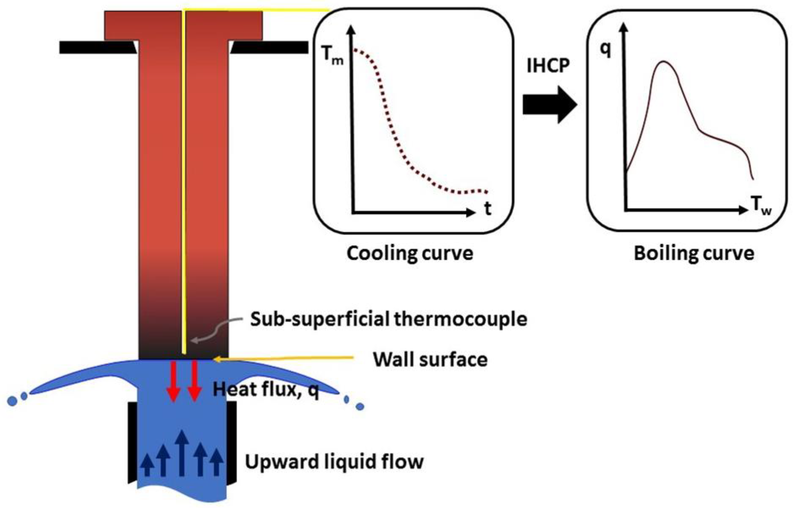
Boiling curves are obtained from thermal analysis. This is an experimental technique which uses embedded sub-superficial thermocouples within the workpiece, as it is shown in Figure 1. A typical distance from wall surface to thermocouple tip is 1 to 3 mm. The temperature-time data recorded during quenching are used to solve the so-called Inverse Heat Conduction Problem (IHCP) [10]. This method solves iteratively the heat conduction differential equation to find the proper boundary condition consisting in the heat flux evolution function q(t) that minimizes the sum of absolute differences between the measured, Tm, and computed, Tc, temperatures, , where N is the number of data points collected during the quenching test. The computed temperatures correspond to the thermocouple tip position at the recorded times during cooling. The final solution of the heat conduction equation also provides the temperature evolution at any location within the solid, in particular it provides the temperature at the wall surface, Tw. Therefore, the solution of the IHCP leads to the q vs. Tw plot. Sometimes, the wall temperature is replaced by the wall superheat defined by the difference Tw − Tsat, where Tsat is the saturation temperature of the liquid, i.e., its boiling temperature. The boiling curve would be the same, except for the shift of the temperature scale. Figure 1 shows a graphic summary of the boiling curve determination from thermal analysis using the solution of the IHCP.
3.2. Effect of Initial Temperature of the Solid Workpiece
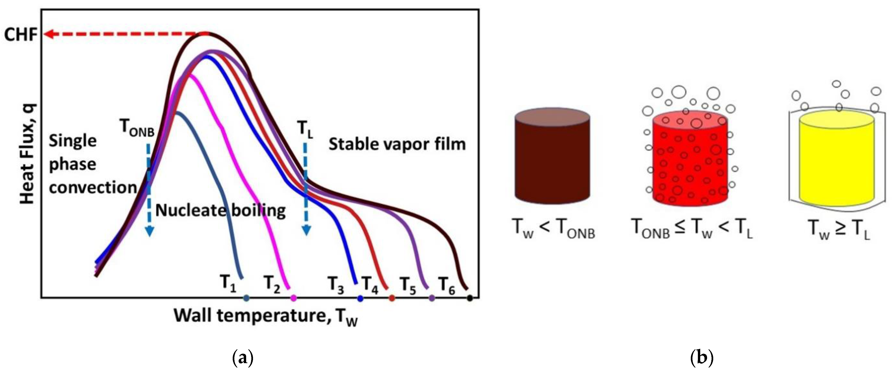
Figure 2a shows typical boiling curves when quenching metallic workpieces from several initial temperatures, T1, T2, …, and T6. As it was mentioned previously, reference [9] presents an example using several initial temperatures between 400 to 1000 °C and quenching stainless-steel plates using a water spray. At any initial temperature, the heat flux is low but increases as the surface temperature decreases until reaching a maximum value, so called critical heat flux (CHF). Thereafter, heat flux keeps decreasing during cooling. At this point, it is convenient to say that Babu et al. [11] proposed a normalized boiling curve to represent all curves for different soaking temperatures into a single curve. In spite of its usefulness, this method has not gained further visibility in the research community. Figure 2b shows schematically the boiling phenomena occurring on the surface of a workpiece during its quenching by immersion. They are described as follows: At higher initial temperatures, a continuous vapor film forms on the solid surface, which acts as a thermal resistance for heat flow. The presence of this vapor blanket explains the quasi-plateaus observed in the curves corresponding to initial temperatures, Tw ≥ T3. Heat flux is kept at a relatively low value; however, when the temperature drops, the vapor film collapses under the liquid pressure, and heat flux increases as a result of a direct contact between the solid surface and the liquid. However, for the curves with Tw < T3 the plateau does not appear, suggesting the absence of an initial stable vapor film. Leidenfrost temperature, TL, is defined as the minimum wall temperature where the stable vapor film regime prevails. Below this temperature, nucleate boiling regime appears, in which swarms of bubbles continuously form and detach from the wall surface. This process is maintained until wall temperature is too low to promote boiling. This is the onset of nucleate boiling temperature, TONB, and is where single phase convection regime appears. The above explanation does not clarify why heat flux is very low at the starting high temperature. This initial low heat flux has mainly attributed to the measurement delay from the thermocouple (time constant). This is a characteristic delay that depends on the wire diameter, the thinner the wire the shorter the delay. Rabin and Rittel [12] showed that the time response of a solid-embedded thermocouple is far from being similar to the corresponding response of a fluid-immersed thermocouple. The authors found that the solid-embedded thermocouple has a significantly faster time response at the initiation of the process, but it requires a much longer time to reach a steady state temperature. They also claim that the thermal diffusivity of the thermocouple should be at least one order of magnitude higher than that of the measured domain in order to obtain meaningful results in transient measurements. This is difficult to obtain for quenching metals, since both, thermocouple and workpiece have mutually similar thermal diffusivity values.
3.3. Effect of Quenchant Liquid
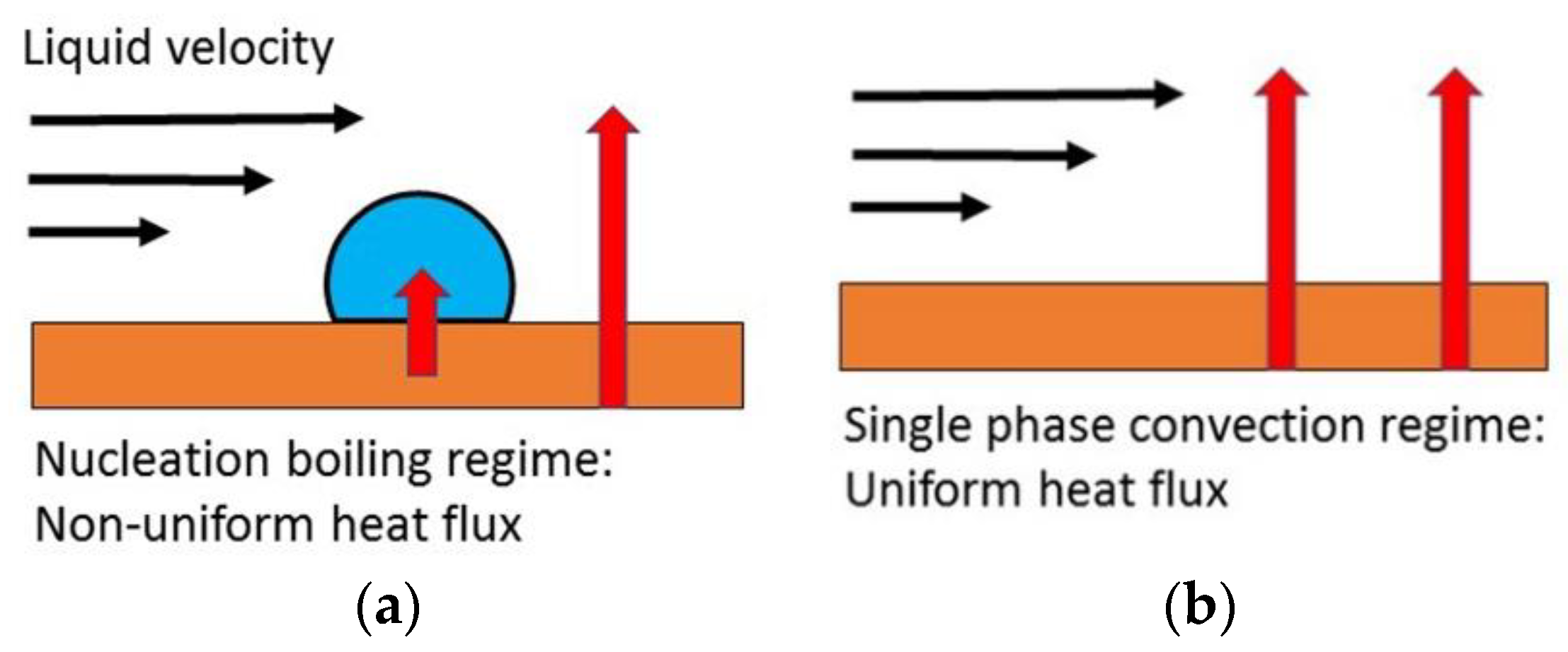
The quenchant liquid properties that have a major impact on the quenching process are: the boiling latent heat and temperature, viscosity, and surface tension. Boiling temperature, also called saturation temperature, Tsat, has an effect on the transition temperature from the nucleate boiling regime to the single-phase convection regime, i.e., over the onset of nucleate boiling temperature, TONB. This temperature is always larger than the saturation temperature, especially when quenching under forced convection. In this case, the flowing liquid spends a very short time in contact with the wall surface, preventing its boiling, even if the wall temperature is many degrees above Tsat. In contrast, for natural convection, TONB exceeds only few degrees the value of Tsat. The wall superheating to reach the nucleate boiling regime, ΔTw = TONB − Tsat, is therefore dependent on the fluid dynamics of the quenchant. This means that under constant fluid flow conditions, a liquid which has a larger value for Tsat will have a larger TONB than the corresponding value for a liquid having a smaller Tsat. This is the case for water and oil, two commonly used quenchants. Water saturation temperature at 1 atm is 100 °C, while the boiling temperature of a typical mineral oil is 280 °C. Therefore, TONB for oil is larger than the corresponding value for water. TONB is particularly important because at wall temperatures above it, vapor bubbles form on the wall surface, creating an obstacle for a direct liquid-solid contact. Vapor thermal conductivity is one order of magnitude smaller than that of liquid. Therefore, the rate of heat conduction through the vapor bubbles is considerably smaller than heat conduction through the liquid. This is represented schematically in Figure 3a,b, where the vertical arrows represent the heat flux from the wall. As a result, heat flux from a wall is more uniform when single phase convection is present, that is, when Tw < TONB. Heat flux uniformity is especially important to minimize thermal and phase transformation stresses. When martensite phase forms during quenching, its higher specific volume with respect to austenite phase generates stresses in the workpiece. Quenching is a controlled cooling process to form martensite as uniform as possible, avoiding that the corresponding stresses may lead to unacceptable workpiece distortion or even crack formation. Martensite forms at a temperature, Ms, that depends on the steel grade. Therefore, it is advisable that TONB > Ms. This is the main reason oil is used as a quenchant rather than water for treating steel grades that are more susceptible to crack formation and distortion during quenching.
The latent heat for vaporization also plays an important role to remove heat during quenching. The higher the latent heat is, the slower the rate of bubble formation becomes. This, in turn, influences the temperature range for each boiling regime to occur.
Liquid viscosity, as defined by Newton’s viscosity law, is a physical property that measures the fluid resistance to flow under a given shear stress. This property determines the velocity profile in the fluid within the boundary layer. This layer is a thin region located just over the wall and it may be formed by liquid, a mixture liquid-vapor, or vapor phase, depending on the present boiling regime. Liquid viscosity has an effect in the single-phase convection and nucleate boiling regimes. A low viscosity value promotes a higher fluid velocity and therefore an improved rate of heat transfer in the single-phase regime. In addition, a low viscosity value favors a faster vapor bubble growth and detachment from the wall; this improves heat flux in the nucleate boiling regime. Generalization of the previous ideas should be taken with caution since liquid viscosity is a strong function of temperature. Viscosity changes during quenching should be considered carefully to properly model the heat transfer process.
Surface tension, , is a property of an interface liquid-gas that measures the energy per unit surface area. The higher the surface tension, the larger is the energy associated with this free surface and the more difficult is to increase it. Surface tension plays a role in the wetting of the wall surface and in the rate of bubble formation and growth. This is discussed below in Section 3.5.
3.4. Effect of Liquid Velocity and Wall Temperature
Before presenting the effect of liquid velocity and wall temperature it is useful to recall the connection between the heat transfer coefficient, h, and the boiling curve, which is given by the Newton convection equation expressed as,
where q is the heat flux at the wall, as defined previously and Tf is the bulk liquid temperature. Therefore, h can be obtained from Equation (1) and using the boiling curve data (q vs. Tw). Readily, we can plot the corresponding h vs. Tw curve. This curve is also a parabolic-type function having a maximum value at a temperature which is generally close to that for the CHF.
Liquid velocity plays an important role in heat transfer from a wall surface to the fluid. The laminar boundary layer theory shows that the local heat flux from a flat wall, at a distance x from the leading edge of the plate, is given by the following equation [13],
where k and v are the thermal conductivity and the kinematic viscosity of the fluid, respectively; Pr is the Prandtl number (=v/α, kinematic viscosity divided by the thermal diffusivity of fluid), and V∞ is the fluid velocity relative to the wall, and Tw is the wall temperature. The term that appears inside the curly brackets represents the local heat transfer coefficient for a single-phase fluid flowing parallel to the wall. Equation (2) shows that heat flux increases with the square root of the fluid velocity. During quenching, the previous equation is only valid under the single-phase convection regime. Nucleate boiling regime introduces bubble formation, growth and detachment from the wall surface and Equation (2) is no longer valid. However, heat flux in this regime also increases with fluid velocity. Finally, the stable vapor blanket regime leads also to a single phase flowing over the wall surface. However, the combined heat flux is the sum of two contributions: a convection contribution given by Equation (2) and a radiation term given by the following equation.
where s = 5.669 × 10⁻⁸ W/m2K4 is the Stefan–Boltzmann constant, F is the view factor which is commonly equal to one for quenching workpieces, and e is the emissivity of the wall surface. Analogous to Equation (2), the term inside the curly brackets represents the radiative heat transfer coefficient. It is seen that this coefficient depends on the wall absolute temperature rised to the third power. Table 1 presents some examples of combined heat transfer coefficients as a function of the fluid velocity [14,15,16]. They were determined from thermal analysis and the solution of the IHCP. Data from refs. [14,16] were obtained using the ivf SmartQuench® system which follows specifications of ISO 9950. It includes an Inconel 600 instrumented probe that is heated up in a resistance furnace to the test initial temperature. Then, the probe is immersed into a preheated oil bath and the cooling curve is registered. Reference [15] reports the use of steel cylindrical probes, (Ø28 mm × 56 mm height and Ø44 mm × 88 mm) to study the effect of both, fluid velocity and probe diameter on the heat flux. The cylinders were thermally isolated in the basal and top surfaces, to force heat to flow in the radial direction. Heat transfer coefficient values were estimated from data of references [14,15] using Equation (1). In all cases, the heat transfer coefficient increases with fluid velocity. The table shows only the peak values for the heat transfer coefficient and misses the detailed variation of h with wall temperature, Tw, and also with the initial temperature, To.
3.5. Effect of Wall Surface Roughness and Wettability
Essentially, wall surface roughness is represented by the average length of mili or micro scale bumps and batches forming a net of gaps over the wall surface. When a workpiece is submerged into a liquid, air remains trapped in these gaps. During the nucleate boiling regime, vapor bubbles will grow from these “air seeds”. In contrast, a smooth surface is basically a gap-free surface which requires a higher superheating, as compared to a rough surface, to promote bubble nucleation and grow. Surface roughness can be controlled by machining specific patterns on the wall surface, or it can be a consequence of solid deposits formed on the surface, for example salt deposition when using hard water for quenching, or when quenching a workpiece covered with an oxide layer, which formed during its previous heating in the furnace. The wall surface roughness has an effect on single phase convection since improves the specific surface area, increasing the heat flux; although in most heat-treating cases, this effect is marginal. In contrast, surface roughness plays a major role during nucleate boiling regime and its effect on the boiling curve is explained including the surface wettability as follows.
Wettability is a property that measures the ability to extend the liquid-solid interface surface. A higher wettability means a larger liquid-solid interface area which leads to a higher heat flux, when remaining all other variables as constants. Wettability can be measured using the contact angle, θ, which is determined from the Young equation and is represented by the following expression.
where are the surface tensions at the liquid-solid, liquid-gas and gas-solid interfaces, respectively. In the range 0 ≤ θ ≤ 180°, increases when θ decreases. Therefore, a decrease in surface tension leads to a decrease in the contact angle, improving wall wettability. This means that decreasing surface tension, for example using tensoactives, improves wettability and therefore increases the heat flux during quenching in the single-phase convection regime. This is not the case at high wall temperature, above TL. Under stable vapor blanket regime, liquid properties are no longer heat flux controlling but the vapor properties are. Therefore, under this regime, wettability has no effect. In the intermediate regime, nucleation boiling, wettability has a specific effect on the rate of bubble nucleation and growth. Vapor bubbles are formed in the gaps that are already occupied by air. When wettability increases, liquid penetrates deeper into every gap leaving a smaller “air seed” for vapor bubble nucleation. This would make more difficult for a bubble embryo to grow. The wettability effect is to increase heat flux as a result of improving direct contact between liquid and the solid wall.
Wettability has been also modified by applying and electric voltage [17]. The authors report laboratory results showing that interfacial electrowetting (EW) fields can disrupt the stable vapor film. They attributed this phenomenon to electrostatic attraction of the liquid molecules to the wall surface. As a result of improving direct contact between liquid-wall, heat flux is increased. Experiments include the use of stagnant water bath to quench metallic spheres from 400 °C.
3.6. Effect of Solid Properties and Workpiece Size
The previous discussion has been based on the considerable number of studies on the effect of liquid and wall surface characteristics on the boiling curve. However, the role of solid properties and workpiece size on the heat flux curve have not received so much attention. This may be justified since convection boiling has developed itself from steady heat transfer applications, as for example studies on heat exchangers. In these cases, there is a constant temperature profile in the solid, which reduces to a uniform temperature when the characteristic length of the solid is small enough. This length, L, can be estimated when the Biot number, Bi, is less than 0.1, according to the following equation:
where h is the heat transfer coefficient on the wall surface and k is the thermal conductivity of the solid workpiece. Heat treatment of metallic workpieces is a transient process which is frequently applied to workpieces that have a characteristic length such that Biot number is larger than 0.1. Under this scenario, the role of solid properties and workpiece dimensions on the boiling curve should not be underestimated.
Thermo-physical properties include density (ρ), thermal conductivity (k) and specific heat (Cp) which are generally temperature dependent. Moreover, treated alloys show solid phase transformations during quenching that release the corresponding latent heat. This energy has an effect on the boiling curve and has to be considered carefully when using thermal analysis and the solution of the IHCP to determine the boiling curve. Neglecting this contribution to the heat flux may lead to a wrong interpretation of quenching experimental data. The latent heat for transformation from solid “a” to solid “b”, ΔHa-b, can be considered in a heat transfer analysis by adding it to the specific heat within the transformation temperature range, ΔTab, to define the apparent specific heat according to the following equation.
where Cp,a represents the specific heat of solid phase “a”. The previous equation has been successfully used in metals solidification heat transfer studies [18,19], and it has been implemented also to analyze cooling curves from steel quenching experiments [20,21].
The boiling curve is the result of coupling convective boiling phenomena with the heat conduction process in the solid. Heat has to be transported from the solid bulk to the interface where the fluid will remove it. Obviously, larger workpieces spend more time to cool down than smaller ones, so it is easy to understand that temperature vs. time or heat flux vs. time curves will change. However, the effect of workpiece size on the boiling curve, heat flux vs. wall temperature, is not that obvious. For example, Sanchez-Sarmiento et al. [22] reported a model for residual stresses in spring steel quenching. The authors determined by thermal analysis, and using the solution of the IHCP, the heat transfer coefficient as a function of wall temperature for AISI 5160H steel cylinders of 13.45 and 20.56 mm diameter quenched in an aqueous solution and in an oil. Under the same liquid and wall temperatures, they reported significant differences in the maxima heat transfer coefficients for these probes. The authors did not offer a fundamental explanation of these findings but it is clear that the cylinder diameter played a role. This result shows the importance to couple heat transfer between liquid and solid to properly represent heat flux during quenching.
3.7. Link between Heat Transfer Coefficient, H, and Quenching Severity, H
Quenching severity is a quantity that has been widely used in heat treatment engineering to design quenching systems, and it represents the ability of a quenching medium to extract heat from a hot workpiece. It is expressed as the Grossman H-value, which commonly varies for a steel workpiece between 7.9 (oil, no agitation) to 196 m−1 (brine, strong agitation) [23]. This quantity is related to the heat transfer coefficient, h, by the following expression.
where k is the thermal conductivity of the solid metal. It should be mentioned that since both, h and k are temperature dependent, then so H is. Moreover, since h depends on the type of quenchant liquid and fluid velocity, H is also dependent on these variables. In heat treatment practice, H is considered a constant average value for each specific quenching condition.
The ultimate quenching goal of practical importance is measured by the relative depth of martensite phase that was formed during cooling. This relative depth is defined as the ratio of the actual depth of martensite layer divided by the total characteristic length of the workpiece, for example the radius for a cylindrical workpiece. Steel hardenability is closely related to this relative depth, which depends on both, H and the steel grade. In order to characterize alloy hardenability in terms only of steel grade, a widely known laboratory method known as the end-quench Jominy test [24] was proposed by Walter E. Jominy and A.L. Boegehold in 1937 to measure steel hardenability, and it is summarized in the following section.
3.8. Hardenability Determination, the End-Quench Jominy Test
The end-quench Jominy test uses a standard cylindrical probe 100 mm long × 25.4 mm diameter which is heated up to an austenization temperature and then is set over an open vertical tube from where water flows upward at a controlled constant rate. The liquid impacts the basal face of the cylinder, as it is shown in Figure 1, and heat is removed from the probe in the downward direction by convection boiling and radiation. The lateral surface of the cylinder is not isolated therefore heat flows by natural convection and radiation. However, it can be shown, that the lateral heat flux is much smaller than the basal heat flux, and therefore heat flows essentially in one dimension (1D). The resulting steel structure changes from the basal surface all along the cylinder. Martensite forms at the basal surface and its local proportion decreases further away from this point. Hardness depends on the obtained phases; therefore, hardenability is determined from a hardness profile measured along the cylindrical probe. Since the probe and test setup dimensions and the water flowrate are standard, the hardness curve depends only on the steel grade.
This laboratory test has been the focus of numerous works aiming to understand the relationship between heat transfer, kinetics of phase transformation and mechanical properties after quenching. A particularly useful analysis has been presented by Smoljan et al. [25], who developed a model to simulate the hardness of quenched and tempered steel workpieces. In these studies, heat transfer is characterized using at least one thermocouple, as it is shown in Figure 1. The cooling curve data are analyzed using the solution of the IHCP to determine the heat flux at the wall and, more important, the temperature field evolution in the workpiece. This computed temperature is used to calculate the cooling rate map within the solid probe and then the kinetics of phase transformation and the corresponding mechanical properties. Thermal analysis and mathematical modeling have proved to be useful methods to improve our understanding on the relationship, heat transfer, microstructure evolution and properties. However, when dealing with design, optimization and quality issues during production heat treatment, our knowledge of such a relationship may not allow us to predict quenching phenomena with enough accuracy, unless a detailed data base were available. Section 4.3 presents a summary of these data.
4. Discussion of Poorly Attended Aspects of the Boiling Curve
This section presents fundamental aspects of the boiling curve that are important for heat treatment of steel and alloys, but they are no analyzed neither discussed in the open literature. A reason for this lack of attention may be that heat transfer conditions during metal quenching differ from those for most studied cases in convective boiling, where the wall temperature is maintained constant, and/or the wall superheat is below 400 °C. Therefore, the number of scientific papers focused on studying heat transfer during metal quenching is considerably smaller. It should be recalled that heat transfer conditions in heat treatment of alloys involve very high initial temperatures, therefore all regimes may be simultaneously present in a single workpiece during quenching. Furthermore, the transient nature of quenching establishes a coupled heat transfer between the conduction in the metal workpiece and the convective boiling flow. Finally, liquid velocity over the wall has been taken to extreme values, for example using high pressure sprays, to achieve intensive cooling during quenching.
4.1. Initial Wall Heat Flux
The effect of initial temperature of the solid wall on the boiling curve was described in Section 3.2. It was pointed out that, independently from the initial temperature, heat flux starts from a low value and then increases when Tw decreases. This leads to a family of q vs. Tw curves rather than to a single curve, as is shown schematically in Figure 2a. If the measured low initial heat flux is attributed to the thermocouple time constant, we must ask how to make sure that the initial heat flux is actually low. An answer can be inferred from studying quenching during continuous casting of steel. Motomochi-Espinoza and Acosta-González [26] reported a heat transfer analysis to design a laboratory rig representing heat flow during secondary cooling in continuous casting of thin slab. They pointed out that the steel entering the secondary cooling system has a high temperature gradient across its solidified shell (for example 12 mm thickness), which is associated with an estimated heat flux ~0.9 MW/m2. This heat flux is considerably larger than the initial values reported for laboratory or plant quenching tests. The difference between a solidified shell and a workpiece is the initial temperature gradient. Treated workpieces are soaked in furnaces to reach a uniform temperature. Further, once the workpiece is removed from the furnace, essentially no thermal gradient develops during its transportation period from the furnace to the quenching tank. Therefore, the workpiece starts cooling from a homogeneous temperature that needs time to develop and promote heat conduction. This is a plausible factor influencing the observed low initial heat flux values in boiling curves. In the next section, we will include a discussion of the fluid velocity as another a factor that becomes important to increase the initial heat flux by suppressing the stable vapor blanket. The advantage of this factor is that it is suitable for control in a quenching production line.
The main remark of the previous analysis is that initial solid temperature plays an important role to determine the whole q vs. Tw curve and therefore the proper boiling curve should be considered in any mathematical model of a phase transformation in solid state metal. For example, some studies of heat treatment of alloys [27,28,29,30] present models to predict the kinetics of phase transformation during quenching assuming a boiling curve, as a boundary condition to solve the heat conduction equation. This curve was commonly reported in an independent work and which workpiece was heated at a specific initial temperature. Unless the initial temperature in the actual study were the same as in the heat conduction study where the boiling curve was taken from, the results of modeling phase transformation would be meaningless.
4.2. Definition of Fluid Velocity and Its Effect on the Boiling Curve
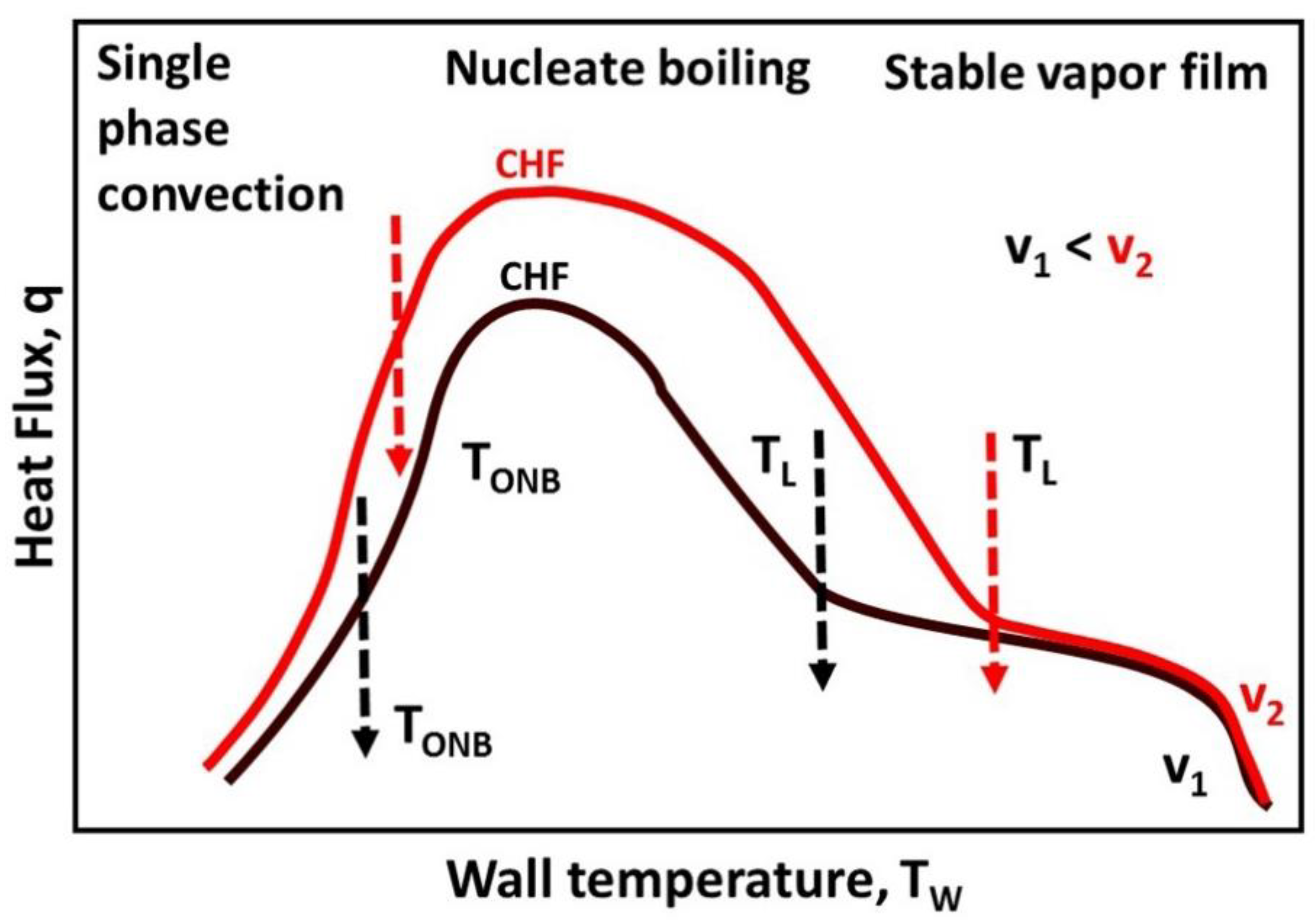
Liquid velocity refers to the relative velocity between the workpiece and the liquid. Since it is known that fluid velocity changes from point to point, then which velocity value is commonly considered to report the effect of liquid velocity on the boiling curve? The answer is not unique, but there are several conventional values. For example, for pool boiling quenching, a zero liquid velocity is reported in spite of the natural flow promoted by the buoyant force and the rising bubbles around the workpiece. Some authors report the liquid velocity during forced convection in agitated tanks by propeller driven flow, as the shaft rotation speed, in revolutions per minute (RPM). In other cases, forced convection is also obtained from a circulating flow through a quenching tank. A liquid flow rate enters the tank through an inlet tube and leaves the tank out through an outlet located somewhere far away. In this case, fluid velocity is taken as the average liquid velocity in a given cross section area, for example, at the inlet tube. Recently [31,32], it has been proposed to use the isothermal shear stress on the wall to correlate with boiling heat flux, inspired by the Reynolds–Colburn analogy, rather than using the liquid velocity itself. In spite there is no universal agreement on which liquid velocity to report, it is well known that increasing liquid velocity improves heat transfer from the workpiece as was shown by Totten and Lally from observations in a physical model of a quenching tank [33]. This fact has led to an important technological development called intensive quenching [34] where high pressure sprays are used to promote a very high cooling rate, leading to maximum surface compressive stresses, and avoiding workpiece surface cracking. Figure 4 shows schematically the effect of the liquid velocity on a boiling curve. Notice that fluid velocity has an effect on the CHF and on the transition temperatures, TL and TONB. This is associated to a higher fluid velocity in the boundary layer. At a high velocity, the contact time between liquid and solid is very short and therefore liquid cannot reach its boiling temperature. Then, single phase convection takes place improving the magnitude of heat flux. This regime can also improve uniformity on the heat flux as explained in Figure 3a,b. At a higher wall temperature, liquid flowing at velocity v2 is able to remove the vapor blanket as compared to liquid flowing slower. Therefore, Leidenfrost temperature increases with liquid velocity.
4.3. The Need for a Comprehensive Data Base for Heat Treatment Analysis
Ideally, thermophysical properties of alloys and quenchant liquids, mechanical properties of phases and microconstituents that are present in solid alloys, and a full data set of empirical parameters for phase transformation kinetic models would be enough to feed computerized models of heat transfer phenomena, phase transformation kinetics and mechanical behavior to predict the resulting microstructure and properties distribution in any workpiece subjected to a specific heat treatment. However, our current knowledge on convection boiling is not complete enough to predict, from first principles, the thermal evolution of actual workpieces during immersion quenching. An accurate prediction of nucleation, growth and detachment of multiple vapor bubbles from the wall surface requires to solve the multiphase fluid flow equations for turbulent flow conditions. Turbulent flow itself is a developing area that is currently best modeled by Direct Numerical Simulation (DNS). This method needs very fine grids and extremely small time steps to obtain accurate numerical solutions, demanding prohibitive computer effort for quenching simulation. Therefore, analysis of heat transfer during quenching is more conveniently carried out using alternative simplifying assumptions. These assumptions may be: (1) Isothermal fluid flow, (2) conjugate heat transfer, (3) interpenetrated liquid-vapor phases, or (4) using experimental thermal analysis and the solution of the IHCP.
The approach by isothermal fluid flow includes only the solution of the continuity and momentum equation in the liquid under steady and turbulent conditions [31,35]. The temperature evolution of the solid workpiece is not considered in this analysis. The fluid flow field is computed in the whole quenching tank that contains one or several workpieces under treatment. Velocity distribution is used to infer, qualitatively, the cooling rate of the workpiece [31] or use it to estimate a heat transfer coefficient from separate heat transfer calculations [35]. The higher the liquid velocity passing on the workpiece is, the higher the rate of heat removal would be. This approach is useful to study the effect that changes on the flow direction and magnitude have on the uniformity of heat removal from the workpiece.
The method based on conjugate heat transfer includes the calculation of both, fluid-dynamics of the quenchant and temperature evolution in the workpiece. No heat transfer coefficient is required in this approach since the heat flux at the wall surface is computed by specifying that both, heat flux and temperature are continuous at the wall surface, and thereby are computed. In this method, no boiling is considered since the liquid flows isothermally. This approach demands more computer effort than the purely isothermal flow model, however, it allows to compute cooling rates in the solid. These cooling rates are the basis to predict microstructure evolution and properties.
A more elaborate approach is the multiphase flow method represented by the interpenetrated liquid-vapor phases. The solid temperature can be computed or assumed equal to a fixed value, and the fluid flow calculations include boiling of liquid. In this approach, the rate of vaporization is computed but the interface of individual bubbles is not represented explicitly. Rather, volume fractions of vapor and liquid are determined for every control volume, that is for every position in the fluid. This is why the method takes the name interpenetrated phases. Bubble size should be specified but only to compute the rate of mass, momentum and energy interchange with the liquid, which is important to determine buoyant and drag forces and vaporization-condensation rates. In this regard, empirical coefficients for the rates of vaporization and condensation should be known. This approach requires more computer effort than the two previous methods but a greater detail in the quenching rate distribution over the wall surface can be obtained.
Finally, the most used method—both simple and trustworthy—is thermal analysis using the solution of the IHCP. As was mentioned above, a metallic probe is instrumented with one or several sub-superficial thermocouples. The instrumented probe is heated up to the homogenization temperature and then removed from the furnace and quenched. Each cooling curve is used in the solution of the Inverse Heat Conduction Problem to determine the heat flux at the wall as a function of time. The heat transfer coefficient can be computed from this heat flux using Equation (2). In essence, this procedure measures the temperature evolution at one, or more points, within the workpiece and then uses the solution of the IHCP to compute the temperature evolution in the rest of the workpiece. The main drawback of this approach is the need to generate thermal analysis for every needed quenching condition. For example, when using different quenchants, different alloys, different workpiece sizes, quenching under different liquid velocities, etc. Extrapolation of the obtained results for the studied cases is not recommended for other new cases.
There are standard instrumented probes [7] that are employed to characterize the quenching power of liquids. These probes are made of Inconel, stainless-steel or silver, which do not suffer a phase transformation in the solid-state during quenching. This is convenient to analyze the respective cooling curve data since no latent heat of phase transformation should be considered. An extension of this idea is to use instrumented probes made of the same steel grade under heat treatment [36]. These probes are processed in the quenching tank as if they were the quenching workpieces, emulating the actual production conditions.
4.4. Research Opportunities
The previous overview allows to identify the following research opportunities:
Mathematical modeling of heat transfer. Heat transfer coefficient is the key variable to simulate the thermal field evolution in a steel workpiece. However, overwhelmingly of technical papers considers that this coefficient is only a function of wall temperature, fluid velocity and its properties, and at best surface roughness. All these variables correspond to the region from the wall surface to the liquid. We do not agree with this idea. The resulting heat transfer coefficient also depends on the steel thermophysical properties and on the thermal gradients in the workpiece. This is because the net heat flux at the wall surface is the result of coupling heat conduction and convection boiling. There are few authors who report, implicitly, such an idea. For example, in ref. [2], heat transfer coefficient is also a function of position on the workpiece surface and time. The authors do not explain additional factors, other than fluid flow, affecting this dependence. We believe that such a dependence with position and/or time is not a proper choice because it hides the real physics behind it. For this reason, there is opportunity to develop mathematical models considering coupling between heat conduction in the steel and convection boiling in the fluid. The main physical ingredients controlling this coupling, remain to be investigated.
Experimental fluid flow and heat transfer. Laboratory measurements of heat flux are generally concentrated on the solid cooling curves. However, simultaneous fluid flow may be also characterized. There is a challenge of observing and recording the fluid flow field in very short periods, during cooling of the probe. An alternative strategy is to compute the actual convective boiling flow field rather than measure it. Therefore, analysis would include measured cooling curves in the solid and computed fluid flow field.
5. Conclusions
The analysis and criticism of the technical literature on heat transfer phenomena during solid steel quenching has led to the following conclusions.
- The low initial heat flux value in the boiling curve has been historically associated to the time constant of the thermocouple. Furthermore, at high wall temperatures, a stable vapor blanket may form acting as a thermal resistance to limit the heat flux. However, the measured heat flux in presence of this vapor blanket is larger than the initial heat flux. Therefore, the proposed argument based on the initial uniform temperature in the solid is a plausible explanation for such a low initial heat flux. Heat flux is promoted in the solid only after there is a thermal gradient in this material.
- It is known that heat flux removed from a quenching workpiece increases with fluid velocity. However, in spite of its importance, velocity has been reported as an average value and using different definitions. For example, rotation speed of a propel (RPM), average liquid velocity through the cross-section area of the inlet tube, or a local value which is proportional to the isothermal shear stress and pressure on the wall surface. This makes a comparison between results from different researchers difficult. In addition, a generalization of these results to integrate a data base becomes complex.
- Ideally, heat flux during quenching should be high and uniform above the workpiece surface. This would promote a uniform phase transformation throughout the whole workpiece minimizing thermal and phase formation stresses. According to the literature analysis carried out by the present authors, the best heat transfer regime to achieve such a uniformity is the single-phase convection, not the nucleation boiling regime, as it may be though because of the CHF. During single phase convection, liquid is always in contact with the wall surface minimizing heat flux fluctuations. Furthermore, the heat flux can be increased by augmenting the fluid velocity. For example, using a high-pressure spray. This increment in the liquid velocity would also increase the value of TONB, avoiding bubble formation on the wall.
- Mathematical modeling of the quenching process has been based on the solution of the conservation of mass, momentum and energy differential equations. Quenching modeling has been useful to understand the involved phenomena. However, there is no unique formulation to represent this complex process and a number of alternatives have been developed. From the literature analysis, we found models that can be classified into these categories: (1) Isothermal fluid flow, (2) conjugate heat transfer, (3) interpenetrated liquid-vapor phases, or (4) using experimental thermal analysis and the solution of the IHCP. The ultimate users should select the approach method, according to their particular objectives and their technical capabilities.
Author Contributions
Writing-original draft preparation, M.d.J.B.-R.; supervision, writing-review and editing, F.A.A.-G.; writing-review and editing, M.M.T.-R. All authors have read and agreed to the published version of the manuscript.
Funding
This research received no external funding.
Institutional Review Board Statement
Not applicable.
Informed Consent Statement
Not applicable.
Data Availability Statement
The used data can be found in the respective references.
Acknowledgments
The authors express gratitude to their respective Institutions for the support received during this pandemic, Covid-19.
Conflicts of Interest
The authors declare no conflict of interest.
References
- Totten, G.E.; Bates, C.E.; Clinton, N.A. Handbook of Quenchants and Quenching Technology; ASM International: Materials Park, OH, USA, 1993. [Google Scholar]
- Simsir, C. Modeling and Simulation of Steel Heat Treatment-Prediction of Microstructure, Distortion, Residual Stresses, and Cracking. In ASM Handbook Steel Heat Treating Technologies; Dosset, J., Totten, G.E., Eds.; ASM International: Materials Park, OH, USA, 2014; Volume 4B. [Google Scholar]
- Abbasi, B.; Kim, J.; Marshal, A. Dynamic pressure based prediction of spray cooling heat transfer coefficients. Int. J. Multiph. Flow 2010, 36, 491–502. [Google Scholar] [CrossRef]
- Araki, K.; Yoshinobu, S.; Nakatani, Y.; Moriyama, A. Stationary measurement for heat transfer coefficient in droplet-cooling of hot metal. Trans. ISIJ 1982, 22, 952–958. [Google Scholar] [CrossRef] [Green Version]
- Bernardin, J.D.; Mudawar, I. Film boiling heat transfer of droplet steams and sprays. Int. J. Heat Mass Transf. 1997, 40, 2579–2593. [Google Scholar] [CrossRef]
- Hernández-Bocanegra, C.A.; Castillejos-Escobar, A.H.; Acosta-González, F.A.; Zhou, X.; Thomas, B.G. Measurement of heat flux in dense air-mist cooling: Part I—A novel steady-state technique. Exp. Therm. Fluid Sci. 2013, 44, 147–160. [Google Scholar] [CrossRef]
- Kobasko, N.I. Thermal Equilibrium and Universal Correlation for Its Heating-Cooling Time Evaluation. Theor. Phys. Lett. 2021, 29, 205–219. [Google Scholar] [CrossRef]
- Stewart, I.; Massingham, J.D.; Hagers, J.J. Heat transfer coefficient effects on spray cooling. Iron Steel Eng. 1996, 73, 17–23. [Google Scholar]
- Li, D.; Wells, M.A.; Cockcroft, S.L.; Caron, E. Effect of Sample Start Temperature during Transient Boiling Water Heat Transfer. Metall. Mater. Trans. B 2007, 38, 901–910. [Google Scholar] [CrossRef]
- Beck, J.V. Nonlinear estimation applied to the nonlinear inverse heat conduction problem. Int. J. Heat Mass Transf. 1970, 13, 703–716. [Google Scholar] [CrossRef]
- Babu, K.; Kumar, T.S.P. Mathematical Modeling of Surface Heat Flux During Quenching. Metall. Mater. Trans. B 2010, 41, 214–224. [Google Scholar] [CrossRef]
- Rabin, Y.; Rittel, D. A Model for the Time Response of Solid-embedded Thermocouples. Exp. Mech. 1999, 39, 132–136. [Google Scholar] [CrossRef]
- Incropera, P.I.; Dewitt, D.P. Fundamentals of Heat and Mass Transfer, 3rd ed.; John Wiley and Sons: New York, NY, USA, 1990; p. 393. ISBN 0-471-61246-4. [Google Scholar]
- Passarella, D.N.; Aparicio, A.; Varas, F.; Ortega, E.B. Heat Transfer Coefficient Determination of Quenching Process. In Mecánica Computacional, Proceedings of the Asociación Argentina de Mecánica Computacional, San Carlos de Bariloche, Argentina, 23–26 September 2014; Bertolino, G., Cantero, M., Storti, M., Teruel, Y.F., Eds.; Asociación Argentina de Mecánica Computacional: Santa Fe, Argentina, 2014; Volume XXXVIII, pp. 2009–2021. [Google Scholar]
- Fernandes, P.; Prabhu, K.N. Effect of section size and agitation on heat transfer during quenching of AISI 1040 steel. J. Mater. Process Technol. 2007, 183, 1–5. [Google Scholar] [CrossRef]
- Aronsson Rinby, C.; Sahlin, A. Compilation and Validation of Heat Transfer Coefficients of Quenching Oils. Master’s Thesis, Chalmers University of Technology, Gothenburg, Sweden, 2012. [Google Scholar]
- Shahriari, A.; Hermes, M.; Bahadur, V. Electrical control and enhancement of boiling heat transfer during quenching. Appl. Phys. Lett. 2018, 108, 091607. [Google Scholar] [CrossRef]
- Muhieddine, M.; Canot, E.; March, R. Various Approaches for Solving Problems in Heat Conduction with Phase Change. Int. J. Finite Vol. 2009, 6, 1–19. [Google Scholar]
- Camporredondo, S.J.E.; Castillejos, E.A.H.; Acosta, G.F.A.; Gutiérrez, M.E.P.; Herrera, G.M.A. Analysis of Thin-Slab Casting by the Compact-Strip Process: Part I. Heat Extraction and Solidification. Metall. Mater. Trans. B 2004, 35, 541–560. [Google Scholar] [CrossRef]
- Durand, D.; Durban, C.; Girot, F. Coupled Phenomena and Modeling of Material Properties in Quench Hardening Following Inductive Heating of the Surface. In Proceedings of the 17th ASM Heat Treating Society Conference including the 1st International Induction Heat Treating Symposium, Indianapolis, IN, USA, 15–18 September 1997; Milam, D., Poteet, D.A., Pfaffman, G.D., Rudnev, V., Muehlbauer, A., Albert, W.B., Eds.; ASM International: Materials Park, OH, USA, 1997; pp. 855–863. [Google Scholar] [CrossRef]
- Lopez-Garcia, R.D.; Garcia-Pastor, F.A.; Castro-Roman, M.J.; Alfaro-Lopez, E.; Acosta-Gonzalez, F.A. Effect of Immersion Routes on the Quenching Distortion of a Long Steel Component Using a Finite Element Model. Trans. Indian Inst. Met. 2016, 69, 1645–1656. [Google Scholar] [CrossRef]
- Sánchez-Sarmiento, G.; Castro, M.; Totten, G.E.; Harvis, L.; Webster, G.; Cabré, M.F. Modeling Residual Stresses in Spring Steel Quenching. In Proceedings of the 21st ASM Heat Treating Society Conference, Indianapolis, IN, USA, 5–8 November 2001; Liščić, B., Tensi, H.M., Shrivastava, S., Specht, F., Eds.; ASM International: Materials Park, OH, USA, 2001; pp. 1–10. [Google Scholar]
- Poirier, D.R.; Geiger, G.H. Correlations and Data for Heat Transfer Coefficients. In Transport Phenomena in Materials Processing, 2nd ed.; The Minerals Metals & Materials Society: Warrendale, PA, USA; Springer International Publishing: Cham, Switzerland, 2016. [Google Scholar] [CrossRef]
- Standard Test Methods for Determining Hardenability of Steel; ASTM International: West Conshohocken, PA, USA, 2007; pp. 18–26.
- Smoljan, B.; Iljkić, D.; Totten, G.E. Mathematical Modeling and Simulation of Hardness of Quenched and Tempered Steel. Metall. Mater. Trans. B 2015, 46, 2666–2673. [Google Scholar] [CrossRef]
- Motomochi-Espinoza, P.A.; Acosta-González, F.A. A Method to Design Laboratory Tests Aimed to Determine the Heat Flux during Steel Processing (in Spanish). In Proceedings of the Memorias del 37° Congreso Internacional de Metalurgia y Materiales, Saltillo, Coahuila, Mexico, 11–13 November 2015; Tecnológico Nacional de México: Mexico City, Mexico, 2015; pp. 223–9540. [Google Scholar]
- Arimoto, K.; Li, G.; Arvind, A.; Wu, W.T. The Modeling of Heat Treating Process. In Proceedings of the 18th Conference of Heat Treating, 12–15 October 1998; Wallis, R.A., Walton, H.W., Eds.; ASM International: Materials Park, OH, USA, 1998; pp. 23–30. [Google Scholar] [CrossRef]
- Rohde, J.; Thuvander, A.; Melander, A. Using thermodynamic information in numerical simulation of distortion due to heat treatment. In Proceedings of the 5th ASM Heat Treatment and Surface Engineering Conference in Europe Incorporating the 3rd International Conference on Heat Treatment with Atmospheres, Gothenburg, Sweden, 7–9 June 2000; Mittemeijer, E.J., Grosch, J., Eds.; ASM International: Materials Park, OH, USA, 2000; pp. 21–29. [Google Scholar] [CrossRef]
- Esfahani, A.K.; Babaei, M.; Sarrami-Foroushani, S. A numerical model coupling phase transformation to predict microstructure evolution and residual stress during quenching of 1045 steel. Math. Comput. Simul. 2021, 179, 1–22. [Google Scholar] [CrossRef]
- Agarwal, P.K.; Brimacombe, J.K. Mathematical Model of Heat Flow and Austenite-Pearlite Transformation in Eutectoid Carbon Steel Rods for Wire. Metall. Mater. Trans. B 1981, 12, 121–133. [Google Scholar] [CrossRef]
- Barrena-Rodríguez, M.J.; González-Melo, M.A.; Acosta-González, F.A.; Alfaro-López, E.; García-Pastor, F.A. An Efficient Fluid-Dynamic Analysis to Improve Industrial Quenching Systems. Metals 2017, 7, 190. [Google Scholar] [CrossRef] [Green Version]
- González-Melo, M.A.; Acosta-González, F.A. Efficient Prediction of Heat Transfer during Quenching based on a Modified Reynolds-Colburn Analogy. In Proceedings of the Thermal Processing in Motion including the 4th International Conference on Heat Treatment and Surface Engineering in Automotive Applications, Spartanburg, SC, USA, 5–7 June 2018; Ferguson, L., Frame, L., Goldstein, R., Guisbert, D., Scott MacKenzie, D., Eds.; ASM International: Materials Park, OH, USA, 2018; pp. 91–97. [Google Scholar]
- Totten, G.E.; Lally, K.S. Proper Agitation Dictates Quench Success Part 1. Heat Treat. 1992, 9, 12–17. [Google Scholar]
- Aronov, M.A.; Kobasko, N.I.; Powell, J.A.; Young, J. Practical application of intensive quenching technology for steel parts and real time quench tank mapping. In Proceedings of the 19th ASM Heat Treating Society Conference, Cincinnati, OH, USA, 1–4 November 1999; Krauss, G., Midea, S.J., Pfaffmann, G.D., Eds.; ASM International: Materials Park, OH, USA, 1999; pp. 1–9. [Google Scholar]
- MacKenzie, S.; Li, Z.; Ferguson, B.L. Effect of Quenchant Flow on the Distortion of Carburized Automotive Pinion Gears. In Proceedings of the 5th International Conference on Quenching and Control Distortion including European Conference on Heat Treatment 2007, Berlin, Germany, 25–27 April 2007; International Federation for Heat Treatment and Surface Engineering: Winterthur, Switzerland, 2007; pp. 1–11. [Google Scholar]
- Kumar, T.S.P. Influence of Steel Grade on Surface Cooling Rates and Heat Flux during Quenching. J. Mater. Eng. Perform. 2013, 22, 1848–1854. [Google Scholar] [CrossRef]
Figure 1.
Graphic summary of the boiling curve determination from a cooling curve and using the solution of the IHCP. The workpiece is an instrumented steel cylinder for the end-quenched Jominy test.
Figure 1.
Graphic summary of the boiling curve determination from a cooling curve and using the solution of the IHCP. The workpiece is an instrumented steel cylinder for the end-quenched Jominy test.

Figure 2.
Schematic representation of (a) boiling curves corresponding to the continuous cooling of probes from several initial temperatures, T1, T2, …, T6 and (b) heat transfer regimes during quenching by immersion.
Figure 2.
Schematic representation of (a) boiling curves corresponding to the continuous cooling of probes from several initial temperatures, T1, T2, …, T6 and (b) heat transfer regimes during quenching by immersion.

Figure 3.
Schematic comparison of heat transfer distribution from a workpiece when quenching under: (a) nucleation boiling regime, in which heat flux through vapor bubbles is smaller than heat flux to the liquid and (b) single phase convection regime, where heat flux in uniform through the wall surface.

Figure 4.
Schematic representation on the effect of liquid velocity on the boiling curve. Notice that Leidenfrost (TL) and onset of nucleate boiling (TONB) temperatures change with fluid velocity, where velocity v1 is smaller than velocity v2.
Figure 4.
Schematic representation on the effect of liquid velocity on the boiling curve. Notice that Leidenfrost (TL) and onset of nucleate boiling (TONB) temperatures change with fluid velocity, where velocity v1 is smaller than velocity v2.


Table 1.
Experimentally determined heat transfer coefficients as a function of fluid velocity.
| Reference | Fluid Velocity 1 | |||
|---|---|---|---|---|
| Comments | Heat Transfer Coefficient (W/m2K) | |||
| Ref. [14] 2 | 0 rpm 4246 | 1000 rpm 4459 | 2000 rpm 4671 | 3000 rpm 4883 |
| Oil Q8 Bellini FNT® at 66 °C | ||||
| Probe initial temperatures: 750, 800, 850 and 900 °C | ||||
| Ref. [15] 2,3 | 0 m/s, 28 mm 2697 | 0 m/s, 44 mm 3848 | 0.33 m/s, 28 mm 4348 | 0.33 m/s, 44 mm 5635 |
| Mineral oil at 30 °C Probe initial temperature: 870 °C | ||||
| Ref. [16] | 0 m/s 3000 | 0.2 m/s 3100 | 0.35 m/s 3500 | 0.5 m/s 3900 |
| Oil Quenchway 125B at 130 °C | ||||
| Probe initial temperature 850 °C | ||||
1 Units may be rpm or m/s as it is indicated. 2 Computed values from CHF, Tmax and Tf data. 3 28 and 44 mm are the diameters of cylindrical probes, steel grade AISI 1040.
Publisher’s Note: MDPI stays neutral with regard to jurisdictional claims in published maps and institutional affiliations. |
© 2021 by the authors. Licensee MDPI, Basel, Switzerland. This article is an open access article distributed under the terms and conditions of the Creative Commons Attribution (CC BY) license (https://creativecommons.org/licenses/by/4.0/).
Share and Cite
MDPI and ACS Style
Barrena-Rodríguez, M.d.J.; Acosta-González, F.A.; Téllez-Rosas, M.M. A Review of the Boiling Curve with Reference to Steel Quenching. Metals 2021, 11, 974. https://0-doi-org.brum.beds.ac.uk/10.3390/met11060974
AMA Style
Barrena-Rodríguez MdJ, Acosta-González FA, Téllez-Rosas MM. A Review of the Boiling Curve with Reference to Steel Quenching. Metals. 2021; 11(6):974. https://0-doi-org.brum.beds.ac.uk/10.3390/met11060974
Chicago/Turabian StyleBarrena-Rodríguez, Manuel de J., Francisco A. Acosta-González, and María M. Téllez-Rosas. 2021. "A Review of the Boiling Curve with Reference to Steel Quenching" Metals 11, no. 6: 974. https://0-doi-org.brum.beds.ac.uk/10.3390/met11060974
Note that from the first issue of 2016, this journal uses article numbers instead of page numbers. See further details here.