Numerical Study of Epitaxial Growth after Partial Remelting during Selective Electron Beam Melting in the Context of Ni–Al

Abstract

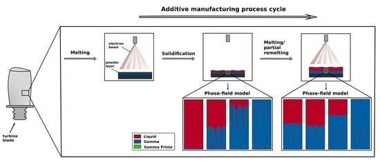
In the selective electron beam melting approach an electron beam is used to partially melt the material powder. Based on the local high energy input, the solidification conditions and likewise the microstructures strongly deviate from conventional investment casting processes. The repeated energy input into the material during processing leads to the partial remelting of the already existing microstructure. To closer investigative this effect of partial remelting, in the present work the phase-field model is applied. In the first part the solidification of the referenced Ni–Al system is simulated in respect to selective electron beam melting. The model is calibrated such to reproduce the solidification kinetics of the superalloy CMSX-4. By comparison to experimental observations reported in the literature, the model is validated and is subsequently applied to study the effect of partial remelting. In the numerical approach the microstructures obtained from the solidification simulations are taken as starting condition. By systematically varying the temperature of the liquid built layer, the effect of remelting on the existing microstructure can be investigated. Based on these results, the experimental processing can be optimized further to produce parts with significantly more homogenous element distributions.

1. Introduction

Based on the outstanding material properties and the high degree of freedom in design, the production technology of additive manufacturing (AM) becomes increasingly relevant in the research field of material science. The term AM compiles various different techniques, in [1] a good overview is given. One technique, which is frequently applied, is selective electron beam melting (SEBM). During processing an electron beam is used to melt the volume of the metal powder which represents the contour of the later cast part. In [2] a good summary of the SEBM methodology and the technical developments is presented. One advantage of the SEBM process is the possibility to produce single crystalline (SX) microstructures as reported in [3,4]. The high local energy input results in remarkable solidification conditions, more precisely high thermal gradients and cooling rates. These solidification conditions significantly differ from conventional investment casting. As consequence, the microstructure of the materials processed by SEBM strongly deviates from conventionally casted SX materials. Based on the high solidification velocities, the solute redistribution is constrained leading to less pronoun segregation profiles as presented in [5,6]. That leads to improved material properties compared to parts produced by conventional investment casting as shown in [7]. To enhance the understanding of the underlying physical phenomena, various models can be applied to simulate microstructure evolution during processing [8,9,10]. In [11], the most widely used modelling approaches are presented in detail. One of those approaches is the phase-field method, which is particularly suitable to study the microstructural evolution (e.g., [12,13,14]). In the work of Warnken et al. the phase-field method is used to study the microstructure evolution within CMSX-4 samples in context of the investment casting process and the subsequent heat treatment [15]. One characteristic of the AM technology is the layer-by-layer approach, which leads to a repeated heat input into the processed material. This energy input has a strong influence on the already solidified layers, respectively, the corresponding microstructures. In the work of Schwerdtfeger et al., in context of the SEBM process of the Ti–Al–Nb–Cr system, evidence is reported, that the cyclic heating up of the system leads to solid–solid phase transformations which are not observed after solidification [16]. In their work [17], Koepf et al. show numerical results for the grain evolution within a CMSX-4 sample produced by SEBM whereby the effect of remelting is considered in the simulations. Certainly in the literature no study referring to the microscale can be found, which addresses the influence of the effect of partial remelting on the existing dendritic microstructure.

2. Materials and Methods

2.1. Model Description

To model the microstructural evolution during solidification, the phase-field model has become very popular in recent decades (e.g., [15,18,19,20,21]). To account for the heterogeneous microstructure of the referenced alloy, the multi phase-field approach as postulated by Steinbach et al. is applied [18]. In detail, the referenced system consists of the liquid phase, the austenitic $\gamma$-phase and the intermetallic $\gamma$’-phase. The evolution equation for the phase-field (of phase $\alpha$) is expressed in Equation (1).

$$\dot{{\varphi }_{\alpha }}=-\sum _{\beta }^N\frac{{\pi }^2{M}_{\alpha \beta }}{8\eta N}\left[\frac{\delta F}{\delta {\varphi }_{\alpha }}-\frac{\delta F}{\delta {\varphi }_{\beta }}\right]$$

(1)

In Equation (1) $M_{\alpha \beta }$ represents the interface mobility, F is the energy functional, $\eta$ is the interface width and N is the number of phases. Equation (1) references the phase change between two phases or grains ($\alpha$ and $\beta$), whereby the model can be extended to multiple phases or grains, details can be found in [18,22]. In context of Equation (1), the sum constraint:

$$\sum _{\alpha =1\dots N}{\varphi }_{\alpha }=1$$

is valid at every point within the simulation domain. The energy functional F in Equation (1) comprises of multiple contributions, e.g., the interface free energy, the chemical free energy and the elastic free energy as can be concluded from Equation (2).

$$F=f_{\mathrm{chem}.}+f_{\mathrm{int}.}+f_{\mathrm{elas}.}$$

(2)

In the present work the elastic contribution from Equation (2) is neglected, the description of the chemical and the interface free energy is presented in Equations (3) and (4).

$$f_{\mathrm{chem}.}=\sum _{\alpha =1}^N{\varphi }_{\alpha }{f}_{\alpha }\left(c_{\alpha }\right)+\lambda \left[c-\sum _{\alpha =1}^N\left({\varphi }_{\alpha }{c}_{\alpha }\right)\right]$$

(3)

$$f_{\mathrm{int}.}=\sum _{\alpha \ne \beta }\frac{4{\sigma }_{\alpha \beta }}{\eta }\left[-\frac{{\eta }^2}{{\pi }^2}\nabla {\varphi }_{\alpha }·\nabla {\varphi }_{\beta }+{\varphi }_{\alpha }{\varphi }_{\beta }\right]$$

(4)

In Equation (3) $f_{\alpha }\left(c_{\alpha }\right)$ represents the bulk free energies of the considered phases whereby c${}_{\alpha }$ comprises all concentrations of the phase $\alpha$ in the form of a vector. Analogous c represents the concentrations of all referenced phases and $\lambda$ is the chemical potential. In Equation (4) ${\sigma }_{\alpha \beta }$ is the interface energy of the phases $\alpha$ and $\beta$. Inserting F in Equation (1) and applying further mathematical operations leads to the evolution equation of the phase-field as presented in Equation (5), details can be found in [23].

$$\dot{{\varphi }_{\alpha }}=\sum _{\beta =1\dots n}{M}_{\alpha \beta }\left\{{\sigma }_{\alpha \beta }\left[{\varphi }_{\beta }{\nabla }^2{\varphi }_{\alpha }-{\varphi }_{\alpha }{\nabla }^2{\varphi }_{\beta }+\frac{{\pi }^2}{2{\eta }^2}\left({\varphi }_{\alpha }-{\varphi }_{\beta }\right)\right]+\frac{\pi }{\eta }\sqrt{{\varphi }_{\alpha }{\varphi }_{\beta }}\Delta g_{\alpha \beta }\right\}$$

(5)

In Equation (5) ${\eta }_{\alpha \beta }$ is the interface width and $\Delta$$g_{\alpha \beta }$ is the driving force contribution. In general ${\varphi }_{\alpha }$ represents an indicator function, the values of ${\varphi }_{\alpha }$ vary in the range from 0 to 1, whereby 0 represents the liquid state and 1 the solid state. Based on that approach, the evolution of the interface of the considered phase(s), in Equation (5) it is phase $\alpha$, can be tracked and described. To model the dendritic growth during solidification, besides the phase field the temperature and the concentration fields need to be considered to account for thermosolutal interactions. With respect to Equation (5), the contributions of the concentration and the temperature field are included by the (thermodynamic) driving force term $\Delta$$g_{\alpha \beta }$. The evolution of the concentration field of phase $\alpha$ can be expressed by Equation (6).

$$\dot{c}=\nabla \left\{{\varphi }_{\alpha }\sum _{\alpha }\left[D^{\alpha }\nabla c_{\alpha }\right]+\sum _{\alpha \beta }{J}_{\alpha \beta }\right\}$$

(6)

In Equation (6) D represents the diffusion coefficient and $J_{\alpha \beta }$ is the anti-trapping current. In the phase-field model the interface is treated as diffuse interface, thereby $\varphi$ can vary in the range from 0 to 1. The anti-trapping current counteracts the solute trapping effect inherited by this diffuse interface approach. In the present work an anti-trapping current as presented in the work of Karma et al. is used, detailed information can be found in the literature [24,25,26]. To approximate the solution of the set of differential equations resulting from the multi phase-field formulation, the software suite OpenPhase is applied [27]. In [28], detailed information can be found regarding the mathematical implementation of the multi phase-field method in OpenPhase. To account for the correct thermal field evolution during the solidification, respectively, the remelting of the system, the phase field is additionally coupled to the temperature field as can be concluded from Equation (7). Equation (7) describes the evolution of the temperature field.

$$\dot{T}=\nabla \left(\lambda \nabla T\right)+\frac{{\mathrm{L}}_{\mathrm{i}=1..\mathrm{n}\left(\mathrm{solid}\right)}}{c_p}\sum _{\mathrm{i}=1\dots \mathrm{n}\left(\mathrm{solid}\right)}{\dot{\varphi }}_i$$

(7)

In Equation (7) $\lambda$ represents the thermal conductivity, T is the temperature, L${}_{\mathrm{i}}$ is the latent heat of all considered solid phases, $c_p$ is the heat capacity and ${\varphi }_i$ is the phase field. To approximate the solution of Equation (7), an implicit algorithm based on the Gauss–Seidel approach is used (details can be found in the Appendix A). In the applied algorithm the stencil is defined with a width of one grid point in each direction (x, y, z). The simulation results are benchmarked to the analytical solution (in 1D) of the heat kernel which is presented in Equation (8).

$$\Phi \left(x,t\right)=\frac{1}{{\sqrt{4\pi \lambda t}}^1}ex{p}^{\left(-\frac{|x^2|}{4\lambda t}\right)}$$

(8)

The simulation results as well as the results from the analytical solution are compiled in

Table 1. Results for the temperature of the reference point obtained by the analytical solution and the corresponding error (Err.) of the simulation results for different time steps and time step increments ($\Delta t$).

t [s]	${\mathbf{T}}_{\mathbf{analytical}}\left[\mathbf{K}\right]$	$\mathbf{Err}{.}_{\mathbf{\Delta }\mathbf{t}=0.01}\left[\mathbf{K}\right]$	$\mathbf{Err}{.}_{\mathbf{\Delta }\mathbf{t}=0.1}\left[\mathbf{K}\right]$	$\mathbf{Err}{.}_{\mathbf{\Delta }\mathbf{t}=1}\left[\mathbf{K}\right]$	$\mathbf{Err}{.}_{\mathbf{\Delta }\mathbf{t}=10}\left[\mathbf{K}\right]$
10	1.3031$·$10${}^{-9}$	3.416$·$10${}^{-9}$	6.6931$·$10${}^{-9}$	1.2531$·$10${}^{-7}$	1.0997$·$10${}^{-5}$
100	1.6680$·$10${}^{-4}$	1.0905$·$10${}^{-7}$	1.5984$·$10${}^{-7}$	6.5558$·$10${}^{-7}$	4.6046$·$10${}^{-6}$
1000	6.8066$·$10${}^{-5}$	1.8086$·$10${}^{-6}$	1.809$·$10${}^{-6}$	1.8128$·$10${}^{-6}$	1.8525$·$10${}^{-6}$
10,000	7.8344$·$10${}^{-6}$	6.6543$·$10${}^{-6}$	6.6543$·$10${}^{-6}$	6.6541$·$10${}^{-6}$	6.6528$·$10${}^{-6}$

.

The values presented in Table 1 refer to a predefined reference point with the known distance x to the heat source. For simplicity all other input parameters are set to 1. The simulation results indicate an acceptable deviation from the analytical solution of 6.6$·$10${}^{-6}$ K for different time increments which vary by a factor of 1000 as can be concluded from Table 1. Based on the implicit formulation, larger time increments can be chosen for the simulation. The heat diffusion references significantly smaller time scales compared to the solute diffusion, hence an explicit approximation approach would increase the required computational resources remarkably. In order to calculate the correct amount of released latent heat, the change of the fraction of the solid phase(s) is tracked at all cells with a defined distance to the interface. Proportional to the local change of the fraction of the solid phase(s), the latent heat is released at the interface. The total amount of the released latent heat is obtained by using the Scheil model which is implemented in the ThermoCalc software package (database TTNI7) [29].

2.2. Applied Input Data

In the present work the binary Ni–Al system is referenced with the nominal composition of 21 mole-% Al. The liquid phase, the $\gamma$-phase and the primary $\gamma$’-phase are considered. To guarantee a proper thermodynamic description of the system, the phase diagram is linearized in the region of interest as can be concluded from Figure 1, the corresponding slopes can be found in

Table 2. Relevant input parameters applied in the solidification simulations.

Parameter	Value
m${}_{01}$ (slope from Figure 1)	−8.0136 K/mole-% Al
m${}_{10}$	−8.8347 K/mole-% Al
m${}_{02}$	2.9846 K/mole-% Al
m${}_{20}$	6.9373 K/mole-% Al
m${}_{12}$	77.7003 K/mole-% Al
m${}_{21}$	188.5815 K/mole-% Al
Domain size (x, y, z)	(200$·$1$·$625) cells
Grid spacing	8.0$·$10${}^{-8}$ m
Time increment	1.0$·$10${}^{-8}$ s
Molar Volume Liquid	7.64$·$10${}^{-6}$ $\frac{{\mathrm{m}}^3}{\mathrm{mol}}$
Molar Volume $\gamma$	7.27$·$10${}^{-6}$ $\frac{{\mathrm{m}}^3}{\mathrm{mol}}$
Molar Volume $\gamma$’	7.0$·$10${}^{-6}$ $\frac{{\mathrm{m}}^3}{\mathrm{mol}}$
Interface energy liquid-$\gamma$, liquid-$\gamma$’	0.26 J$·$m${}^{-2}$
Start temperature	1663.0 K
Cooling rate	−10,000 K$·$s${}^{-1}$
Latent heat Liq.→ $\gamma$	139,252.71 J$·$Kg${}^{-1}$
Latent heat Liq.$\to \gamma$’	98,396.52 J$·$Kg${}^{-1}$
Thermal conductivity liquid	50.0 W$·$mK${}^{-1}$
Thermal conductivity $\gamma$, $\gamma$’	75.0 W$·$mK${}^{-1}$
Heat capacity liquid	810.75 J$·$K${}^{-1}$
Heat capacity $\gamma$, $\gamma$’	697.21 J$·$K${}^{-1}$
Interface mobility $\gamma$	7.5$·$10${}^{-8}$ m${}^4$$·$Js${}^{-1}$
Interface mobility $\gamma$’	9.0$·$10${}^{-8}$ m${}^4$$·$Js${}^{-1}$
Entropy of fusion $\gamma$	−0.8124$·$10${}^6$ J$·$m${}^{-3}$$·$K${}^{-1}$
Entropy of fusion $\gamma$’	−1.2188$·$10${}^6$ J$·$m${}^{-3}$$·$K${}^{-1}$

. The phase diagram in Figure 1 is obtained from ThermoCalc calculations.

In the simulations the $\gamma$’-phase is defined as stoichiometric phase with a fixed composition of 24.7 mole-% Al. To account for the correct solidification kinetics, the temperature dependence of the diffusion coefficient is considered by the use of the Arrhenius formulation. The diffusion coefficients resulting from the Arrhenius formulation for the diffusion of Al in the liquid and the solid phases coincide with data provided by Ni-base mobility databases as can be concluded from Figure 2. In Figure 2, the dashed lines refer to the Arrhenius formulation, the solid lines represent the data from the mobility database.

The dimensions of the simulation domain, which are presented in Table 2 amongst other relevant input parameters, correspond to the dimensions of one powder layer in the referenced experimental setup. Further information about the experimental processing can be found in [3].

The height of the simulation domain is 50 $\mathsf{\mu }$m whereas the width of the domain represents a section of the overall built layer with a thickness of 15 $\mathsf{\mu }$m motivated by the reduction of the required computation time. Based on that the sideways boundary conditions (BC) are defined as periodic for the phase field and the concentration field. This means the value of the (left) boundary is equal to the outermost value of the opposite boundary of the domain (on the right side). Thereby the dendrite growth outside the simulation domain can be considered to some extent. For the phase field and the concentration field the top and bottom BC is chosen such that the boundary value is equal to the outermost value of the corresponding field. In this way the gradient is zero and any flux out of the simulation domain is prevented. With respect to the temperature field, all boundaries are defined as no-flux BC besides the bottom BC. This BC is implemented as fixed value since it represents the cooling of the system at the bottom. In accordance with experimental values reported in [1] for the SEBM process, the cooling rate is set to −10,000 K$·$s${}^{-1}$. Thus, the cells of the bottom boundary are continuously cooled down by the defined cooling rate during the entire simulation time. The simulation domain is set up in 2D since the consideration of the fine primary $\gamma$’-particles requires a numerical resolution of at least 0.8 $\mathsf{\mu }$m. When applying such small grid spacing for the 3D simulation domain, the computational expanse increases drastically. To compensate the drawbacks of the 2D-domain approach, the model is calibrated such that the results of the simulations (in 2D) reproduce the correct solidification kinetics as observed in experimental analysis. This will be discussed in detail at a later stage. For the nucleation of the $\gamma$- respectively the $\gamma$’-phase, the free growth model based on the work of Greer et al. [30] is applied. The particle distribution is defined randomly, whereas the nucleation density is set to 5$·$10${}^{-22}$ m${}^{-3}$ ($\gamma$-phase), respectively, 5$·$10${}^{-25}$ m${}^{-3}$ ($\gamma$’-phase). The size distribution of the particles is defined by a normal distribution function which is presented in Equation (9), details can be found in [31].

$$N\left(d\right)=K·\frac{1}{b\sqrt{2\pi }}·exp\left[-\frac{{(d-a)}^2}{2b^2}\right]$$

(9)

In Equation (9) K represents the particle density, d is the diameter of the seed particle, a is the mean value and b is the standard deviation of the normal distribution function. By the use of the parameters a and b, the part of the distribution function can be specified, which should be used in the nucleation model. If the local system temperature is lower than the equilibrium liquidus temperature, more precisely by the amount of the required critical undercooling, the nuclei becomes stable and starts to grow. In that regard the critical undercooling is a combination of the thermal and the curvature undercooling. The curvature undercooling strongly depends on the diameter of the seed particle, hence the nuclei (within the range of the size distribution) with a lower critical undercooling will form at earlier time steps during the nucleation stage. When the nucleus becomes thermodynamically unstable during the further growth, e.g., due to the release of latent heat, the nucleus will dissolve. The orientation of the nuclei is set randomly in the range from 0° to 180°.

3. Results and Discussion

3.1. Microstructure Formation during Solidification

As can be seen from Figure 3, the nuclei of the $\gamma$-phase form at the bottom of the simulation domain as a result from the cooling boundary condition. Although the orientations of the nuclei are unrestricted, the particles orientated in the direction of the thermal gradient, more precisely in Z-direction, become stable. During the further growth, the more misorientated nuclei are overgrown and four stable dendrites evolve as can be concluded from Figure 3.

The primary dendrite arm spacing obtained from the simulation results is approximately 4 $\mathsf{\mu }$m which matches with experimental values reported by Ramsperger et al. [3,32]. As consequence of the high thermal gradients, the dendrites exhibit a cellular morphology as can be seen in Figure 3. This shape corresponds to experimental microstructure analysis carried out by Karimi et al. [33] in context of the SEBM process. The thermal gradient observed at the interface in the simulation results varies in the range from 125 to 185 $\mathrm{K} {\mathrm{mm}}^{-1}$. This is in good agreement with the value obtained by experiments which is 200 $\mathrm{K} {\mathrm{mm}}^{-1}$ as presented in [3]. As consequence of the small primary dendrite arm spacing, the dendrites form no secondary arms. In Figure 4, the release of the latent heat as well as the averaged system temperature is plotted over the simulation time.

In Figure 4, the released latent heat corresponds to the total amount of released latent heat per time step, the averaged system temperature is the mean value of all temperature values within the simulation domain. From the plot of the averaged system temperature the total time of solidification can be concluded, the inflection point at 3.2$·$10${}^{-4}$ s represents the end of solidification. Considering the height of the simulation domain of 50 $\mathsf{\mu }$m, the corresponding solidification velocity exhibits 16 mm$·$s${}^{-1}$ which is close to the experimentally determined value of 20 mm$·$s${}^{-1}$ [3]. Based on that coincidence it can be assumed, that the model reproduces the solidification kinetics correctly. At that point it needs to be mentioned, that the referenced experimental results address the complete alloy range of the superalloy CMSX-4. By the calibration of the model parameters, the solidification kinetics of the binary Ni–Al system can be adapted to the experimentally observed solidification kinetics of the CMSX-4 alloy. With regard to the magnification in Figure 4 it can be seen that the model is capable of reproducing the effect of recalescence at the beginning of solidification. Due to the solute redistribution during the further growth of the $\gamma$-phase, the interdendritic regions become highly enriched with Al as can be concluded from the Al concentration maps in Figure 3. When the local temperature comes below the liquidus temperature of the primary $\gamma$’-phase, the nucleation of $\gamma$’ is initiated. In case these nuclei become stable, the $\gamma$’-particles grow further in the volume of the interdendritic regions as can be seen from the magnification in Figure 3. The kinks in the plot of the released latent heat in Figure 4 correspond to the nucleation and the growth of the primary $\gamma$’-phase.

3.2. Microstructure Evolution during Remelting

For the analysis of the effect of partial remelting during the SEBM process, the results from the solidification simulations are taken as starting point. In this view the microstructure obtained from the solidification simulation represents the previous built layer. To reduce the required computational resources, one half of the solidification simulation results is used as can be concluded from Figure 5.

With respect to Figure 5, the upper half of the simulation domain represents the actual built layer. Therefore this volume of the domain is defined as liquid phase exhibiting the nominal alloy composition. The temperature of the liquid is set to 1900 K with regard to numerical analysis carried out by Klassen et al. [34]. In this work the temperature fields in the melt pool during the SEBM process of Ti-alloys are investigated. The BC are defined similarly to the simulation setup applied for the solidification simulations. The nucleation of the $\gamma$- as well as the $\gamma$’-phase is facilitated in the bulk of the liquid and at the interface of the liquid and the $\gamma$-phase with a density of 1$·$10${}^{-23}$ m${}^{-3}$ ($\gamma$ and $\gamma$’). From Figure 5b, it can be seen that the previous layer, which was completely solidified, melts back partially during processing. In particular it can be observed, that the interdendritic regions, which are highly enriched with Al solutes from the previous solidification step, melt back more deeply compared to the trunk regions. In that regard it should be noted, that when the remelting ends and solidification starts, the values of the cooling rate and the temperature gradient change their sign. At the point of change, it can be assumed that both values exhibit a value of 0. With the start of solidification, the temperature gradient strongly increases, but the epitaxial growth with respect to the previously solidified layer is preferred by the continuous increase of the solidification velocity. Despite the fact, that the nucleation of new $\gamma$-grains is facilitated by the simulation setup, it can be assumed, that nucleation does not happen because of the local conditions which favour the epitaxial growth. Due to the high diffusion coefficients of the Al solutes in the liquid, the Al segregation profiles in the remelted zones are flattened. Furthermore the outer regions of the dendrites are depleted of Al based on the diffusion of Al solutes in the adjacent liquid phase. When the local temperature comes below the liquidus temperature of the $\gamma$-phase, the latter starts to grow. When transferring this results to the complete process cycle, it is possible to produce parts with a SX microstructure as presented by Körner et al. [3,32] and by Chauvet et al. [4]. Because of the high thermal gradients the transient from remelting, the interface exhibits a nearly planar morphology as can be concluded from Figure 5. In that regard the applied simulation approach artificially amplifies the thermal gradient since one half of the physical layers is considered in the simulations. The referenced, experimentally determined cooling rate corresponds to the complete volume of one layer. To preclude that the interface morphology is a result of an inappropriate numerical interface mobility, the value of the mobility is varied in the range from 1$·$10${}^{-8}$ to 1$·$10${}^{-7}$ m4$·$Js${}^{-1}$. The increase of the mobility leads to similar, planar shapes of the interface. To cancel out the effect of the artificially amplified thermal gradients, the solidification simulations are repeated with a domain height of 100 $\mathsf{\mu }$m. By dividing the simulation results in two equal parts, both resulting layers represent the correct height of one powder layer of 50 $\mathsf{\mu }$m. Thereby the model can be applied to study the correlation between the interface position of the remelted zone and the temperature of the liquid built layer. With respect to the experimental processing, by adjusting the process parameters like the scan speed, different temperatures of the liquid build layer can be achieved. In the simulation approach the temperature of the liquid is varied in the range from 1900 to 2500 K, the corresponding results are presented in Figure 6.

With increasing temperatures, the position of the interface of the remelted zone changes. A temperature increase by 500 K results in a lowering of the position of the remelted zone of 12 $\mathsf{\mu }$m. Besides the varying interface positions of the remelted zone, additionally the microstructure depends on the temperature of the liquid build layer. For higher temperatures, the lowering of the position of the interface in the interdendritic regions is less pronoun compared to lower temperatures of the liquid build layer as can be seen by the plots in Figure 6. As result from the higher thermal energy, besides the interdendritic regions, also the $\gamma$-dendrites are partially remelted which leads to a more uniform interface. With respect to Figure 6 it can be seen, that by adjusting the temperature of the build layer, the volume of the solidified material with the most pronoun segregation profile can be remelted which results in a homogenization of the segregated elements. As consequence of the flattened segregation profiles, the material properties are more homogeneously distributed, respectively, the properties are less deteriorated by the effect of element segregation.

4. Conclusions

In the present work the phase-field model is applied for the simulation of the solidification in context of the selective electron beam melting process for the binary Ni–Al system. By the calibration of the model, the simulation results coincide with experimental observations for the CMSX-4 alloy reported in the literature. The obtained solidification microstructures are subsequently utilized to study the effect of partial remelting which is inherited by the additive manufacturing approach. To study this effect, the phase-field model which is applied for the solidification simulation is extended. The results indicate, that under the conditions in the simulation, the growth of the existing interface is energetically favourable compared to nucleation events when the material is partially remelted. This leads to epitaxial grain growth. This observation is in good agreement with experimental results presented in the literature, where the selection of suitable process conditions facilitates the production of SX materials by selective electron beam melting. Additionally, the model is applied to study the influence of the temperature of the liquid built layer on the microstructure of the already solidified material. By understanding this correlation, it is possible to control the position of the interface from the remelted zone during processing. By adjusting the remelted zone to predefined positions, the most pronounced parts of the segregation profiles of the previously solidified layers can be flattened. As consequence the material properties are distributed more homogeneously within the material which further improves the overall material properties.

References

- Herzog, D.; Seyda, V.; Wycisk, E.; Emmelmann, C. Additive manufacturing of metals. Acta Mater. 2016, 117, 371–392. [Google Scholar] [CrossRef]
- Körner, C. Additive manufacturing of metallic components by selective electron beam melting—A review. Int. Mater. Rev. 2016, 61, 361–377. [Google Scholar] [CrossRef] [Green Version]
- Ramsperger, M.; Singer, R.; Körner, C. Microstructure of the nickel-base superalloy CMSX-4 fabricated by selective electron beam melting. Metall. Mater. Trans. A 2016, 1469–1480. [Google Scholar] [CrossRef] [Green Version]
- Chauvet, E.; Tassin, C.; Blandin, J.J.; Dendievel, R.; Martin, G. Producing Ni-base superalloys single crystal by selective electron beam melting. Scr. Mater. 2018, 152, 15–19. [Google Scholar] [CrossRef]
- Parsa, A.; Ramsperger, M.; Kostka, A.; Somsen, C.; Körner, C.; Eggeler, G. Transmission electron microscopy of a CMSX-4 Ni-base superalloy produced by selective electron beam melting. Metals 2016, 6, 258. [Google Scholar] [CrossRef] [Green Version]
- You, Q.; Yuan, H.; You, X.; Li, J.; Zhao, L.; Shi, S.; Tan, Y. Segregation behavior of nickel-based superalloy after electron beam smelting. Vacuum 2017, 145, 116–122. [Google Scholar] [CrossRef]
- Bürger, D.; Parsa, A.; Ramsperger, M.; Körner, C.; Eggeler, G. Creep properties of single crystal Ni-base superalloys (SX): A comparison between conventionally cast and additive manufactured CMSX-4 materials. Mater. Sci. Eng. A 2019, 762, 138098. [Google Scholar] [CrossRef]
- Nie, P.; Ojo, O.; Li, Z. Numerical modeling of microstructure evolution during laser additive manufacturing of a nickel-based superalloy. Acta Mater. 2014, 77, 85–95. [Google Scholar] [CrossRef]
- Rodgers, T.; Moser, D.; Abdeljawad, F.; Jackson, O.U.; Carroll, J.; Jared, B.; Bolintineanu, D.; Mitchell, J.; Madison, J. Simulation of powder bed metal additive manufacturing microstructures with coupled finite difference-Monte Carlo method. Addit. Manuf. 2021, 41, 101953. [Google Scholar] [CrossRef]
- Zinovieva, O.; Zinoviev, A.; Ploshikhin, V. Three-dimensional modeling of the microstructure evolution during metal additive manufacturing. Comput. Mater. Sci. 2018, 141, 207–220. [Google Scholar] [CrossRef]
- Zhang, Z.; Tan, Z.; Yao, X.; Hu, C.; Ge, P.; Wan, Z.; Li, J.; Wu, Q. Numerical methods for microstructural evolutions in laser additive manufacturing. Comput. Math. Appl. 2019, 78, 2296–2307. [Google Scholar] [CrossRef]
- Steinbach, I. Why solidification? Why phase-field? JOM 2013, 65, 1096–1102. [Google Scholar] [CrossRef] [Green Version]
- Clarke, A.; Tourret, D.; Song, Y.; Imhoff, S.; Gibbs, P.; Gibbs, J.; Fezzaa, K.; Karma, A. Microstructure selection in thin-sample directional solidification of an Al-Cu alloy: In situ X-ray imaging and phase-field simulations. Acta Mater. 2017, 129, 203–216. [Google Scholar] [CrossRef] [Green Version]
- Kobayashi, R. Modeling and numerical simulations of dendritic crystal growth. Phys. D Nonlinear Phenom. 1993, 63, 410–423. [Google Scholar] [CrossRef]
- Warnken, N.; Ma, D.; Drevermann, A.; Reed, R.; Fries, S.; Steinbach, I. Phase-field modelling of as-cast microstructure evolution in nickel-based superalloys. Acta Mater. 2009, 57, 5862–5875. [Google Scholar] [CrossRef]
- Schwerdtfeger, J.; Körner, C. Selective electron beam melting of Ti–48Al–2Nb–2Cr: Microstructure and aluminium loss. Intermetallics 2014, 49, 29–35. [Google Scholar] [CrossRef]
- Koepf, J.; Gotterbarm, M.; Markl, M.; Körner, C. 3D multi-layer grain structure simulation of powder bed fusion additive manufacturing. Acta Mater. 2018, 152, 119–126. [Google Scholar] [CrossRef]
- Steinbach, I.; Pezzolla, F.; Nestler, B.; Seeßelberg, M.; Prieler, R.; Schmitz, G.; Rezende, J. A phase field concept for multiphase systems. Phys. D 1996, 94, 135–147. [Google Scholar] [CrossRef]
- Kundin, J.; Mushongera, L.; Emmerich, H. Phase-field modeling of microstructure formation during rapid solidification in Inconel 718 superalloy. Acta Mater. 2015, 95, 343–356. [Google Scholar] [CrossRef]
- Warnken, N. Studies on the solidification path of single crystal superalloys. J. Phase Equilib. Diffus. 2016, 37, 100–107. [Google Scholar] [CrossRef] [Green Version]
- Takaki, T.; Sakane, S.; Ohno, M.; Shibuta, Y.; Shimokawabe, T.; Aoki, T. Primary arm array during directional solidification of a single-crystal binary alloy: Large-scale phase-field study. Acta Mater. 2016, 118, 230–243. [Google Scholar] [CrossRef] [Green Version]
- Steinbach, I.; Pezzolla, F. A generalized field method for multiphase transformations using interface fields. Phys. D 1999, 134, 385–393. [Google Scholar] [CrossRef]
- Steinbach, I. Phase-field models in materials science. Model. Simul. Mater. Sci. Eng. 2009, 17, 073001. [Google Scholar] [CrossRef]
- Karma, A. Phase-Field Formulation for Quantitative Modeling of Alloy Solidification. Phys. Rev. Lett. 2001, 87, 115701. [Google Scholar] [CrossRef] [PubMed] [Green Version]
- Kim, S. A phase-field model with antitrapping current for multicomponent alloys with arbitrary thermodynamic properties. Acta Mater. 2007, 55, 4391–4399. [Google Scholar] [CrossRef]
- Echebarria, B.; Folch, R.; Karma, A.; Plapp, M. Quantitative phase-field model of alloy solidification. Phys. Rev. E 2004, 70, 061604. [Google Scholar] [CrossRef] [Green Version]
- Available online: https://openphase-solutions.com (accessed on 20 October 2021).
- Tegeler, M.; Shchyglo, O.; Kamachali, R.D.; Monas, A.; Steinbach, I.; Sutmann, G. Parallel multiphase field simulations with OpenPhase. Comput. Phys. Commun. 2017, 215, 173–187. [Google Scholar] [CrossRef]
- Available online: https://thermocalc.com (accessed on 20 October 2021).
- Greer, A.; Bunn, A.; Tronche, A.; Evans, P.; Bristow, D. Modelling of inoculation of metallic melts: Application to grain refinement of aluminium by Al–Ti–B. Acta Mater. 2000, 48, 2823–2835. [Google Scholar] [CrossRef]
- Monas, A.; Shchyglo, O.; Hoeche, D.; Tegeler, M.; Steinbach, I. Dual-scale phase-field simulation of Mg-Al alloy solidification. In Proceedings of the IOP Conference Series: Materials Science and Engineering, Tucson, AZ, USA, 28 June–2 July 2015; Volume 84. [Google Scholar]
- Körner, C.; Ramsperger, M.; Meid, C.; Bürger, D.; Wollgramm, P.; Bartsch, M.; Eggeler, G. Microstructure and mechanical properties of CMSX-4 single crystals prepared by additive manufacturing. Metall. Mater. Trans. A 2018, 49, 3781–3792. [Google Scholar] [CrossRef] [Green Version]
- Karimi, P.; Sadeghi, E.; Åkerfeldt, P.; Ålgårdh, J.; Andersson, J. Influence of successive thermal cycling on microstructure evolution of EBM-manufactured alloy 718 in track-by-track and layer-by-layer design. Mater. Des. 2018, 160, 427–441. [Google Scholar] [CrossRef]
- Klassen, A.; Scharowsky, T.; Körner, C. Evaporation model for beam based additive manufacturing using free surface lattice Boltzmann methods. J. Phys. D Appl. Phys. 2014, 47, 275–303. [Google Scholar] [CrossRef]
Figure 1.
Left hand side: Phase diagram of the Ni–Al system (generated by ThermoCalc/TTNI7 database); right hand side: Linearized area of the phase diagram referenced in the simulations with the indication of the corresponding slopes.
Figure 2.
Plot of the diffusion coefficients of Al in the liquid and the solid phases and the corresponding fitting function within the relevant temperature range for the solidification simulation.
Figure 3.
Microstructure evolution and the corresponding Al concentration distribution during solidification in context of the selective electron beam melting process for different time steps (a = 0.0008 s, b = 0.0018 s, c = 0.0026 s, d = 0.09 s); on the right hand side is a magnification of the primary ’-particles.
Figure 4.
Plot of the averaged (avg.) system temperature and the amount of released latent heat over the simulation time with a magnification of the effect of recalescence.
Figure 5.
Microstructure evolution and the corresponding Al concentration distribution during the partial remelting inherited by the selective electron beam melting process for different time steps (a = 0 s, b = 810 s, c = 3.7510 s, d = 0.910 s).
Figure 6.
Correlation between the temperature of the current (liquid) built layer and the position of the interface from the remelted zone.