Article

Predicting High Temperature Flow Stress of Nickel Alloy A230 Based on an Artificial Neural Network

Department of Materials AI & Big-Data, Korea Institute of Materials Science, 797 Changwon-daero, Seongsan-gu, Changwon-si 51508, Korea
*
Author to whom correspondence should be addressed.
Submission received: 7 December 2021 / Revised: 3 January 2022 / Accepted: 19 January 2022 / Published: 25 January 2022
(This article belongs to the Special Issue Computational Advanced Metallic Materials Processing)

Abstract

:
The high-temperature deformation behavior of metals and alloys undergoes complex mechanisms depending on the deformation conditions. The microstructure and mechanical properties after deformation are important factors that determine the strength and durability of the final product. Therefore, many studies to predict the microstructure and mechanical properties have been conducted. In this regard, numerous mathematical approaches for predicting microstructure and flow stress have been proposed over the past half century. Accordingly, many advances have been made in the field of material science. Nevertheless, there are limitations in the mathematical modeling method as there is a complex relationship between the deformation conditions and the mechanical properties. Therefore, in this study, flow stress prediction was performed by applying conventional constitutive equation and artificial intelligence technology, which is known to be effective in modeling complex relationships. As a result, it was confirmed that the flow stresses modeled by the artificial neural network showed a higher accuracy than the flow stresses modeled by the conventional Arrhenius hyperbolic sine equation.

1. Introduction

The deformation behavior of metals and alloys in the high-temperature forming process is difficult to predict because they are affected by very complex mechanisms [1]. However, understanding and predicting microstructural changes are a major concern in the field of materials science and engineering because microstructure control is an important factor in improving the mechanical properties of final products. In general, it is well known that the high-temperature deformation of metals is governed by work hardening, dynamic recrystallization (DRX), and dynamic recovery (DRV) [2,3,4]. Work hardening refers to a phenomenon in which stress increases as the dislocation density inside a crystal grain increases. DRX refers to a phenomenon in which nuclei are rapidly generated and grown in the deformed microstructure after the accumulated strain passes the critical strain. In general, metals with low stacking fault energies are highly subject to DRX [5]. DRV refers to the phenomenon of dissipation of dislocations accompanied by a decrease in dislocation density and internal energy. Therefore, work hardening is the cause of increasing stress during deformation, whereas DRX and DRV act as stress softening mechanisms [3]. Understanding the above three mechanisms is an important factor for predicting high-temperature deformation behavior, and many studies have been conducted for this purpose [6,7,8,9,10].
Chen et al. [11] studied the deformation behavior of a nickel-based superalloy during hot deformation to predict the volume fractions of DRX. Lin et al. [12] established the constitutive equation for 42CrMo steel based on the classical stress–dislocation relationship and the kinematics of DRX. In addition, research results for predicting the deformation behavior of metals using artificial intelligence (AI) have also been reported [13,14,15]. Iyer et al. [16] demonstrated that microstructure can be generated from process conditions using an auxiliary classifier Wasserstein generative adversarial network (WGAN). Lee et al. [17] used scanning electron microscope (SEM) and optical microscope (OM) images of various metal surfaces for GAN algorithm learning to create realistic virtual microstructures, which can be used to study the relationship between microstructures and physical properties. For flow stress prediction, Shouwu et al. [18] reported that flow stress can be accurately predicted through an artificial neural network (ANN) by comparing the accuracy of the ANN model and the Arrhenius model. Liu et al. [19] and Sani et al. [20] also presented that the ANN approach can obtain more accurate results than the Arrhenius model for predicting the flow stress of Ti and Mg alloys. It was reported that the reason the ANN approach is more effective is because the constitutive equation considers only the DRX phenomenon, so the effects of twin formation and grain growth that occur in actual deformation are excluded [20]. Therefore, it can be expected that the accuracy of ANN and constitutive equations may vary depending on the kind of material. Therefore, many studies that analyze the accuracy of ANN and constitutive equations for various materials are needed.
In this study, the high-temperature deformation characteristics of nickel alloy A230, which is widely used in various industrial fields, were analyzed through an AI technique. First, the deformation behaviors of the A230 at various temperatures and strain rates were measured by the uniaxial compression test. Based on the measured data, flow stress modeling was performed through a mathematical approach and a deep learning-based ANN, separately. By comparing an accuracy of the above two models, it was confirmed that ANN shows a more accurate performance for solving nonlinear and complex problems.

2. Experimental Methods

2.1. Material and Gleeble Test
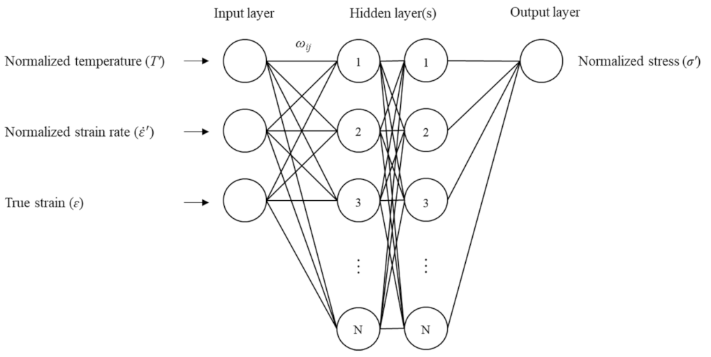
Table 1 shows the chemical composition of the A230 material. The initial rod-shaped specimen was fabricated into a diameter of 10 mm and a height of 12 mm for the compression test. Uniaxial compression tests with various strain rates were performed using a Gleeble 3800 (Dynamic System Inc., New York, NY, USA). The heating rate was set at 10 °C per second and the holding time was set at 5 min. Other compression test conditions are shown in Table 2.

2.2. ANN Model

The ANN model is an AI algorithm, and it has shown an excellent performance when solving nonlinear and complex problems [21,22,23]. Figure 1 shows the ANN structure used in this study. The input layer has three nodes. Normalized temperatures, normalized strain rates, and strains are input to each node. The reason for normalizing the temperature and strain rate values is to ensure that each of the input data have the same sensitivity in deriving a result by making the numerical ranges of each data same. The output layer has one node, and it corresponds to normalized stress values. Temperature and stress were normalized through Equation (1) and the strain rate was normalized through Equation (2). The results of normalization are presented in Table 3.
x   =   0.1   +   0.8 X     X m i n X m a x     X m i n ,
ε ˙   =   0.1   +   0.8 ln ε ˙     ln ε ˙ m i n ln ε ˙ m a x     ln ε ˙ m i n .
In order to optimize the ANN model, training was performed by varying the number of hidden layers from 4 to 12, and the number of each node from 3 to 13. For the ANN model training, flow stresses in all compression conditions with strain between 0.02 and 0.8 collected in 0.001 increments were used. In total, 12,480 datasets were applied for ANN training. In order to increase the convergence speed and stability of the model, batch normalization was applied to each hidden layer, and the resulting value was activated by the ReLU activation function. For training, the deep learning model package from TensorFlow was used. AdamOptimizer with a learning rate of 5 × 10⁻⁵ was used for optimizer. Training was performed 50,000 times with 64 mini-batch. A GEFORCE RTX 3090 GPU (NVIDIA, Santa Clara, CA, USA) was used for the training.

3. Results and Discussion

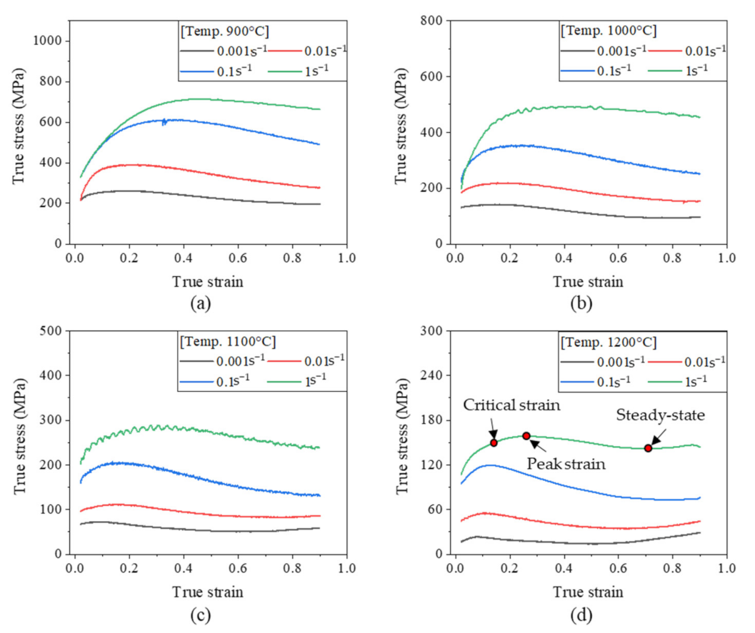
3.1. Flow Stress of A230 Alloy

Figure 2 shows the measured flow stresses for the nickel alloy A230. It can be seen that the flow stresses tended to decrease as the temperature increased and the strain rate decreased, which are general high-temperature deformation characteristics. This is because the mobility of the grain boundaries increases as the temperature increases [24,25]. The low strain rate also caused stress reduction because it provided sufficient time for the growth of DRX grains. At the initial stage of deformation, the flow stresses rapidly increased due to the work hardening for all of the deformation conditions. After the strain reached the critical strain, DRX occurred actively so that the flow stress was gradually reduced after the peak stress (Figure 2d). As a result, a steady-state in which work hardening and stress softening were balanced was observed. However, the steady state was not clearly observed when the temperature was relatively low and the strain rate was relatively high. On the other hand, when the temperature was high or the strain rate was low, secondary work hardening in which the stress increased again after the steady state was observed.

3.2. Prediction of Flow Stress

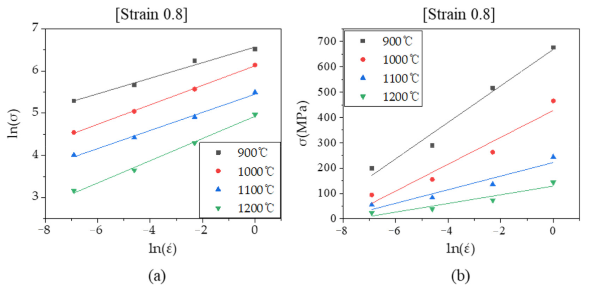
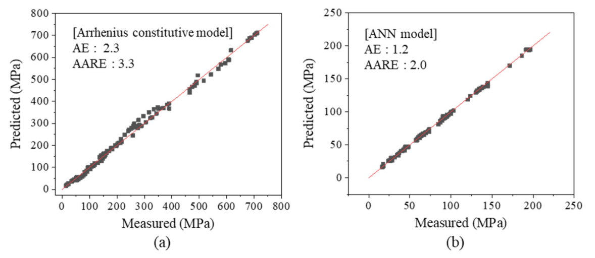
3.2.1. Arrhenius Constitutive Equation Modeling

The following Arrhenius hyperbolic sine equation has been commonly used to model the relationship between deformation conditions (temperature, strain rate) and flow stresses [26].
Z   =   ε ˙ e x p Q R T   =   C sinh α σ n ,
where, Z, ε ˙ , Q, R, T, and σ indicate the Zener–Hollomon parameter, strain rate, deformation activation energy (KJ/mol), gas constant (8.314 J/mol K), Kelvin temperature, and flow stress, respectively. C, α, and n are material constants. In ranges with high or low stress levels, the following two equations were applied for modeling [27].
Z   =   ε ˙ e x p Q R T   =   A σ n ,   α σ   <   0.8 ,
Z   =   ε ˙ e x p Q R T   =   B e x p β σ ,   α σ > 1.2 ,
where, A, B, n′, and β represent the material constants. In order to derive Equation (3), which can represent the relationship between the deformation conditions and the flow stress in all ranges, regardless of the stress level, n′ and β in Equations (4) and (5) should be obtained. The derivation process is described in detail below.
  • Calculation of n′ and β
The value of α, which is the material constant in Equation (3), is obtained by dividing β by n′. Therefore, the following equations were derived by taking the natural logarithm of both sides of Equations (4) and (5) to calculate n′ and β.
ln ε ˙   +   Q R T   =   ln A   +   n ln σ ,
ln ε ˙   +   Q R T   =   ln B   +   β σ .
n′ and β are obtained by finding the slope values of the linear fitting lines of the ln σ vs. ln ε ˙ and σ vs. ln ε ˙ graphs, respectively (Figure 3). Each n′ and β value according to temperature is averaged and used. As a result, one n′ and β value are calculated for each strain. After that, the value of α for each strain is obtained by α = β/n′.
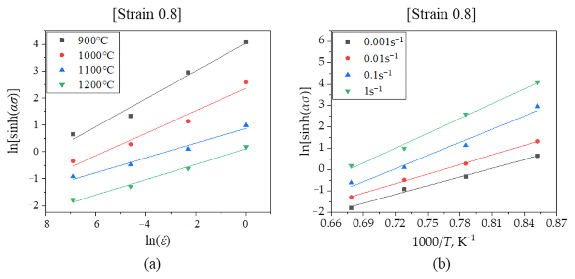
  • Calculation for n and Tp
By taking the natural logarithm of Equation (3), the following equation is obtained.
ln ε ˙   =   ln C   +   n ln sinh α σ     Q R T .
If the strain rate is constant, Equation (8) can be expressed, as below, by partial differentiation.
Q   =   R   ·   ln έ ln sinh α σ T   ·   ln sinh α σ 1 / T ε ˙ .
Figure 4 shows the linear relationship between ln[sinh(ασ)] vs. ln ε ˙ , and ln[sinh(ασ)] vs. 1000/T at strain 0.8. The value of n was obtained by averaging the slope of the linear fitting line in Figure 4a. On the other hand, in the case of Figure 4b, the Tp values according to the strain rate were used for further calculation (not averaged). This is because the strain rate dependent Tp values are more effective for predicting the flow stress [26].
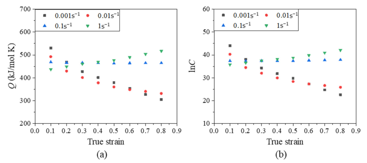
  • Calculation for Q, C and Z
By substituting the previously derived n and Tp into the equation below, the activation energy (Q) according to strain is calculated.
Q   =   R n T p ε ˙ .
In addition, the material constant C value from Equation (3) can be obtained by substituting the above Q value into the following equation. The calculated Q and C values are shown in Figure 5.
ln sinh α σ   =   ln ε ˙ n   +   Q n R T     ln C n .
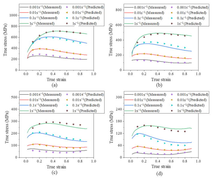
  • Flow stress prediction
By substituting the previously calculated material constants into Equation (3), the Zener–Hollomon parameters according to all temperatures, strain rates, and strains are calculated. Then, the flow stresses are calculated by substituting the Z and C values into the equation below, and the results are shown in Figure 6.
σ   =   1 α ln Z C 1 n   +   Z C 2 n   +   1 1 2 ,
As can be seen from the figure, the predicted flow stresses were similar to the measured flow stresses. However, it was observed that the difference between the predicted and measured value increased at a strain rate 0.1 s−1 under all temperature conditions. In particular, as the strain increased, the difference gradually increased. The maximum difference was calculated to be 36.14 MPa at a temperature of 900 °C, a strain rate of 0.1 s−1, and a strain of 0.8.

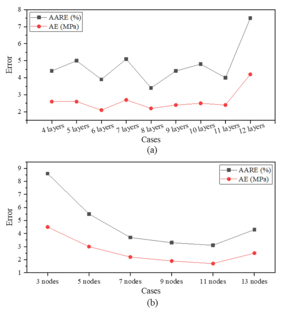
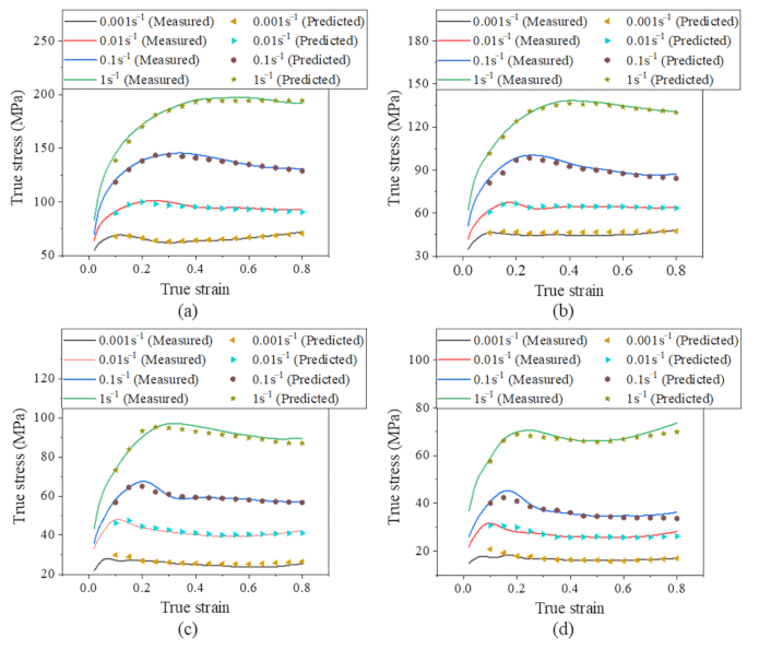
3.2.2. Result of ANN Model

As demonstrated in Section 3.2.1, the mathematical modeling of flow stresses derived based on the Arrhenius constitutive equation showed limitations in the flow stress prediction performance at high strain rates. To overcome these shortcomings, a flow stress modeling using the ANN model was applied in this study. Table 4 shows the prediction results according to a total of 54 cases in which the number of layers and nodes were different. For an accurate comparison, the absolute error (AE) and average absolute relative error (AARE) for data points of strain from 0.1 to 0.8 with increment 0.1 at all deformation conditions are calculated as follows [28].
AE   =   1 n i   =   1 n E i     P i ,
AARE   =   1 n i   =   1 n E i     P i E i   ×   100 ,
where, Ei, Pi, and n indicate measured stress, predicted stress, and the number of data points, respectively.
To ease the comparison, graphs showing the accuracy according to the number of hidden layers and nodes are shown in Figure 7. As can be seen from Figure 7a, no significant tendency according to the number of hidden layers was observed. However, when 12 hidden layers were used, both AARE and AE increased dramatically (it is noted here that the lower accuracy was measured when one to three hidden layers were applied). It is considered that this is because too many hidden layers cause an over-fitting problem. Therefore, it is determined that the use of the six hidden layers is the optimal number of layers based on the AE results. On the other hand, it can be seen that the number of nodes greatly affects the prediction ability (Figure 7b). The lowest AARE and AE were measured at the case of 11 nodes. Therefore, it can be concluded that the optimal ANN structure is to use 6 hidden layers with 11 nodes for modeling the relationship between deformation conditions and flow stresses.
Graphs comparing the predicted and measured flow stresses using the optimized ANN model (6 layers with 11 nodes) are shown in Figure 8. As can be seen from the figure, the predicted values were in good agreement with the measured values under the entire strain condition. In addition, the accuracy reduction at a strain rate of 1 s−1, which was the limitation of the Arrhenius constitutive equation, did not exist when the ANN model was used.
Figure 9 shows the correlation between the measured and predicted values. In the case of the Arrhenius constitutive equation model, the error increased near the stress of 300 MPa. On the other hand, the ANN model predicted stress accurately over the entire stress range. The AE and AARE values for the entire evaluation data were calculated as 1.2 and 2.0 for the ANN model, and 2.3 and 3.3 for the Arrhenius constitutive equation model, respectively. Therefore, it can be confirmed that the ANN model exhibited a more accurate performance for predicting flow stresses.

4. Conclusions

In this study, the flow stress characteristics at high temperature deformation for the A230 material were analyzed using mathematical modeling and AI technology. First, based on the flow stresses measured by the Gleeble test, the flow stresses at various strain rates and temperatures were modeled using the Arrhenius constitutive equation and the ANN model. Based on the evaluation metrics, they were calculated as AE 1.2 and AARE 2.0 for the ANN model, and AE 2.3 and AARE 3.3 for the Arrhenius constitutive equation, respectively. Accordingly, it was confirmed that AI technology showed better results in modeling the complex relationship between the process conditions and flow stresses.

Author Contributions

Conceptualization, I.Y.M. and H.W.J.; methodology, H.W.L.; software, S.-J.K.; validation, Y.-S.O. and J.J.; formal analysis, S.O.; investigation, I.Y.M.; resources, S.O.; data curation, S.-H.K.; writing—original draft preparation, I.Y.M.; writing—review and editing, S.-H.K.; visualization, S.O.; supervision, S.-H.K.; project administration, H.W.L.; funding acquisition, H.W.J. All authors have read and agreed to the published version of the manuscript.

Funding

This work was supported by the Technology Innovation Program (project no. 20011444 and project no. N0002598) funded by the Ministry of Trade, Industry, and Energy (MOTIE, Korea).

Institutional Review Board Statement

Not applicable.

Informed Consent Statement

Not applicable.

Data Availability Statement

All the codes and the training data required to reproduce our works are available from the corresponding author on reasonable request.

Conflicts of Interest

The authors have no financial or proprietary interest in any material discussed in this article.

References

  1. Chen, F.; Cui, Z.; Chen, S. Recrystallization of 30Cr2Ni4MoV ultra-super-critical rotor steel during hot deformation. Part I: Dynamic recrystallization. Mater. Sci. Eng. A 2011, 528, 5073–5080. [Google Scholar] [CrossRef]
  2. Lv, B.J.; Peng, J.; Shi, D.W.; Tang, A.T.; Pan, F.S. Constitutive modeling of dynamic recrystallization kinetics and processing maps of Mg–2.0 Zn–0.3 Zr alloy based on true stress–strain curves. Mater. Sci. Eng. A 2013, 560, 727–733. [Google Scholar] [CrossRef]
  3. Yang, Q.; Ji, C.; Zhu, M. Modeling of the dynamic recrystallization kinetics of a continuous casting slab under heavy reduction. Metall. Mater. Trans. A 2019, 50, 357–376. [Google Scholar] [CrossRef]
  4. Kumar, S.S.; Raghu, T.; Bhattacharjee, P.P.; Rao, G.A.; Borah, U. Work hardening characteristics and microstructural evolution during hot deformation of a nickel superalloy at moderate strain rates. J. Alloy. Compd. 2017, 709, 394–409. [Google Scholar] [CrossRef]
  5. Xu, Y.; Hu, L.; Sun, Y. Deformation behaviour and dynamic recrystallization of AZ61 magnesium alloy. J. Alloy. Compd. 2013, 580, 262–269. [Google Scholar] [CrossRef]
  6. Xu, D.; Zhu, M.; Tang, Z.; Sun, C. Determination of the dynamic recrystallization kinetics model for SCM435 steel. J. Wuhan Univ. Technol. Mater. Sci. Ed. 2013, 28, 819–824. [Google Scholar] [CrossRef]
  7. Rajput, S.K.; Chaudhari, G.P.; Nath, S.K. Characterization of hot deformation behavior of a low carbon steel using processing maps, constitutive equations and Zener-Hollomon parameter. J. Mater. Process. Technol. 2016, 237, 113–125. [Google Scholar] [CrossRef]
  8. Liu, Y.; Hu, R.; Li, J.; Kou, H.; Li, H.; Chang, H.; Fu, H. Deformation characteristics of as-received Haynes230 nickel base superalloy. Mater. Sci. Eng. A 2008, 497, 283–289. [Google Scholar] [CrossRef]
  9. Ji, H.; Cai, Z.; Pei, W.; Huang, X.; Lu, Y. DRX behavior and microstructure evolution of 33Cr23Ni8Mn3N: Experiment and finite element simulation. J. Mater. Res. Technol. 2020, 9, 4340–4355. [Google Scholar] [CrossRef]
  10. Poletti, C.; Six, J.; Hochegger, M.; Degischer, H.P.; Ilie, S. Hot deformation behaviour of low alloy steel. Steel Res. Int. 2011, 82, 710–718. [Google Scholar] [CrossRef]
  11. Chen, X.M.; Lin, Y.C.; Wen, D.X.; Zhang, J.L.; He, M. Dynamic recrystallization behavior of a typical nickel-based superalloy during hot deformation. Mater. Des. 2014, 57, 568–577. [Google Scholar] [CrossRef]
  12. Lin, Y.C.; Chen, M.S.; Zhong, J. Prediction of 42CrMo steel flow stress at high temperature and strain rate. Mech. Res. Commun. 2008, 35, 142–150. [Google Scholar] [CrossRef]
  13. Torquato, S.; Haslach, H.W., Jr. Random heterogeneous materials: Microstructure and macroscopic properties. Appl. Mech. Rev. 2002, 55, B62–B63. [Google Scholar] [CrossRef]
  14. Yang, Z.; Yabansu, Y.C.; Jha, D.; Liao, W.K.; Choudhary, A.N.; Kalidindi, S.R.; Agrawal, A. Establishing structure-property localization linkages for elastic deformation of three-dimensional high contrast composites using deep learning approaches. Acta Mater. 2019, 166, 335–345. [Google Scholar] [CrossRef]
  15. Cang, R.; Li, H.; Yao, H.; Jiao, Y.; Ren, Y. Improving direct physical properties prediction of heterogeneous materials from imaging data via convolutional neural network and a morphology-aware generative model. Comput. Mater. Sci. 2018, 150, 212–221. [Google Scholar] [CrossRef] [Green Version]
  16. Iyer, A.; Dey, B.; Dasgupta, A.; Chen, W.; Chakraborty, A. A conditional generative model for predicting material microstructures from processing methods. arXiv 2019, arXiv:1910.02133. [Google Scholar]
  17. Lee, J.W.; Goo, N.H.; Park, W.B.; Pyo, M.; Sohn, K.S. Virtual microstructure design for steels using generative adversarial networks. Eng. Rep. 2021, 3, e12274. [Google Scholar] [CrossRef]
  18. Shouwu, G.; Leina, Z. A comparison study at the flow stress prediction of Ti-5Al-5Mo-5V-3Cr-1Zr alloy based on BP-ANN and Arrhenius model. Mater. Res. Express 2018, 5, 066505. [Google Scholar] [CrossRef]
  19. Liu, J.; Chang, H.; Hsu, T.Y.; Ruan, X. Prediction of the flow stress of high-speed steel during hot deformation using a BP artificial neural network. J. Mater. Process. Technol. 2000, 103, 200–205. [Google Scholar] [CrossRef]
  20. Sani, S.A.; Ebrahimi, G.R.; Vafaeenezhad, H.; Kiani-Rashid, A.R. Modeling of hot deformation behavior and prediction of flow stress in a magnesium alloy using constitutive equation and artificial neural network (ANN) model. J. Magnes. Alloy. 2018, 6, 134–144. [Google Scholar] [CrossRef]
  21. Moon, I.Y.; Lee, H.W.; Kim, S.J.; Oh, Y.S.; Jung, J.; Kang, S.H. Analysis of the Region of Interest According to CNN Structure in Hierarchical Pattern Surface Inspection Using CAM. Materials 2021, 14, 2095. [Google Scholar] [CrossRef] [PubMed]
  22. Jha, R.; Dulikravich, G.S. Discovery of new Ti-based alloys aimed at avoiding/minimizing formation of α” and ω-phase using CALPHAD and artificial intelligence. Metals 2021, 11, 15. [Google Scholar] [CrossRef]
  23. Jedamski, R.; Epp, J. Non-destructive micromagnetic determination of hardness and case hardening depth using linear regression analysis and artificial neural networks. Metals 2021, 11, 18. [Google Scholar] [CrossRef]
  24. Lee, H.W.; Im, Y.T. Numerical modeling of dynamic recrystallization during nonisothermal hot compression by cellular automata and finite element analysis. Int. J. Mech. Sci. 2010, 52, 1277–1289. [Google Scholar]
  25. Jung, K.H.; Lee, H.W.; Im, Y.T. Numerical prediction of austenite grain size in a bar rolling process using an evolution model based on a hot compression test. Mater. Sci. Eng. A 2009, 519, 94–104. [Google Scholar] [CrossRef]
  26. Wang, L.; Liu, F.; Cheng, J.J.; Zuo, Q.; Chen, C.F. Arrhenius-type constitutive model for high temperature flow stress in a Nickel-based corrosion-resistant alloy. J. Mater. Eng. Perform. 2016, 25, 1394–1406. [Google Scholar] [CrossRef]
  27. Wei, H.L.; Liu, G.Q.; Xiao, X.; Zhang, M.H. Dynamic recrystallization behavior of a medium carbon vanadium microalloyed steel. Mater. Sci. Eng. A 2013, 573, 215–221. [Google Scholar] [CrossRef]
  28. Wan, P.; Zou, H.; Wang, K.; Zhao, Z. Research on hot deformation behavior of Zr-4 alloy based on PSO-BP artificial neural network. J. Alloy. Compd. 2020, 826, 154047. [Google Scholar] [CrossRef]
Figure 1. Architecture of the ANN used to predict the flow stress curves.
Metals 12 00223 g001
Figure 2. A230 flow stress curves measured at (a) 900, (b) 1000, (c) 1100 and (d) 1200 °C.
Metals 12 00223 g002
Figure 3. Calculation of the value of (a) n′ by plotting ln σ vs. ln ε ˙ and (b) β by plotting σ vs. ln ε ˙ . All values correspond to strain 0.8.
Metals 12 00223 g003
Figure 4. Calculation of the value of (a) n by plotting ln[sinh(ασ)] vs. ln ε ˙ and (b) Tp by plotting ln[sinh(ασ)] vs. 1000/T. All values correspond to strain 0.8.
Metals 12 00223 g004
Figure 5. Calculated material constants of (a) deformation activation energy and (b) ln C.
Metals 12 00223 g005
Figure 6. Experimental and predicted flow stress curves using the Arrhenius constitutive model for (a) 900, (b) 1000, (c) 1100, and (d) 1200 °C.
Metals 12 00223 g006
Figure 7. Graphs depicting the results of AARE and AE calculation according to (a) the number of hidden layers and (b) the number of nodes.
Metals 12 00223 g007
Figure 8. Experimental and predicted flow stress curves using the ANN model for (a) 900, (b) 1000, (c) 1100, and (d) 1200 °C.
Metals 12 00223 g008
Figure 9. Correlation relationships between the measured and predicted values using the (a) Arrhenius constitutive model and (b) ANN model.
Metals 12 00223 g009
Table 1. Chemical composition of the A230 material.
MaterialChemical Composition (wt%)
A230FeMnSiCrCAlNbCoTiMoLaBWNi
30.50.4220.10.30.550.120.020.0214Bal.
Table 2. Experimental parameters for the Gleeble test.
Conditions
Temperature (°C) Strain Strain Rate (s−1)
900, 1000, 1100, 1200~0.90.001, 0.01, 0.1, 1
Table 3. Summary of normalized input and output data.
Data StatesInputOutput
TemperatureStrain RateStrainStress
Range of
raw data
900–1200 °C0.001–1 s−10.1–0.915–240 MPa
Range of
normalized data
0.1–0.90.1–0.90.1–0.90.1–0.9
Table 4. Results of the ANN prediction according to the number of layers and nodes.
CaseNo.
Layers
No. NodesAE
(MPa)
AARE
(%)
CaseNo.
Layers
No. NodesAE
(MPa)
AARE
(%)
1435.09.028891.62.3
252.94.629111.62.0
372.54.230131.72.6
492.33.631935.19.1
5111.32.43252.75.9
6131.52.53371.93.9
7535.710.03491.42.1
852.75.235111.42.4
971.93.136131.63.2
1092.04.0371035.210.1
11111.32.93853.77.1
12132.25.03972.03.5
13633.15.84091.63.2
1453.47.341111.52.6
1571.83.642131.12.6
1691.82.9431134.16.3
17111.22.04452.84.5
18131.22.04572.13.4
19734.511.74691.93.2
2053.35.247112.04.6
2172.84.348131.22.1
2291.62.8491235.110.4
23112.03.45052.84.2
24131.93.55172.54.4
25833.04.75292.65.3
2653.05.353112.85.2
2772.33.454139.615.4
Publisher’s Note: MDPI stays neutral with regard to jurisdictional claims in published maps and institutional affiliations.

