Article

Thermodynamic Simulation of Solidification of Ti-Containing Steels with Consideration for Possibility of Peritectic Transformation and Second Phase Precipitation

M.N. Mikheev Institute of Metal Physics of Ural Branch of Russian Academy of Sciences, Ekaterinburg 620108, Russia
*
Author to whom correspondence should be addressed.
Submission received: 16 November 2022 / Revised: 15 December 2022 / Accepted: 20 December 2022 / Published: 23 December 2022

Abstract

:
An algorithm is proposed for predicting the phase composition of titanium-containing steels after solidification. The approach is based on thermodynamic calculations and provides for crystallization through the formation of ferrite and austenite, as well as a peritectic reaction. The algorithm takes into account the possibility of precipitation of TiN, TiS, MnS and TiC0.5S0.5 from the liquid phase upon crystallization. Two possible behaviors of ferrite upon crystallization are considered: frozen and fast diffusion of elements in the metal sublattice of this phase. Calculations illustrating the operation of the proposed algorithm have been performed.

1. Introduction

Several methods are used to simulate the crystallization of steels. The authors of some of them try to solve the problem in the most general form, taking into account diffusion and motion of phase boundaries, as, for example, in the DICTRA module of the Thermo-Calc program [1] or the IDS program [2]. As a variation of this approach, the cellular automation method can be used to describe the motion of phase boundaries [3]. An essential advantage of these approaches is the possibility of predicting the structure of steels (although only in 2D in the case of using cellular automation). However, this requires highly resource-intensive algorithms, and the authors must use significant simplifications and assumptions in order to complete the simulation in an acceptable time. There are also attempts to use machine learning in this area [4,5].
Consideration of the peritectic transformation during solidification is particularly difficult. According to a review of various aspects of peritectic transformation given in [6], peritectic steel solidification occurs in two distinct stages liquid (L), delta-ferrite (δ), and austenite (γ): the peritectic reaction (δ + L → γ) followed by the peritectic transformation (δ → γ). However, it is noted in [6] that there is also disagreement regarding the peritectic transformation: some believe that peritectic transformation is diffusion controlled while others believe that massive transformation is responsible for this phenomenon.
Up to now, an approach based on thermodynamic calculations remains popular since it allows, at relatively low computational costs, to estimate the temperature range of crystallization of an alloy and its final phase composition. Traditionally, such calculations are carried out in the Sheil–Gulliver (SG) approximation [7,8] or the lever rule (LR). In the SG model, it is assumed that diffusion in the solidificated portions of solid phases is “frozen”, while in the liquid phase, it, on the contrary, is infinitely fast. Thermodynamic equilibrium is established between the liquid and the next portion of the solid phase. In the case of using the approximation of the lever rule, complete equilibrium between all the present phases is assumed. However, real alloys often contain both substitution elements (slowly diffusing) and interstitial elements (fast diffusing), so neither one nor the other approximation is completely suitable for them.
To solve this problem, approximations of partial and para-equilibrium were proposed [9,10]. The first assumes rapid diffusion of interstitial elements in the solid phase and frozen diffusion of substitutional elements. This condition is expressed as the equality of chemical potentials of interstitial elements (for example, C) in the liquid (L) and solid (S) phases:
μ C L = μ C S
The para-equilibrium between f1 and f2 phases is supplemented by the condition:
i u i f 1 μ i f 1 = i u i f 2 μ i f 2 ,   where   i Me .
Here u i f 1 is a concentration variable calculated as:
u i f 1 = X i f 1 / j X j f 1 ,   where   j Me .
Here X i f i is mole fraction of the i-th element in fi phase. The designation “ Me ” means “relating to metal sublattice (substitution sublattice)”.
Approximations of partial and para-equilibrium were successfully implemented in a number of algorithms and software products [11,12,13,14]. The partial equilibrium approximation was also used in a recent publication [15]. The algorithm presented in this paper is largely based on these works, but the authors believe it offers a better solution in some respects. Firstly, most of the algorithms presented to date take into account only the accelerated diffusion of carbon but do not consider the fact that nitrogen, which is usually present in steels, also rapidly diffuses in the interstitial sublattice. Secondly, many of the proposed models are aimed only at determining the temperature range of crystallization and do not consider the formation of excess phases upon melt solidification. Thirdly, it seems strange to use the para-equilibrium approximation, as, for example, in [12] to describe the peritectic transformation, since the derivation of condition (2) uses an assumption that concentrations of elements in a substitution sublattice are equal for the phases in para-equilibrium [9,16], which is obviously not the case for austenite and ferrite. Finally, for those algorithms that are quite well described in [11,12], in the flowchart, one can see additional steps for partial and/or para-equilibrium. In the algorithm proposed here, the peritectic transformation is simulated in one step, which is both more convenient and more consistent with the formulation of the peritectic reaction from the thermodynamic viewpoint (δ + L → γ + L).

2. Model Description

The model is implemented as a program for predicting the phase composition of titanium-containing steels after solidification. In addition to Ti, the presence of C, N, Cr, Mn, Si and S elements in the alloy and the possibility of precipitation of TiN, TiC0.5S0.5, TiS and MnS phases are taken into account. Simulation is carried out based on a step-by-step procedure, i.e., at each temperature step, the current temperature value decreases by ΔT, and the system state corresponding to the new temperature is calculated. To start the calculations, the temperature is set a few degrees higher than the highest of the temperatures: the beginning of solidification or the beginning of the precipitation of excess phases.
The temperatures of beginning of these compounds precipitation from the melt were calculated based on the temperature dependences of their equilibrium constants with the melt according to the following formulas (for compound AB):
l g K AB = l g a A L a B L a AB = f T
Here f(T) is the function of temperature. The activities of the reaction products a AB were taken equal to unity. Activities of titanium ( a Ti ), nitrogen ( a N ), carbon ( a C ), manganese ( a Mn ) and sulfur ( a S ) in the melt were calculated using formulas:
l g a A L = l g % A L + i e A i L % i L
where % A L is concentration of element A in the melt, and e A i L are coefficients of elements interaction in the melt. Subsequently, at each temperature step, the amounts of precipitated phases Q T i N , Q M n S , Q T i S and Q T i C 0.5 S 0.5 were determined from the solution of the system of Equations (4) and (5).
The temperatures of the beginning of ferrite and austenite formation in the first approximation were estimated from the formulas obtained based on the analysis of the state diagrams of binary systems:
T L δ = 1811 75.685 % C L 11.718 % C L 2 4.8 % Mn L 11.4 % Si L 14.3 % S L ,         K
T L γ = 1796.3 49.51 % C L 8.247 % C L 2 4.8 % Mn L 11.4 % Si L 13.3 % S L ,         K
The values T L δ and T L γ determined by expressions (6) and (7), are used as the first approximation for a more accurate calculation by solving the system of equations (described in detail below, see (8)–(12), as well as an additional condition for equal to zero fraction of ferrite or austenite. If it turns out that T L δ > T L γ , then the algorithm simulates crystallization according to the “ferrite scenario”, i.e., with precipitation of ferrite from the liquid phase, and also tries to calculate the peritectic transformation at each temperature step. If T L δ < T L γ , then there is certainly no peritectic transformation, and the calculation proceeds according to the “austenitic scenario”.
At each k-th temperature step, mass fractions of the liquid phase Q L k , ferrite Q δ k and/or austenite Q γ k , were calculated, as well as the changes in the composition of the melt and solid phases. The calculation can be carried out based on the “frozen” diffusion approximation in the metal sublattice of ferrite and austenite and in the approximation of infinitely fast diffusion in the metal sublattice of ferrite (with frozen diffusion of substitutional elements in austenite), as suggested, for example, in [13].
Two sets of equations were used to describe the formation of δ-ferrite and/or austenite: for the first appearance of a solid phase and for the ongoing appearance (when this solid phase has already appeared at previous temperature steps).

2.1. Approximation of Frozen Diffusion in Metal Sublattices of All Crystalline Phases

The set of equations used for austenite crystallization is the same as for ferrite crystallization. Therefore, the following equations are given only for the “ferrite scenario”.

2.1.1. The Appearance of the First Portion of Ferrite (dδ) upon Crystallization from the Liquid Phase without (before) Peritectic Transformation

Variables: % i L k , % i d δ k , Q L k , Q d δ k are concentrations of elements in the liquid phase and the first portion of ferrite and mass fractions of the liquid phase and the first portion of ferrite—total 2n + 2 variables, where n is the number of alloying elements.
Equations:
Mass balance over all alloying elements (n equations):
% C L k Q L k + % C d δ k Q d δ k + % C TiC 0.5 S 0.5 k 1 = C C ,
% N L k Q L k + % N d δ k Q d δ k + % N TiN k 1 = C N ,
% i L k Q L k + % i d δ k Q d δ k = % i L k 1 Q L k 1 ,   where   i C , N .
Here CC and CN are the amounts of C and N in the alloy.
It is assumed that a small portion of the newly formed solid phase has a complete equilibrium composition with respect to the liquid phase. This corresponds to the condition of equality of chemical potentials of all elements, including Fe, between the liquid and a new portion of δ-ferrite (n + 1 equations):
μ i L = μ i d δ
Equality to unity of the sum of phase fractions (1 equation):
Q L k + Q d δ k + i Q p r e c i k = 1 ,
where i Q p r e c i k is the sum of second phase fractions.
Starting points. As starting points for the liquid phase composition, the alloy composition is taken minus amount of the elements that, by this temperature, have already turned out to be bound in TiN, TiC0.5S0.5, TiS and MnS, that is, in fact, the composition of the melt, which corresponds to a given temperature step: % i L 0 k = % i L k . For the starting points of the δ-ferrite composition, one can use coefficients of elements distribution between the liquid and ferrite, w i L , which can be roughly calculated in advance from binary phase diagrams or based on any thermodynamic calculations:
% i d δ 0 k = w i L δ % i L 0 k ,
Some small value Δδ can be taken as the starting value of δ-ferrite fraction. The increment of the solid phase fraction obviously depends on the temperature step. For example, for ΔT = 0.01, one can use Q δ 0 k = 0.001 . Accordingly, for the liquid phase, Q L 0 k = 1 Δ δ .

2.1.2. Continued Appearance of Ferrite upon Crystallization from Liquid Phase without (before) Peritectic Transformation

Variables: % i L k , Y C δ k , Y N δ k , % i d δ k , Q L k , Q δ k , Q d δ k —total 2n + 4.
Here Y C δ k and Y N δ k are mole fractions of C and N in interstitial sublattice of ferrite. The mole fraction of the i-th element in f phase is related to concentrations of elements in sublattices as:
X i f = s = 1 l a s Y i f s s = 1 l a s 1 Y va f s ,
where a s is the number of sites on the sublattice s per mole of formula units of the phase. For austenite, a 1 = 1 , a 2 = 1 ; and for ferrite, a 1 = 1 , a 2 = 3 . Y va f s is the mole fraction of structural vacancies in sublattice s.
Mole fractions of elements in a phase are related to mass fractions by known ratios.
Y C δ k and Y N δ k act as variables since it is assumed that C and N are freely redistributed among all solid phases, including the previously formed ferrite. The Y values of metal elements in the previously formed ferrite are taken equal to those obtained at the previous temperature step. Thus, having a complete set of mole fractions of components in both ferrite sublattices, it is possible to calculate the molar and, accordingly, mass fractions of elements in the previously formed ferrite, which are obtained at a given iteration of solving the system of equations.
The mass fraction of earlier formed ferrite is calculated from the condition of mass conservation of any metal element in ferrite at the previous and new time steps:
Q δ k = Q δ k 1 % i δ k 1 % i δ k ,   where   i Me .
Equations:
Mass balance over all alloying elements (n equations)
% C L k Q L k + % C δ k Q δ k + % C d δ k Q d δ k + % C TiC 0.5 S 0.5 k 1 = C C ,
% N L k Q L k + % N δ k Q δ k + % N d δ k Q d δ k + % N TiN k 1 = C N ,
% i L k Q L k + % i d δ k Q d δ k = % i L k 1 Q L k 1 ,   where   i C , N .
The approximation of partial equilibrium was used, that is, for carbon and nitrogen, equilibrium was assumed between the liquid, the new portion and the previously formed δ-ferrite, and for the rest of the elements, only between the melt and the next portion of δ-ferrite (n + 3 equations):
μ i L = μ i d δ
μ i L = μ i δ ,   where   i C , N .
The sum of phase fractions is equal to 1 (1 equation):
Q L k + Q δ k + Q d δ k + i Q p r e c i k = 1 .
Starting points. As starting points for the liquid phase composition, its composition obtained at the previous temperature step is taken: % i L 0 k = % i L k 1 . Analogously, for δ-ferrite composition: Y C γ 0 k = Y C γ k 1 , Y N γ 0 k = Y N γ k 1 and % i d γ 0 k = % i γ k 1 . For fractions of phases: Q L 0 k = Q L k 1 Δ δ , Q δ k = Q δ k 1 , Q d δ k = Δ δ .

2.1.3. First Occurrence of Austenite ( d γ ) upon Peritectic Transformation

Variables: % i L k , Y C δ k , Y N δ k , % i d γ k   Q L k , Q δ k , Q d γ k —total 2n + 5 variables.
Since the metallic elements from the previously formed ferrite in this case no longer remain there, but also partially transfer into the newly appeared austenite, the mass fraction of ferrite can no longer be calculated from the condition of mass conservation of any metallic element in ferrite, as in (15). Therefore, the fraction of ferrite at the new temperature step is an independent variable.
Similarly to the case of simple crystallization, the Y-s of metal elements in the previously formed ferrite are taken equal to those obtained at the previous temperature step. And, taking into account variables Y C δ k and Y N δ k , the atomic and mass fractions of elements in the previously formed ferrite are calculated, which will be obtained at this iteration of solving the system of equations, respectively.
Equations:
Mass balance for all doping elements (n equations):
% C L k Q L k + % C δ k Q δ k + % C d γ k Q d γ k + % C TiC 0.5 S 0.5 k 1 = C C ,
% N L k Q L k + % N δ k Q δ k + % N d γ k Q d γ k + % N TiN k 1 = C N ,
% i L k Q L k + % i δ k Q δ k + % i d γ k Q d γ k = % i L k 1 Q L k 1 + % i δ k 1 Q δ k 1 ,   where   i C , N .
Equality of chemical potentials of all elements, including Fe, in the liquid and a new portion of austenite (n + 1 equations):
μ i L = μ i d γ ,
Equality of chemical potentials of C and N in the liquid phase and previously formed ferrite (2 equations):
μ i L = μ i δ ,   where   i C , N .
Partial equilibrium established between the previously formed ferrite and other phases, in particular, liquid, is a special case of equilibrium. Consequently:
Δ G = G δ i X i δ μ i L = i X i δ μ i δ i X i δ μ i L = 0 .
This condition can be somewhat simplified. Taking into account the equality of chemical potentials of C and N:
i X i δ μ i δ i X i δ μ i L = 0 ,   where   i C , N .
and, if divided by 1 X C δ X N δ , then:
i U i δ μ i δ μ i L = 0 ,   where   i C , N .
and the last equation—the sum of phase fractions is equal to 1:
Q L k + Q δ k + Q d γ k + i Q p r e c i k = 1
Starting points: % i L 0 k = % i L k 1 , Y C δ 0 k = Y C δ k 1 , Y N δ 0 k = Y N δ k 1 . Composition of the new portion of austenite % i d γ k can be calculated by an expression analogous to (13). For phase fractions: Q L 0 k = Q L k 1 Δ γ , Q δ k = Q δ k 1 , Q d γ k = Δ γ , where Δ γ is the value an order of Δ δ .

2.1.4. Continued Appearance of Austenite upon Peritectic Transformation

Variables: % i L k , Y C δ k , Y N δ k , Y C γ k , Y N γ k , % i d γ k   Q L k , Q δ k , Q d γ k —total 2n + 7.
Similarly to the above-considered cases, it is assumed that the composition of metal sublattices in ferrite and austenite formed earlier does not change, while C and N can fluently diffuse in them, establishing an equilibrium concentration. Thus, taking into account variables Y C δ k , Y N δ k , Y C γ k and Y N γ k at each iteration step of solving the system of equations, the concentrations of all elements in the sublattices of these phases are known, and their composition can be calculated in molar and mass fractions.
Just as in the case of ferrite crystallization without peritectic transformation, the mass fraction of austenite precipitated earlier at a new temperature step can be calculated as:
Q γ k = Q γ k 1 % i γ k 1 % i γ k ,   where   i Me .
Equations:
Mass balance for all doping elements (n equations)
% C L k Q L k + % C δ k Q δ k + % C γ k Q γ k + % C d γ k Q d γ k + % C TiC 0.5 S 0.5 k 1 = C C ,
% N L k Q L k + % N δ k Q δ k + % N γ k Q γ k + % N d γ k Q d γ k + % N TiN k 1 = C N ,
% i L k Q L k + % i δ k Q δ k + % i d γ k Q d γ k = % i L k 1 Q L k 1 + % i γ k 1 Q δ k 1 ,   where   i C , N .
Equality of chemical potentials of all elements, including Fe, in the liquid and a new portion of austenite (n + 1 equations):
μ i L = μ i d γ ,  
Equality of chemical potentials of C and N in the liquid phase, previously formed ferrite and austenite (4 equations):
μ i L = μ i δ = μ i γ ,   where   i C , N .
The equilibrium condition between the liquid phase and the previously formed ferrite (1 equation):
i U i δ μ i δ μ i L = 0 ,   where   i C , N .
The sum of phase fractions is equal to 1 (1 equation):
Q L k + Q δ k + Q γ k + Q d γ k + i Q p r e c i k = 1 .
Starting points: % i L 0 k = % i L k 1 , Y C δ 0 k = Y C δ k 1 , Y N δ 0 k = Y N δ k 1 , Y C γ 0 k = Y C γ k 1 , Y N γ 0 k = Y N γ k 1 , % i d γ 0 k = % i γ k 1 , Q L 0 k = Q L k 1 Δ γ , Q γ k = Q γ k 1 , Q d γ k = Δ γ . .

2.2. Approximation of Fast Diffusion in Ferrite Metal Sublattice

2.2.1. Crystallization of Ferrite from the Liquid Phase without (up to) Peritectic Transformation

Fast diffusion in the ferrite metal sublattice provides complete equilibrium redistribution of all elements (not only C and N) in the phases. In this case, both the appearance of the first portion of crystallized ferrite and all subsequent ones is calculated based on the set of equations presented in Section 2.1.1.

2.2.2. First Occurrence of Austenite upon Peritectic Transformation

Variables: % i L k , % i δ k , % i d γ k   Q L k , Q γ k , Q d γ k total 3n + 3.
Equations:
Mass balance for all doping elements (n equations)
% i L k Q L k + % i δ k Q δ k + % i d γ k Q d γ k = % i L k 1 Q L k 1 + % i δ k 1 Q δ k 1 .
Equality of chemical potentials of all elements, including Fe, in the liquid, ferrite and a new portion of austenite (2n + 2 equations):
μ i L = μ i δ = μ i d γ .
Equality to unity of the sum of phase fractions—1 equation, the same as (30).
Starting points for all cases when using the fast diffusion approximation in the ferrite substitution sublattice are chosen in the same way as for the case of frozen diffusion considered above.

2.2.3. Continued Appearance of Austenite under Peritectic Transformation
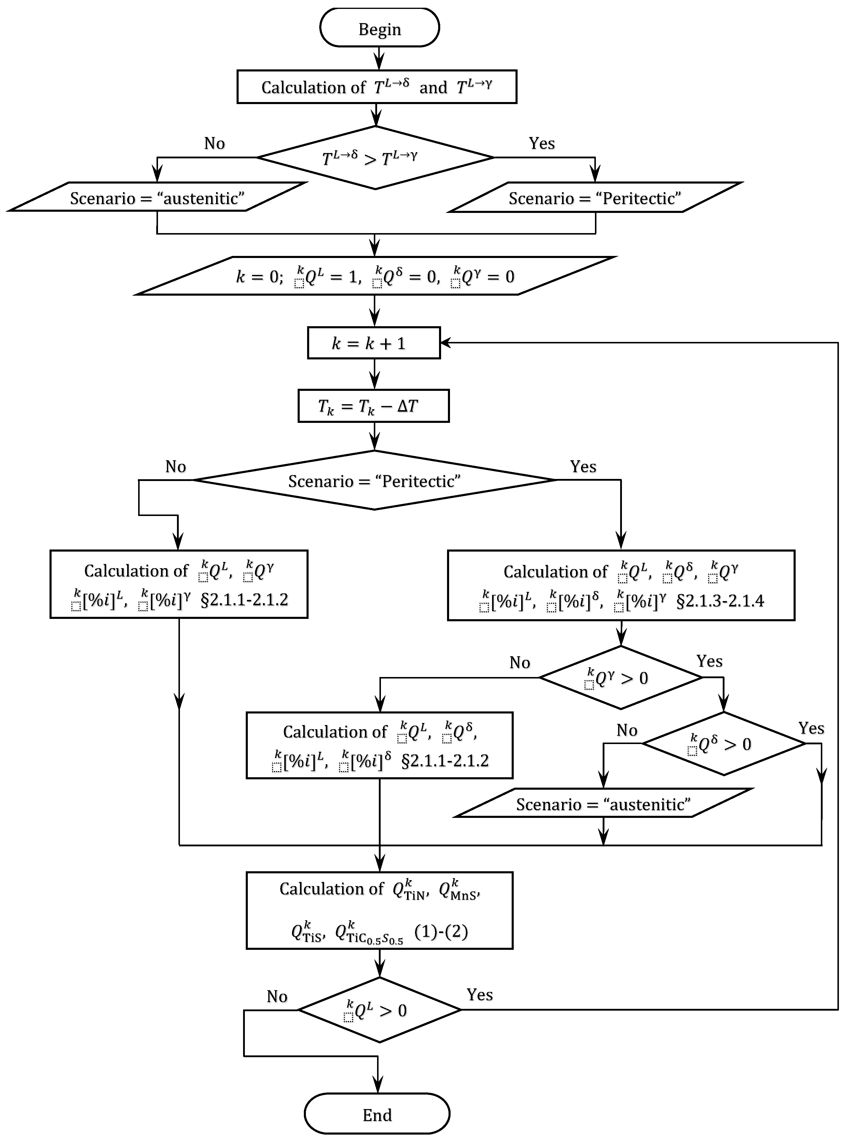
Variables: % i L k , % i δ k , Y C γ k , Y N γ k , % i d γ k   Q L k , Q δ k , Q d γ k —total 3n + 5.
Equations:
Mass balance for all doping elements (the same n equations as (39)).
Equality of chemical potentials of all elements, including Fe, in liquid, ferrite and a new portion of austenite (2n + 2 equations, as in (40)).
The equality of the chemical potentials of C and N in the liquid phase and the previously formed austenite (2 equations):
μ i L = μ i γ ,   where   i C , N .
Equality to unity of the sum of phase fractions—1 equation, the same as (38).

2.3. Algorithm

The algorithm scheme is shown in Figure 1. If the austenite appearance temperature calculated before the start of the main part of the algorithm turns out to be higher than the ferrite appearance temperature, then crystallization will follow the “austenitic scenario”. In this case, at each temperature step, the composition and amounts of the liquid phase and austenite are determined by the formulas given in Section 2.1.1 and Section 2.1.2, and the amount of elements bound in TiN, TiC0.5S0.5, TiS and MnS is determined by Equations (4) and (5).
If it turns out that T L δ < T L γ , then there is a possibility of peritectic transformation. Therefore, at each temperature step, an attempt is made to calculate the three-phase equilibrium state Liquid + δ + dγ. If the current attempt appears unsuccessful (it is considered successful if 0 < Q L k ,   Q δ k , Q d γ k < 1 ), then the composition and amount of the liquid phase and δ-ferrite are calculated according to the formulas given in Section 2.1.1 and Section 2.1.2. If the peritectic transformation has begun, then it continues as long as δ-ferrite remains in the system (condition Q δ k > 0 in Figure 1). If δ-ferrite disappears ahead of the liquid phase, then the calculation proceeds according to the “austenitic scenario”. If the entire liquid solidifies before the disappearance of the δ-ferrite, then the algorithm completes its work.

3. Model Parameters

The main goal of this work is to present the calculation algorithm. The choice of good parameter values for some alloys is a separate complicated task. Therefore, only a brief list of parameters used in the software implementation of this algorithm is given below.
The values of the equilibrium constants, except for the solubility product of titanium carbosulfide, and the coefficients of interaction of elements in the melt were used the same as in a recent publication [15]. The solubility product of carbosulfide in the melt was calculated based on the solubility product of this compound in austenite presented in [17], and the following expression was obtained:
lg % T i % C 0.5 % S 0.5 = 16317 T + 7.924 ,
The thermodynamic description of the liquid phase and solid solutions in modeling the process of liquid phase transformation into ferrite and/or austenite was based on the CALPHAD method [18]. Partial free energies for the liquid phase were calculated using the formulas [19]:
μ i L = G m L + G m L X i L j G m L X j L · X j L ,
where G m L is the mole Gibbs energy of liquid phase.
Partial free energies for elements in the solid solution substitution sublattice were calculated by the formula [20]:
μ M f = μ M : v a f = G f + G f Y M 1 f + G f Y v a 2 f s j G f Y j s f Y j s f ,   with   i Me .
Here G f is the Gibbs energy of phase f in formula units.
For C and N, the partial free energies were calculated as:
μ i f = μ M : i f a 1 μ M : v a f / a 2 ,   where   i C , N ; M Me .
The actual thermodynamic information on the Fe-M-V-Nb-Ti-C-N system was analyzed in [21]. In the present study, the same description for the Fe-Mn-Ti-C-N system, as in [21], was taken as a basis. In addition, parameters for system Fe-Cr-C were used from [22], Fe-Cr-Mn-N—from [23], Fe-Si-C—from [24], Ti-Si—from [25] and Fe-S—from [26].

4. Validation of the Algorithm

Although, as already noted, the main goal of this work was to present the calculation algorithm, the correctness of the algorithm has been assessed based on the suitable experimental data available in the literature. For example, in a publication by Koshikawa [12], the data on liquidus temperature and the onset temperature of peritectic transformation are given, obtained based on differential thermal analysis (DTA) of steel S1 with composition Fe-0.2C-1.5Mn-0.007S-0.22Si-0.2 P-0.24Al (weight %), as well as based on the algorithm proposed in that work. Table 1 compares these values with those obtained based on the algorithm worked out in the present paper (P and Al were not taken into account in the calculations). In this and subsequent tables, columns PE “Frozen” and PE “Quick” contain the values derived from equations given in Section 2.1 and Section 2.2, respectively. In columns “LR” (lever rule), “GS” (Gulliver–Scheil), “PE” (partial-equilibrium), “PE + LR” (partial-equilibrium + lever rule) and “PE + PA” (partial- equilibrium + para-equilibrium), the values obtained in [12] based on various models and algorithms are given (for details, see [12]).
Another comparison was made with the data given in [13]. The comparison can be made for two steels considered in [13], the composition of which is: steel “L”—Fe-0.04C-1.69Mn-0.15Si and steel “N”—Fe-0.02C-1.69Mn (weight %). When compared with [13], the solidus temperature in the calculations was considered to correspond to 1 wt. % of the liquid phase. The comparison results are given in Table 2.
Previously, the regularities of phase composition formation in cast steels with titanium were studied in [27]. The composition of the investigated steels is given in Table 3, and in Table 4 the amounts of coarse particles of TiN (precipitated from liquid phase), TiS and TiC0.5S0.5 measured experimentally and calculated based on the present algorithm are compared. In [27], the amount of large TiN particles was not determined for composition No. 8; therefore, it is estimated here approximately based on the data for other compositions.

5. Discussion

It can be seen that the temperatures of liquidus, solidus, and the onset of peritectic transformation calculated using the present algorithm are in good agreement with the experimental data from [12,13] and are close to the calculated values given in those publications. In some cases, for example, for the liquidus temperature, the discrepancy is obviously due to the choice of thermodynamic description since there are no differences between the algorithms in determining the liquidus temperature.
The comparison with the data of [27] shows that the algorithm predicts well the fraction of coarse TiN particles. The agreement for TiS and TiC0.5S0.5 is noticeably worse. There seem to be two main reasons for that. The first is the large error in determining the amount of phases in [27]. Identification of large particles was carried out using optical microscopy, which makes it difficult to differentiate between titanium sulfides and carbosulfides. The presence of TiC0.5S0.5 was found in the experimental data of [27] only for alloy No. 8, and this information was obtained based on X-ray diffraction. The X-ray diffraction analysis enables to identify phases more accurately, but a relatively large volume fraction of the phase to be determined is required for that. Probably, that is why, for steels of other compositions, the TiC0.5S0.5 phase was not detected in [27], while the calculation results predict its appearance for steels of other compositions as well. At the same time, this generally agrees with the data of [28,29] that when Ti content in steel is lower than ~0.1 wt. %, sulfides of TiS type are formed in it, and at its higher content, the TiC0.5S0.5 can form. The second reason for the discrepancy is, apparently, the large error in the values of solubility products of the compounds. For example, the solubility products of titanium carbosulfide given by various authors differ by almost an order of magnitude [17,30,31,32].

6. Summary

An algorithm has been proposed for predicting the phase composition of steels with titanium upon solidification. The algorithm takes into account the possibility of the formation of TiN, TiS, MnS and TiC0.5S0.5 phases along with austenite and ferrite upon crystallization. The proposed model assumes an equilibrium redistribution of interstitial elements between all phases while the composition of the metal sublattice of solidified austenite is not changed. Two cases are considered for ferrite. In the first case, the composition of the ferrite metal sublattice is not changed, just as for austenite. In the second case, the previously formed ferrite acquires an equilibrium composition for all elements.
A comparison of calculation results based on the proposed algorithm with experimental data shows their reasonable agreement.

Author Contributions

Conceptualization, methodology, I.G. and V.P.; software, I.G.; validation, I.G. and V.P.; writing—original draft preparation, I.G.; writing—review and editing, V.P. All authors have read and agreed to the published version of the manuscript.

Funding

The research was carried out within the state assignment of the Ministry of Science and Higher Education of the Russian Federation (theme “Function” no. 122021000035-6).

Institutional Review Board Statement

Not applicable.

Informed Consent Statement

Not applicable.

Data Availability Statement

No new data were created or analyzed in this study. Data sharing is not applicable to this article.

Acknowledgments

The authors acknowledge E.I. Korzunova for her help in finding data on the solubility of secondary phases.

Conflicts of Interest

The authors declare no conflict of interest.

References

  1. Andersson, J.-O.; Helander, T.; Höglund, L.; Shi, P.; Sundman, B. Thermo-Calc & DICTRA, computational tools for materials science. Calphad 2002, 26, 273–312. [Google Scholar] [CrossRef]
  2. Miettinen, J.; Louhenkilpi, S.; Kytönen, H.; Laine, J. IDS: Thermodynamic–kinetic–empirical tool for modelling of solidification, microstructure and material properties. Math. Comput. Simul. 2010, 80, 1536–1550. [Google Scholar] [CrossRef]
  3. Luo, S.; Zhu, M.; Louhenkilpi, S. Numerical simulation of solidification structure of high carbon steel in continuous casting using cellular automaton method. ISIJ Int. 2012, 52, 823–830. [Google Scholar] [CrossRef] [Green Version]
  4. Machu, M.; Drozdova, L.; Smetana, B.; Zla, S.; Kawulokova, M. Artificial neural network usage for determining solidus temperature of steels. In Proceedings of the 28th International Conference on Metallurgy and Materials, Brno, Czech Republic, 22–24 May 2019. [Google Scholar] [CrossRef]
  5. Koric, S.; Abueidda, D.W. Deep learning sequence methods in multiphysics modeling of steel solidification. Metals 2021, 11, 494. [Google Scholar] [CrossRef]
  6. Azizi, G.; Thomas, B.G.; Zaeem, M.A. Review of peritectic solidification mechanisms and effects in steel casting. Metall. Mater. Trans. B 2020, 51, 1875–1903. [Google Scholar] [CrossRef]
  7. Gulliver, G. The quantitative effect of rapid cooling upon the constitution of binary alloys. J. Inst. Met 1913, 9, 120–157. [Google Scholar]
  8. Scheil, E. Bemerkungen zur Schichtkristallbildung. Z. Metallkd 1942, 34, 70–72. [Google Scholar] [CrossRef]
  9. Hillert, M. Phase Equilibria, Phase Diagrams and Phase Transformations, 2nd ed.; Cambridge University Press: Cambridge, UK, 2007; pp. 311–314. [Google Scholar] [CrossRef]
  10. Chen, Q.; Sundman, B. Computation of partial equilibrium solidification with complete interstitial and negligible substitutional solute back diffusion. Mater. Trans. 2002, 43, 551–559. [Google Scholar] [CrossRef] [Green Version]
  11. Kozeschnik, E.; Rindler, W.; Buchmayr, B. Scheil–Gulliver simulation with partial redistribution of fast diffusers and simultaneous solid–solid phase transformations. Int. J. Mat. Res 2007, 98, 826–831. [Google Scholar] [CrossRef]
  12. Koshikawa, T.; Gandin, C.-A.; Bellet, M.; Yamamura, H.; Bobadilla, M. Computation of phase transformation paths in steels by a combination of the partial- and para-equilibrium thermodynamic approximations. ISIJ Int. 2014, 54, 1274–1282. [Google Scholar] [CrossRef] [Green Version]
  13. Schaffnit, P.; Stallybrass, C.; Konrad, J.; Stein, F.; Weinberg, M. A Scheil–Gulliver model dedicated to the solidification of steel. Calphad 2015, 48, 184–188. [Google Scholar] [CrossRef]
  14. Miettinen, J.; Louhenkilpi, S.; Visuri, V.-V.; Fabritius, T. Advances in Modeling of Steel Solidification with IDS. IOP Conf. Ser.: Mater. Sci. Eng. 2019, 529, 012063. [Google Scholar] [CrossRef]
  15. Gorbachev, I.I.; Korzunova, E.I.; Popov, V.V. Simulation of the crystallization process in low-carbon low-alloy steels. Phys. Met. Metallogr. 2022, 123, 592–597. [Google Scholar] [CrossRef]
  16. Hillert, M.; Agren, J. On the definitions of paraequilibrium and orthoequilibrium. Scr. Mater. 2004, 50, 697–699. [Google Scholar] [CrossRef]
  17. Yang, X.; Vanderschueren, D.; Dilewijns, J.; Standaert, C.; Houbaert, Y. Solubility products of titanium sulphide and carbosulphide in ultra-low carbon steels. ISIJ Int. 1996, 36, 1286–1294. [Google Scholar] [CrossRef] [Green Version]
  18. Lukas, H.L.; Fries, S.G.; Sundman, B. Computational Thermodynamics: The Calphad Method; Cambridge University Press: Cambridge, UK, 2007. [Google Scholar] [CrossRef]
  19. Hillert, M. Some viewpoints on the use of a computer for calculating phase diagrams. Physica B+C 1981, 103, 31–40. [Google Scholar] [CrossRef]
  20. Sundman, B. A regular solution model for phases with several components and sublattices, suitable for computer applications. J. Phys. Chem. Solids 1981, 42, 297–301. [Google Scholar] [CrossRef]
  21. Gorbachev, I.I.; Popov, V.V.; Pasynkov, A.Y. Calculations of the influence of alloying elements (Al, Cr, Mn, Ni, Si) on the solubility of carbonitrides in low-carbon low-alloy steels. Phys. Met. Metallogr. 2016, 117, 1226–1236. [Google Scholar] [CrossRef]
  22. Khvan, A.; Hallstedt, B.; Broeckmann, C. A thermodynamic evaluation of the Fe–Cr–C system. Calphad 2014, 46, 24–33. [Google Scholar] [CrossRef]
  23. Qiu, C. Thermodynamic Analysis and evaluation of the Fe-Cr-Mn-N system. Metall. Mater. Trans. A 1993, 24, 2393–2409. [Google Scholar] [CrossRef]
  24. Miettinen, J. Reassessed thermodynamic solution phase data for ternary Fe-Si-C system. Calphad 1998, 22, 231–256. [Google Scholar] [CrossRef]
  25. Seifert, H. System Si–Ti. In COST507: Thermochemical Database for Light Metal Alloys; Ansara, I., Dinsdale, A.T., Rand, M.H., Eds.; European Communities: Luxembourg, Luxembourg, 1998; Volume 2, pp. 266–269. [Google Scholar]
  26. Lee, B.-J.; Sundman, B.; Kim, S.I.; Chin, K.-G. Thermodynamic calculations on the stability of Cu2S in low carbon steels. ISIJ Int. 2007, 47, 163–171. [Google Scholar] [CrossRef] [Green Version]
  27. Popov, V.V. Simulation of Transformations of Carbonitrides During Heat Treatment of Steels, 1st ed.; UB RAS: Ekateringurg, Russia, 2003; 378p. (In Russian) [Google Scholar]
  28. Meyer, L.; Buhle, H.E.; Heisterkamp, F. Metallurgical and technological basis for the development and production of pearlite reduced structural steels. Thyssen Forsch 1971, 3, 8–11. [Google Scholar]
  29. Meyer, L.; Buhle, H.E.; Heisterkamp, F.; Jackel, G.; Ryder, P.L. Metallkundliche Untersuchungen zur Wirkungsweise von Titan in unlegierten Baustählen. Arch. Eisenhuttenwes 1972, 43, 823–832. [Google Scholar] [CrossRef]
  30. Liu, W.J.; Yue, S.; Jonas, J.J. Characterization of Ti carbosulfide precipitation in Ti microalloyed steels. Metall. Trans. A 1989, 20, 1907–1915. [Google Scholar] [CrossRef]
  31. Iorio, L.E.; Garrison, W.M., Jr. Solubility of titanium carbosulfide in austenite. ISIJ Int. 2002, 42, 545–555. [Google Scholar] [CrossRef]
  32. Liu, A.W.J.; Jonas, J.J.; Bouchard, D.; Bale, C.W. Gibbs energies of formation of TiS and Ti4C2S2 in austenite. ISIJ Int. 1990, 30, 985–990. [Google Scholar] [CrossRef]
Figure 1. Block diagram of the algorithm.
Metals 13 00041 g001
Table 1. Comparison of calculation results based on the proposed algorithm with data [12].
DTALRGSPEPE+LRPE+PAPE “Frozen”PE “Quick”
Liquidus1515 ± 51511.451510.97
Peritectic transformation1490 ± 51485.81485.51485.251484.61484.251487.041486.61
Table 2. Liquidus and solidus temperatures (in °C) measured by DTA and calculated with ThermoCalc (equilibrium, 99% solidified: “TC. Eq.”) and Scheil–Gulliver with back-diffusion and back-transformation (”TC Sch.”, 95% solidified) and SGS model [13] compared with the present algorithm with “frozen” and fast diffusion of metal elements in ferrite.
Temp. ofDTATC Eq.TC Sch.SGSPE “Frozen”PE “Quick”
Steel LLiquidus1527 ± 315241524
Solidus1499 ± 315001488150014811505
Steel NLiquidus1531 ± 215341535
Solidus1521 ± 315241523152415261528
Table 3. Chemical composition of steels studied in [27].
No.CMnSiNSTi
10.091.140.330.0080.0200.030
20.091.140.320.0080.0200.055
30.091.130.320.0070.0200.082
40.161.480.310.0090.0150.017
50.161.480.330.0090.0180.035
60.161.560.320.0100.0180.092
70.161.440.350.0100.0200.120
80.161.390.420.0100.0190.170
90.211.260.420.0080.0200.014
100.211.200.370.0080.0200.031
110.211.200.370.0080.0200.079
120.191.310.450.0090.0230.123
Table 4. Comparison of calculated (this work) and experimental [27] amounts (weight %) of coarse particles of TiN (precipitated from liquid phase), TiS and TiC0.5S0.5.
No.Experiment [27]PE “Frozen”PE “Quick”
TiNTiSTiC0.5S0.5TiNTiSTiC0.5S0.5TiNTiSTiC0.5S0.5
10.009- 0.0190.0058-0.0190.0006-
20.0180.006 0.0270.021-0.0270.016-
30.0200.018 0.0250.038-0.0250.027-
40.005- 0.013--0.006--
50.018- 0.020--0.020--
60.0310.018 0.036-0.0130.036-0.038
70.0370.024 0.037-0.0370.037-0.061
8~0.04 0.0360.039-0.0670.04-0.076
90.002 0.0070.004----
100.009 0.0170.012-0.01--
110.0210.015 0.0260.0120.0410.025--
120.0260.028 0.032-0.0850.032-0.054
Disclaimer/Publisher’s Note: The statements, opinions and data contained in all publications are solely those of the individual author(s) and contributor(s) and not of MDPI and/or the editor(s). MDPI and/or the editor(s) disclaim responsibility for any injury to people or property resulting from any ideas, methods, instructions or products referred to in the content.

