Magnetic Residual Stress Monitoring Technique for Ferromagnetic Steels


1
Laboratory of Electronic Sensors, School of Electrical and Computer Engineering, National Technical University of Athens, Zografou Campus, 15780 Zografou, Greece
2
Energy Systems Laboratory, Department of Electrical Engineering, Technological Educational Institute of Sterea Ellada, Psachna, 34400 Evia, Greece
3
High Voltage and Electric Measurements Laboratory; School of Electrical and Computer Engineering, National Technical University of Athens, Zografou Campus, 15780 Zografou, Greece
*
Author to whom correspondence should be addressed.
Metals 2018, 8(8), 592; https://0-doi-org.brum.beds.ac.uk/10.3390/met8080592
Submission received: 8 July 2018
/
Revised: 17 July 2018
/
Accepted: 19 July 2018
/
Published: 30 July 2018
Abstract
:The determination and control of residual stresses resulting from the intentional or unintentional thermal and mechanical loading of steels during their production or manufacturing process, as well as during their lifetime, is a challenge for both the scientific community and the relevant industries. Our team has developed a method and instruments for residual stress determination in ferromagnetic steels, based on the effect of localized strains on the magnetic differential permeability. The proposed method consists of determining the characteristic magnetic stress calibration curves in the laboratory, for the steel grade under examination, and correlating magnetic permeability with residual stresses either on the surface or in the bulk of the material. Magnetic permeability is determined by our new permeability sensors or by other classic permeability meters. Stress components are determined indirectly by strain monitoring using diffraction techniques, like X-ray or neutron diffraction for surface and bulk strain respectively. This way, the best uncertainty of the stress determination achieved has been in the order of 1%. In this paper, after introducing some of the most important details of our method, we illustrate the improvement of the sensitivity of the stress determination by implementing stress-strain dependence on bulk magnetic permeability, and then correlating these results with the neutron diffraction measurements, resulting in residual stress determination uncertainties better than 0.1%. The validity of these results is evaluated by microstructural Scanning Electron Microscopy studies and the superiority of the new method in terms of efficiency, cost, and applicability in industrial applications are discussed.
1. Introduction
Residual stresses are the result of internal or built-in strains in materials that persist in the absence or after the removal of external mechanical or thermal loading. The loading may be intentional or unintentional and occur during the fabrication and manufacturing process as well as the use of a material during its lifetime [1].
Residual stresses generally extend throughout the bulk of the material and reflect a balance between tensile and compressive stresses forming a nonuniform 3D profile mathematically described by a stress tensor. Their effect is similar to that of external mechanical loading, with the difference that the latter is generally known or can be determined in a straightforward manner. They may, therefore, be responsible for material or structure failure even in the absence of apparent external loading. Residual stresses are ultimately the result of lattice irregularities and dislocations related to the composition as well as the history of a material. In materials used in construction, such as steels, their monitoring, evaluation, and control, during the fabrication process, will contribute to zero defect manufacturing while, during their lifetime, it will optimize maintenance and prevent critical fatigue.
Typical steel fabrication and manufacturing technologies include casting, rolling, molding, bending, welding, heat treatment, which all induce residual stresses. For example, welding is a highly dynamic process during which the materials undergo phase transformations because of the high temperatures and subsequent cooling applied. During welding, the heat energy disperses inside the material, primarily via conduction, and causes random internal permanent strains [2]. Three welding zones are distinguished, based on the effect the welding has on its microstructure and related residual stresses: (1) the fusion zone (FZ) which is the result of a temperature induced phase transformation whose texture depends on the material’s composition and the method of welding applied; it is characterized by high residual stresses due to inhomogeneously distributed elastically or plastically deformed regions [2]; (2) the heat affected zone (HAZ) which is characterized by stress relief and microstructural characteristics similar to annealed materials; (3) the base metal (BM) whose stress profile is unaffected by the welding. The residual stresses, induced during the welding process, typically do not exceed the base material’s yield point but it is possible that they extend even up to the ultimate tensile strength [3]. The balance of tensile and compressive stresses is important for the quality and performance of the weld. Tensile residual stresses are thought to be harmful as they assist crack propagation and stress corrosion cracking while compressive residual stresses, within the elastic deformation range, increase wear and corrosion resistance can prevent crack initiation and propagation [4,5].
Several techniques, some of them standardized, have been proposed for the monitoring or determination of residual stresses, such as the hole-drilling method, diffractometry, ultrasonics and nonlinear acoustics [2,3,4,5,6]. Some of them operate in the bulk while others only on the surface of the material. The lowest uncertainty, approximately 1%, is offered by X-ray diffraction (XRD) for surface strains [7] and neutron diffraction (ND) for bulk strains.
The magnetic properties of most steel grades and their inherent link to the atomic structure and microstructure have led to the emergence of magnetic non-destructive testing applications. Several studies [7,8,9,10,11,12,13,14] have established the relationship between magnetic parameters and material properties such as hardness, yield, residual stress, and deformation state etc. The magnetic Barkhausen noise [15,16,17,18,19], the magneto-acoustic emission [15,20], the magnetic memory method [21], and the magnetic adaptive method [22] have long been studied by several laboratories. Magnetic methods are applied to the surface or the bulk of the material depending on the setup and sensors used. Though their potential in residual stress monitoring has been recognized, their sensitivity to the experimental setup, the high level of uncertainty, and the lack of metrics for calibration have so far prevented their standardization.
In this work, we focus on a recently proposed magnetic non-destructive method for determining residual stresses, which has been successfully applied to welds. The method has shown uncertainties comparable to those attained with diffraction methods while at the same time offering a calibration method for each steels’ grade examined [23,24,25]. The magnetic parameter used is the maximum value of the differential magnetic permeability, measured after unloading from various tensile and compressive stress levels applied within the elastic region of the material. The plotting of the magnetic parameter against residual stress results in the Magnetic Stress Calibration (MASC) curve, which is characteristic for a given steel grade. Residual stresses in any given structure made of that steel grade can then be determined using a simple permeability measurement. The method does not depend on the sensor or arrangement being used as long as the same is used for both the MASC curve determination and the residual stress evaluation.
We present results on three different samples of welded steels, namely non-oriented electrical, low carbon hypoeutectoid and low-alloyed hypoeutectoid steel samples prepared using Gas Tungsten Arc Welding (GTAW). The MASC curve for each sample has been obtained in the laboratory using extra low frequency ac magnetometry, to minimize eddy current losses in the magnetic measurements, and a calibrated, load cell controlled, apparatus to apply tensile and compressive stresses within the elastic region of the material. In this work, we only show results on bulk magnetic measurements but it is possible to measure the magnetic parameter, , either on the surface or in the bulk. The MASC curves thus obtained were used to determine the residual stresses along the three welds. Next, we evaluated local strains on the same samples, using the stress-strain curve of each steel grade and XRD (Bruker D8 diffractometer, Analytical Instruments SA, Athens, Greece), in the Bragg–Brentano set-up, for surface stresses or ND for bulk. After the magnetic and diffraction measurements, the microstructure of the welded samples was studied with Scanning Electron Microscopy (SEM) (JSM 6100 type, N. Asteriadis SA, Athens, Greece). Finally, in order to establish the uncertainty level of the new method, was measured at the same points where residual stresses, , had been determined by diffractometry. The resulting curve was successfully compared to the one obtained in the laboratory, which underlines the superiority of the new method to existing ones with respect to accuracy, efficiency, cost, and ease of use.
2. Materials and Method
The three ferromagnetic steel grades chosen for this study are: a cold rolled non-oriented electrical steel (NOES), a low carbon hypoeutectoid steel (AISI 1008) and a low alloyed hypoeutectoid steel (AISI 4130). The alloys differ in both magnetic and mechanical properties. The chemical composition of the alloys is reported in Table 1.
Rectangular samples were cut from the as-received materials. The dimensions of the samples are listed in Table 2. Both the oxide and the coating layer were cleaned in a 5% HCl and 95% distilled water solution.
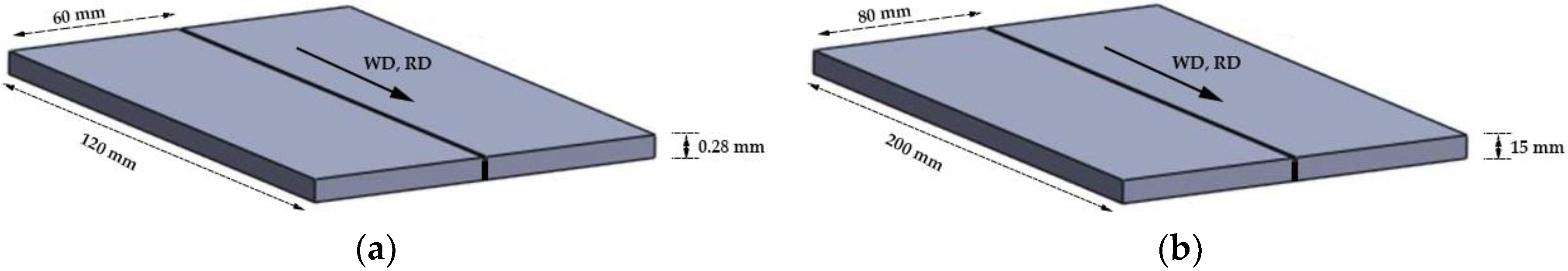
A single pass square butt joint automated weld was made along the rolling direction (RD) of the rolled sheets, using the GTAW process (Figure 1) according to AWS C5.5 [26]. Argon, at a flow rate of 10 L/min, was used as a shielding gas. The welding parameters for the weld joints are given below in Table 3.
For the results shown here, we first obtain the MASC curve for each steel grade, in the laboratory. The methodology for obtaining these MASC curves is the following: Each sample of ferromagnetic steel, similar to the base materials of the welds, is subjected to successive stresses levels, both tensile and compressive, in the elastic deformation range of the material and below the Villari point, to ensure that only residual stresses are induced. The stresses may be induced in a controlled manner using a device that allows the control of the level of stress, via a load cell, and its rate of change, e.g., an INSTRON machine (300DX type) (Analytical Instruments SA, Athens, Greece). At each stress level, the sample is unloaded and is measured. Its peak value, , is plotted against the applied stress level [23].
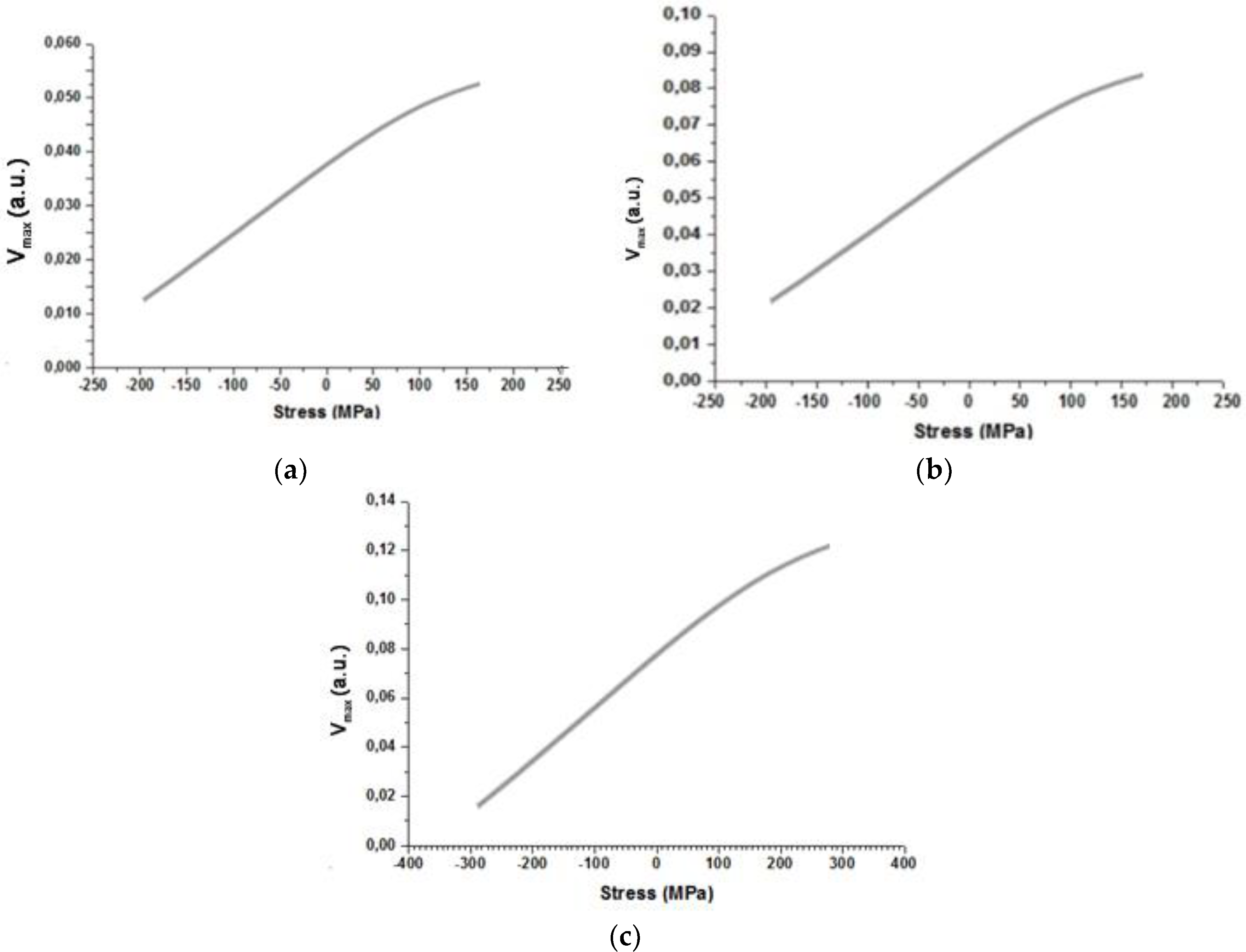
The magnetic parameter, , is measured using ac magnetometry (NTUA in-house instrument, Athens, Greece), along the rolling direction, of the unloaded pre-strained samples. A programmable function generator connected to a power amplifier generates the low frequency (0.5 Hz) sinusoidal current fed to the excitation coil of a yoke-shaped sensor forming a closed magnetic circuit with the sample. The sample is magnetized by the excitation field, , and the resulting time-varying magnetization induces a sinusoidal output voltage , at the ends of a sensing coil, according to Faradays’ law. It is easily shown that is proportional to . If the material is enclosed by the sensing coil, we measure the bulk permeability; if it is perpendicular to it, we measure the surface permeability. Here we report on bulk permeability measurements. The value we record is the peak value of the output voltage, , which is proportional to , and which occurs at a field close to the coercivity of the material. Because the sensor is not calibrated against a standard steel sample, we report the measured values and not values. The proportionality constant between and can be roughly estimated from the excitation field and sensing coil parameters resulting in the following approximate values: 56, 1.5 and 1.7 mWb/Am, for NOES, AISI1008 and AISI4130 respectively. Each measurement is repeated six times. Plotting vs. we obtain the MASC curve of a given material (Figure 2). The MASC curves shown in Figure 2 correspond to bulk permeability measurements.
Once the MASC curve for each steel grade is determined, we proceed with the measurement of permeability on the welded samples. It is important that the same sensor is used for these measurements, as well. The measurements have been carried out at regular intervals of 0.5 mm parallel and perpendicular to the weld direction starting from 15 mm away from the weld edges at each side of the weld specimen to include all three welding regions, namely the BM, the HAZ and the FZ, and to avoid edge effects due to cutting [23]. Then, using the permeability measurements and the corresponding MASC curve we can determine the residual stress levels at each point of measurement.
To investigate the effectiveness and efficiency of our method, we compared the residual stress profiles thus obtained against diffraction measurements. XRD is used in the Bragg–Brentano set-up (XRD-BB) in order to determine the average of local surface microstrains in the area of measurement, which are correlated with surface permeability measurements. ND measurements provide the reference measurements for bulk permeability. The uncertainty of XRD-BB can be brought down to 1–5% [27] by appropriate control of the photonic excitation as well as optimization of the counts averaging method. Similar techniques have been applied for the ND measurements shown here. XRD measurements were carried out using Cr-Kα radiation X-ray tube, operating with a target current of 5 mA at 30 kV. ND measurements were carried out at the Nuclear Station Rez near Prague (Nuclear Station Rez near Prague, Rez, Czech Republic), with an accuracy of 5%, along the (110) crystallographic plane of the ferrite. The experimental procedure is discussed in detail in [23,24,25]. The corresponding residual stresses are calculated using Young’s modulus and Poisson’s ratio of each steel grade. Young’s moduli, , have been determined from the gradient of the linear portion (elastic region) of the stress-strain curves. They have been found to be 210 GPa, 225.5 GPa, and 225 GPa for NOES, AISI 1008 and AISI 4130 respectively; the Poisson’s ratio, , was taken equal to 0.28.
Finally, microstructural characterization using SEM is carried out in order to investigate changes in microstructure in all three welding zones: BM, HAZ, FZ. Metallographic samples were extracted from the welded plates and polished with 800 to 2400 grit SiC paper followed by 3 μm and 1 μm diamond paste suspension to obtain mirror finish, and etching using 2% Nital solution.
3. Results
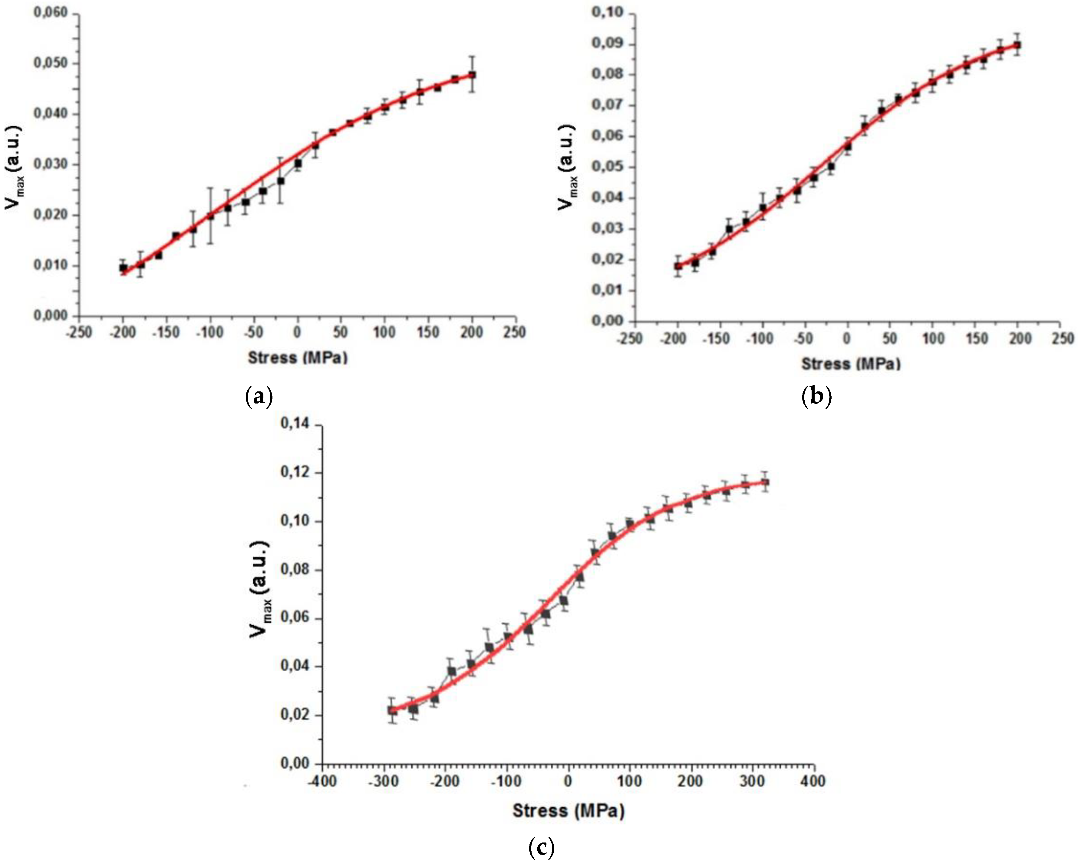
Figure 2 illustrates the bulk MASC curves for the three steel grades examined. Compressive (negative) and tensile (positive) residual stress values in MPa are plotted on the horizontal axis. The sensor’s peak output voltage, , corresponding to measured at each given stress level, is plotted on the vertical axis (in arbitrary units because the sensor is uncalibrated.)
All three curves follow a similar sigmoidal trend. increases with tensile and decreases with compressive stress. Since all three steels have positive magnetostriction, the results are in line with the Le Chatelier equilibrium principle: the magnetization along the stress direction increases, if the signs of magnetostriction and applied stress are the same, and vice versa. No hysteretic effects have been observed and this contributes to a lower uncertainty of the measurement [23,24,25].
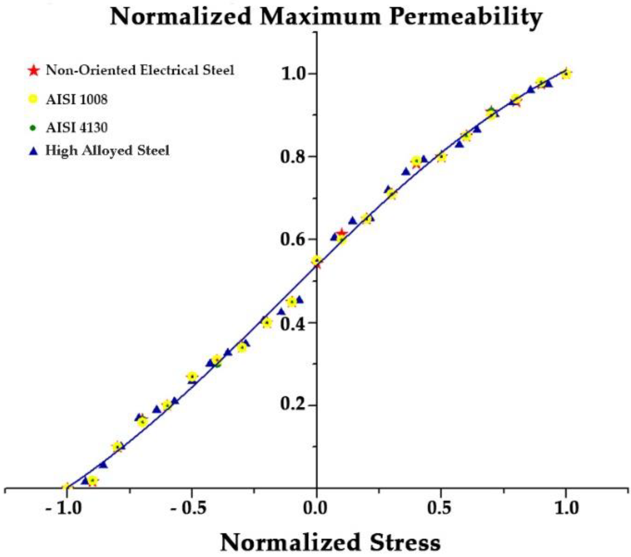
Τhe curves were normalized using yield stress, σY, as a proxy. The yield stress values used were 200 ΜPa for NOES, 214 ΜPa for AISI 1008 and 280 ΜPa for AISI 4130.
The use of a normalized curve greatly facilitates the determination of the residual stress value at the under-examination region of each welding sample. It simplifies the mapping of the stress profile as it allows the evaluation of residual stresses with respect to the fractional deviation from the unstressed state (zero point).
To determine the normalized magnetic permeability and stress values, and respectively, the following formulas are used:
where (, ) is the th point on the MASC curve, (, ) is the point corresponding to the maximum tensile stress point, and (, ) is the point corresponding to the maximum compressive stress point (Figure 2).
Figure 3 shows the normalized calibration curves of the three aforementioned steel grades as well as the MASC curve of a high alloyed steel. All normalized curves seem to collapse into one which suggests the existence of a universal curve.
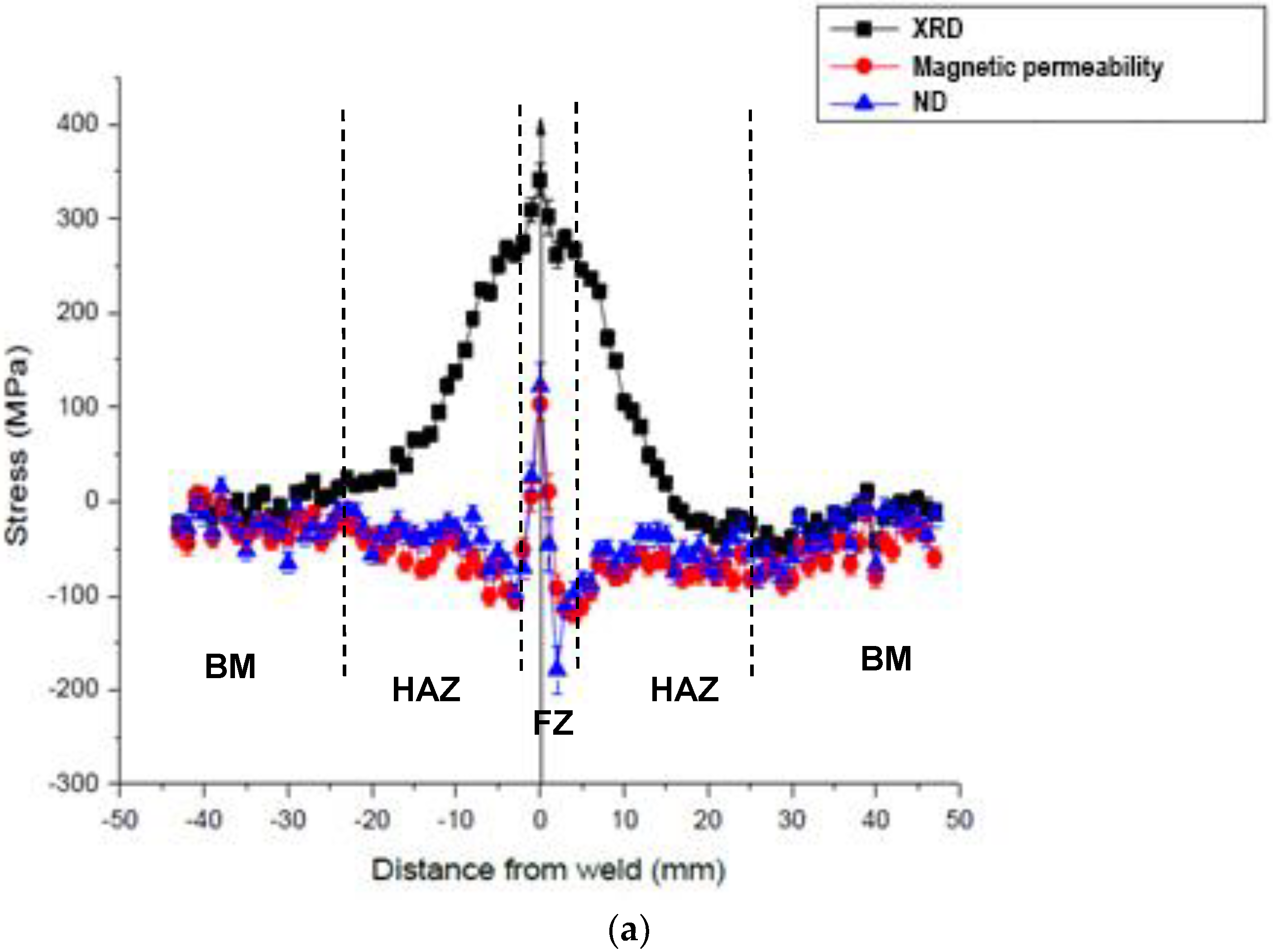
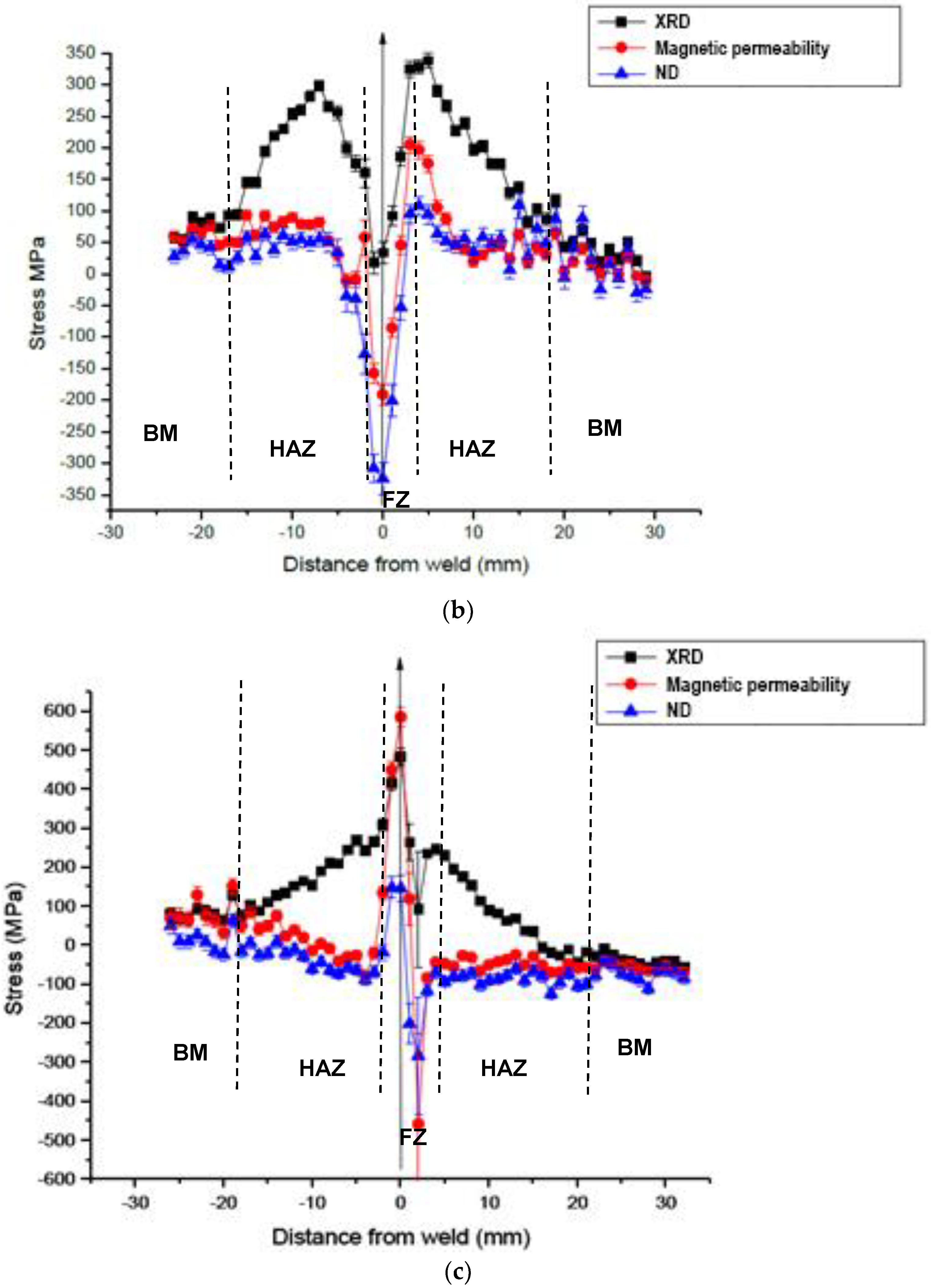
Figure 4 presents the distribution of residual stress values on either side of the FZ centerline, as determined via XRD, ND, and bulk magnetic permeability measurements for all three types of steel. The permeability values shown correspond to measurements across the weld, in the middle of each sample; i.e., at 60 mm from the edge for the NOES sample and at 100 mm form the edge for the other two steel grades.
As already mentioned, MASC curves are obtained for the elastic region only. To determine stresses outside the MASC curve range, extrapolation is used. The extent of the validity of this approach is currently under study.
The profiles of the residual stresses measured using diffraction techniques exhibit similar trends as well as differences, which are attributed to the difference in volume of inspection and penetration depth in each case. The XRD measurements are sensitive to surface conditions with an assumed penetration depth in the order of 20 μm, while for the ND measurements, the residual stress value is the average over an effective penetration depth of 5 mm. For NOES and AISI 4130 samples (Figure 4a,c), XRD measurements reveal a tensile bell-shaped stress profile that increases sharply around the weld line and tends to zero exponentially moving away from the weld line. ND measurements show high tensile and compressive stresses in the FZ and compressive stresses in the HAZ, which tend to zero away from the weld line. In the case of AISI 1008 (Figure 4b), the bell-shape profile was inversed possibly due to the difference in the heat dissipation profile in this steel grade, as a result of the welding procedure. In all cases, stress, tensile or compressive, gradually tends to zero as the BM region is approached.
With known and , Equations (1) and (2) have been used to determine residual stress values , from permeability measurements and the normalized curve of Figure 3. The stress profiles thus obtained are similar to the ND curves. This is strong evidence for the validity of our method since the MASC curves used for the stress profile determination were based on bulk permeability measurements. Significant deviations are observed near the centerline where the microstructural changes due to welding are dramatic. FZ is of higher complexity than the other two regions and requires further study.
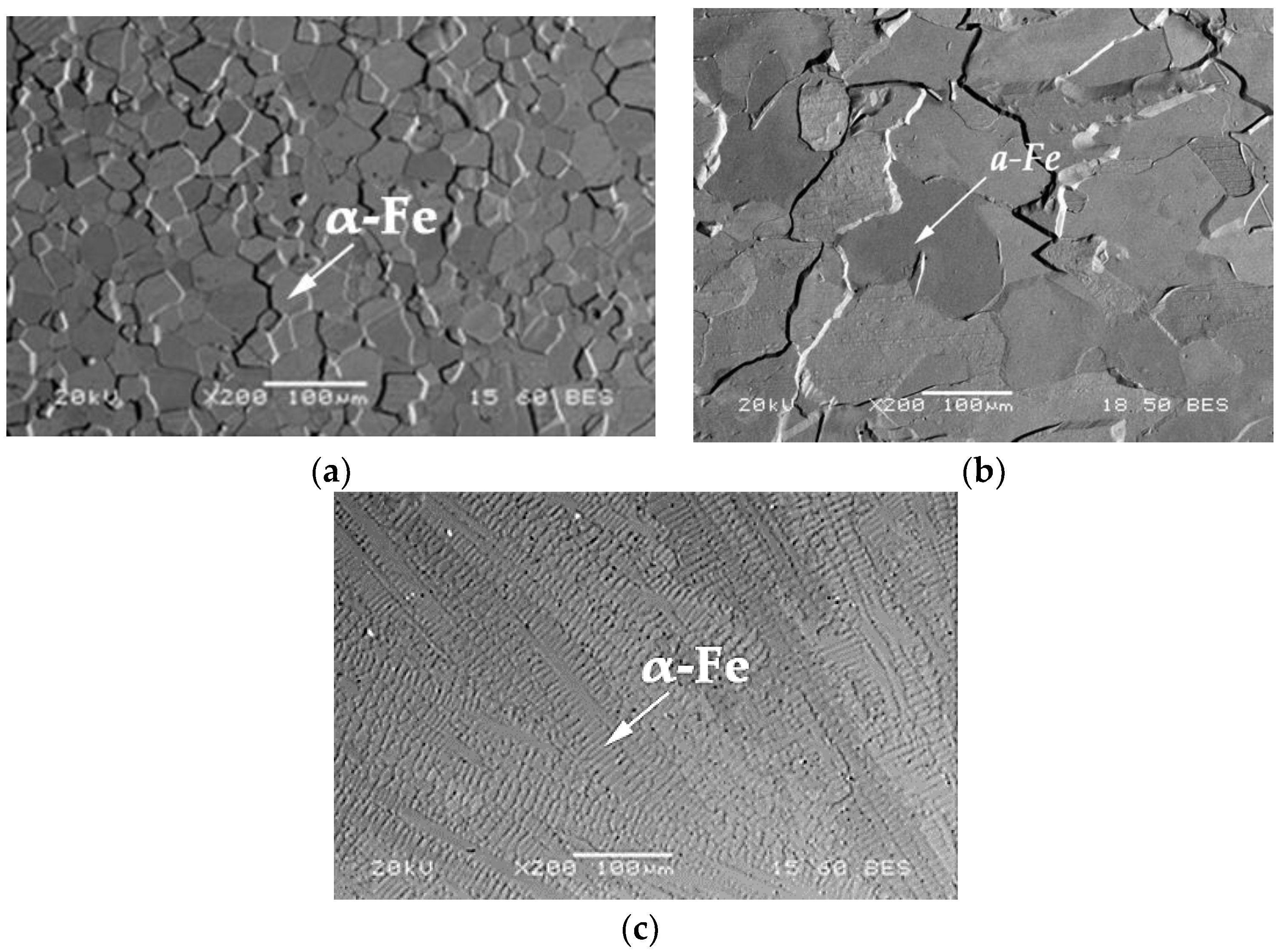
The microstructural studies of the base metal and welded joints samples were performed using SEM on the above welded samples. The metallographic evaluation showed that the BM of the NOES welded sample consisted of a single-phase ferrite matrix (Figure 5a). Figure 5b illustrates the microstructure in the heat affected zone which consists of an almost completely recrystallized elongated ferrite structure with a quite homogeneous grain size distribution, which is in line with the lower stresses measured there. Dendrite groups of α-ferrite developed in the FZ (Figure 5c) during the solidification process, which make the microstructure highly inhomogeneous. The stress profile in that region is quite complex as is the microstructure and tests the limits of our method.
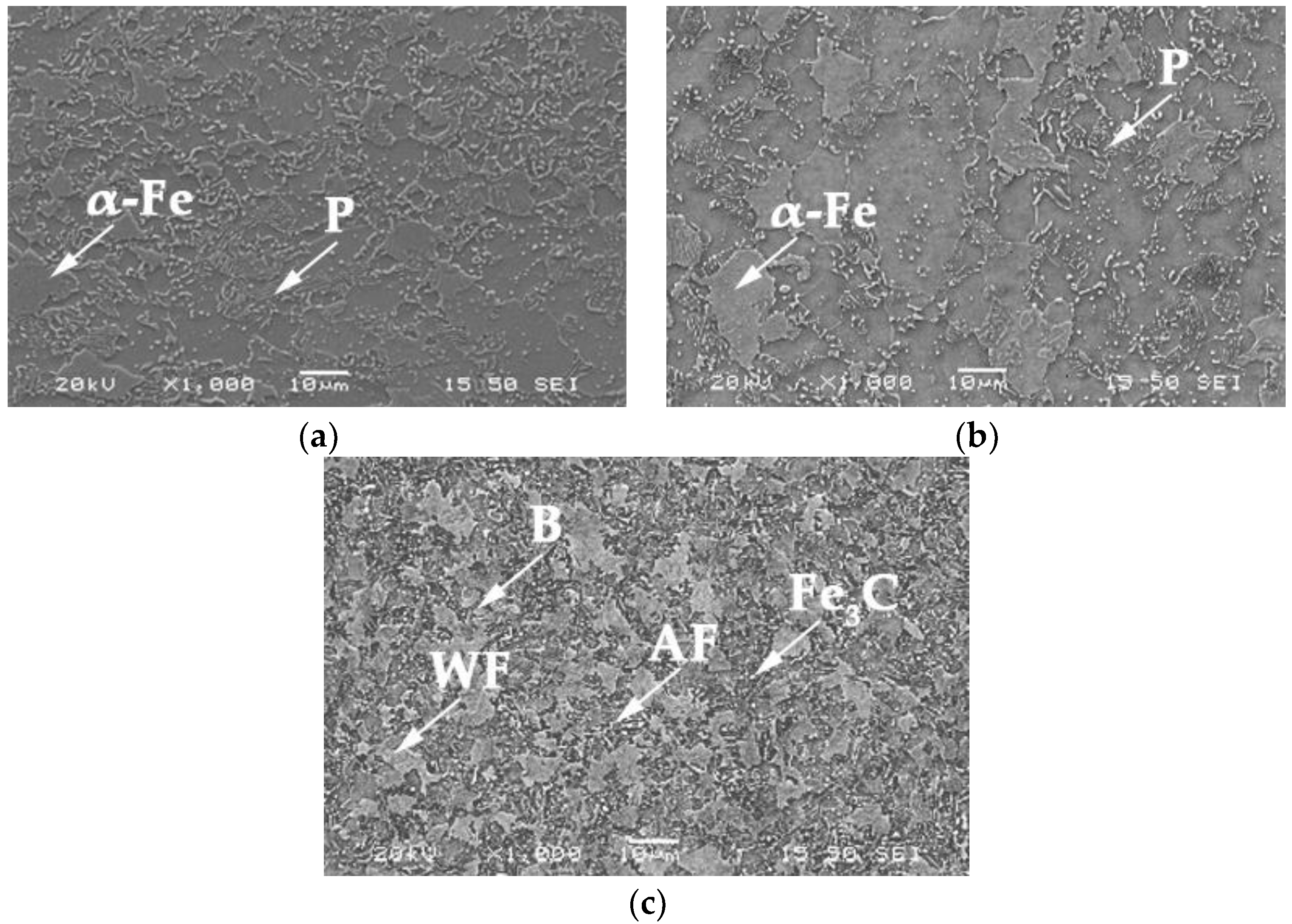
The BM of the AISI 1008 welded sample has shown predominantly equiaxed proeutectoid ferrite grains (α-Fe) and low volume fraction of banded-structured pearlite (P) (Figure 6a). The HAZ microstructure comprised finer pearlite and uniformly distributed carbides in polygonal ferrite grains (Figure 6b). On the other hand, the FZ is comprised of acicular ferrite (AF) and Widmanstätten ferrite (WF) as parallel ferrite laths, thermodynamically unstable bainite (B) and cementite (Fe3C) (Figure 6c).
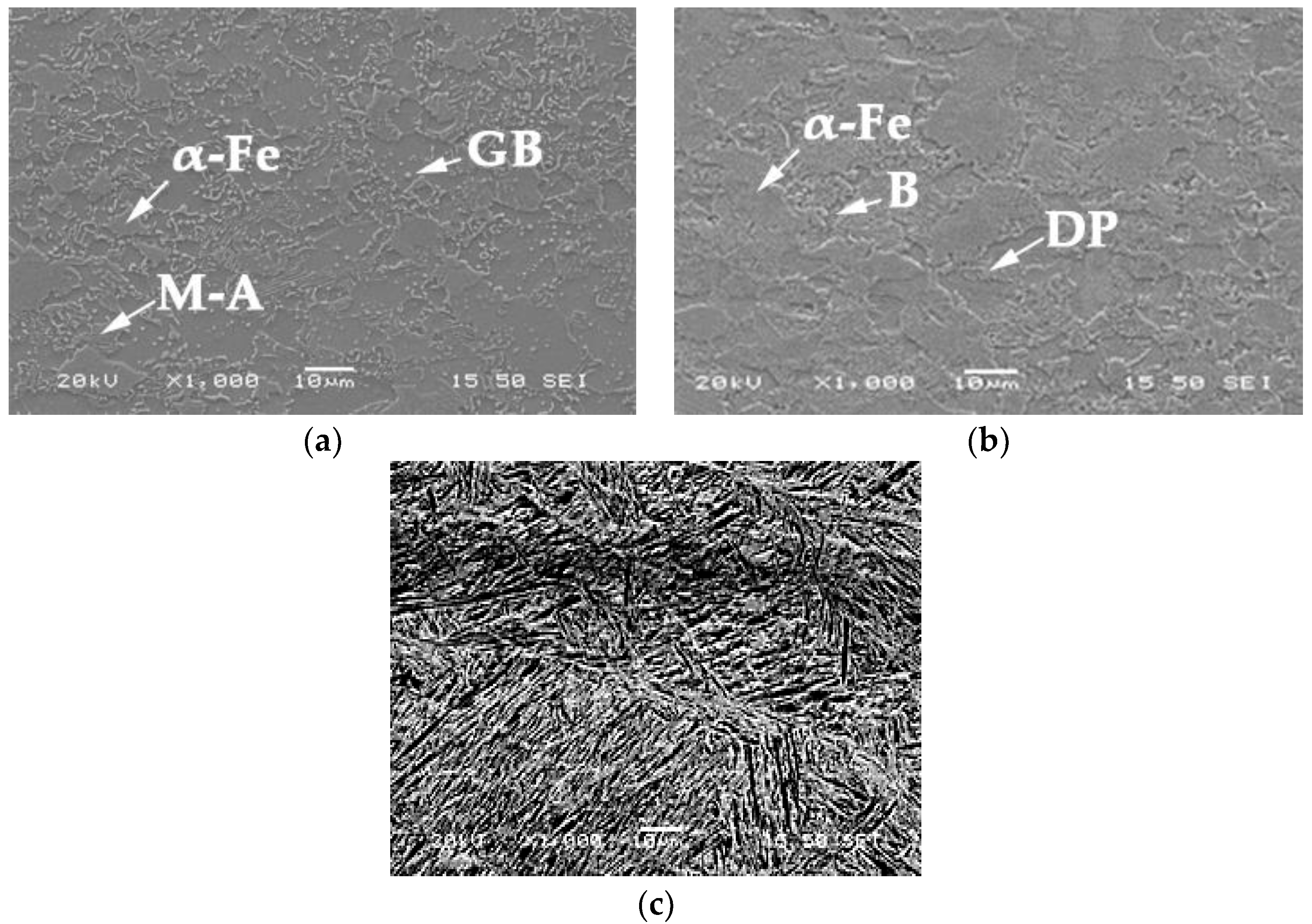
Figure 7 illustrates the microstructural complexity developed at the weld joints of AISI 4130 welded sample. The microstructure of the BM consists mainly of ferrite grains (α-Fe) with regions of martensite-austenite (MA) constitutes and presumably granular bainite (GB) (Figure 7a). The martensite is characterized by an absence of carbide precipitation, whereas an extensive carbide precipitation was observed on the bainitic structure. The diverse constituents of the multiphase HAZ are shown in Figure 7b. A continuous network of polygonal ferrite grains is observed with the remaining part of the structure consisting of degenerated pearlite (DP), acicular platelets of bainite (B) arranged in the form of islands within a ferrite matrix. A full martensitic structure is the dominant microstructure of the FZ as illustrated in Figure 7c.
4. Discussion
The magnetic non-destructive method presented consists of two phases: (a) the preparation phase where we obtain the calibration curves for the ferromagnetic material to be studied; (b) the evaluation phase where the residual stresses are determined using the aforementioned calibration curves.
4.1. Magnetic Measurements
In this work, we focus on the comparison of our method with standardized methods, such as diffractometry, for determining residual stresses. More specifically, in order to evaluate the accuracy and the limitations of our method, we focus on the comparison between the MASC curves obtained in the laboratory (Figure 2) and the permeability vs. strain dependence (Figure 8 and Figure 9) as inferred from the diffraction and permeability measurements across welds which are depicted on Figure 4.
At the atomic level, under the influence of an externally applied magnetic field, the spins of a ferromagnetic substance, ordered in domains of various directions, rotate reversibly or irreversibly towards the applied field in order to minimize their internal energy, which increases due to the external stimulus. In this process, called the magnetization process, the rotation is affected or even hindered by lattice deformation, voids, inclusions, or other irregularities in the crystal structure. In an analogous manner, at the microscopic level, the magnetic domains rotate, expand, or collapse via the movement of domain walls. The domain wall movement is affected or hindered by the size of grains, the grain boundaries, and the different phases in the material. The amount of energy required to overcome these barriers and manage the alignment of the spins or domains with the field is reflected in the hysteresis loop of a material.
The residual stresses are the result of lattice strains, which may be also evident at the grain level. These strains are, therefore, expected to affect the magnetization process. This is reflected on the macroscopic measurement of the hysteresis loop, . Therefore, the loop, and its derivative, , links the macroscopic measurement to the strain affected microstructure.
The parameter we have chosen to record, the maximum differential permeability, , is an indication of the propensity of the material to align with the magnetic field. The process is assisted by stress fields along the direction of the measurement and hindered by fields at an angle to it. In positive magnetostrictive materials, such as the ones examined in this work, this means that the material’s magnetization tends to rotate easier towards the applied field as the tensile stress increases, which results in higher permeability values. This is why the MASC curves of Figure 2 show that permeability increases with tensile stress and decreases with compressive stress. In other words, the residual stress field acts as an effective anisotropy field, in the absence of external loading. From the point of view of continuum mechanics, the presence of an effective stress field, residual or applied, increases the internal energy of the material. In order for the material to accommodate this additional energy, it reconfigures its microstructure and this is reflected on the macroscopic magnetic behavior.
During the measurement of a MASC curve, such as those of Figure 2, known tensile and compressive stresses are applied along the rolling direction of the sample. For each stress level, the underlying microstructure reconfigures to accommodate the additional energy. After the removal of the given load, this reconfiguration leads to residual strain, which is reflected on the magnetic parameter measured. Note that, in this case, the accuracy of this applied stress depends on the accuracy of the load cell controlling the applied load and the accuracy of the magnetic parameter measurement depends on the accuracy of the permeability sensor used.
The MASC curve of Figure 2, shows that all curves are sigmoidal, which is characteristic of magnetization processes. NOES and AISI 1008 have similar yield stress but NOES has significantly lower permeability which may be related to the fact that it is non-oriented. AISI 4130 has the highest permeability of the three and the highest yield stress.
These MASC curves correspond to samples of the BM of the welds. And yet, we use them to determine residual stresses in welds which result from thermal processes and phase transformations.
We postulate that the macroscopic magnetic parameter , which is recorded, depends on the aggregate effect of the underlying microstructure and does not distinguish between the origins or the causes of this microstructure. The permeability, as a function of residual stress, does not depend on the way the stress is induced; i.e., via an INSTRON machine in the laboratory or via thermal processing as in welding. The basis of our analysis is that the local residual microstrains are the result of added energy either in the form of applied stress or heat. In either case, the grains have realigned, expanded or shrank to accommodate the added energy without entering the plastic deformation region. In either case, the magnetic parameter will yield the same value for the same effective residual stress field.
By using the universal MASC curve of Figure 3 to determine the residual stresses across the weld shown in Figure 4, we operate on the assumption that mainly residual stresses are present in all three zones. This may be true for the HAZ and the BM but it tests the limits of our method in the case of the FZ where there is a phase transformation and most likely the material has entered in the plastic deformation region. This is corroborated by the experimental evidence (Figure 4), which shows good quantitative agreement between ND and permeability measurements in the HAZ and the BM and significant deviations in the FZ, even though the general trends are preserved.
4.2. Microstructural Studies
From a metallographic point of view, the NOES sample has a single-phase ferrite matrix which along with the low degree of anisotropy is responsible for the softer magnetic response and low permeability values measured. The AISI 4130 sample, on the other hand, revealed a packet martensite structure, which contains several bundles of laths. Small amounts of retained austenite were detected as inter-lath films while no carbide precipitation was observed on granular bainite (Figure 7a) [27]. Higher maximum permeability values along the rolling direction are in line with the stronger anisotropy of this steel grade, which is enhanced with tensile stresses, due to positive magnetostriction.
Finally, the combination of pearlite and ferrite in the AISI 1008 sample yield several magnetic phases as well with a variable profile of local anisotropies. This results in lower permeability values than in AISI 4130 and higher than NOES. AISI 1008 presents a slight asymmetry between the tensile and compressive stress range, which may be due to a non-negligible Bauschinger effect and needs to be further investigated [9,10,11].
The microstructural differences between the examined welded samples are illustrated in Figure 5, Figure 6 and Figure 7. In the NOES welded sample, the equiaxial ferrite of the base material, became polygonal and heterogeneously distributed in the HAZ and transformed to metastable ferrite dendrite groups in the weld metal. It is evident that no phase transformation occurred during the solidification. Only the morphology and the grain size of ferrite grains has been changed. The metastable dendrite structure is compatible with higher anisotropy along the weld which may explain the sharp increase in the permeability observed around the FZ (Figure 4a). The larger grains in the HAZ, with no phase transformation, suggest that the heat dissipated during the welding has been accommodated by the ferrite grains of the BM by enlarging their size and favoring compressive stresses (Figure 4b).
For AISI 4130 weld metal, the SEM images (Figure 7) show an arc welded joint with martensitic structure. Martensitic transformation is displacive and accommodated with significant increase in specific volume. The latter counters the volume contraction due to the shrinkage of weld metal, releasing the measured tensile residual stresses (Figure 4c). Hence, the martensite transformation contributes towards the development of residual stresses. The diverse constituents of the BM (ferrite grains, martensite-austenite constitutes and granular bainite) were transformed to ferrite grains, degenerated pearlite and acicular bainite in the HAZ. Thus, reconstructive as well as displacive transformations occurred during solidification in the HAZ. The formation of pearlite and bainite in the HAZ occurred at high temperature and did not contribute much towards the development of residual stresses [28,29,30]. The tensile stresses in the FZ were counterbalanced by the compressive ones in the HAZ. The enrichment of ferrite with carbon within the supersaturated solid solution of martensite is related to an increase in the magnetic permeability [28,29,30]. In the HAZ, the elongation of the ferrite grains and the presence of low defect microstructures lead to intermediate values of permeability. Additionally, the formation of no layer structured degenerated pearlite is associated with the scarce carbon diffusion, which is promoting the classical pearlite lamellae structure. Thus, the compressive stresses in the HAZ (Figure 4c) favor the lower permeability values and may be related to the curved morphology of pearlite.
The metallographic evaluation of the AISI 1008 welded sample revealed the transformation of ferrite and pearlite to acicular ferrite, Widmanstätten ferrite, bainite, and cementite (Figure 6). The M-shape profile for residual stress may be attributed to the phase transformation of ferrite—pearlite initially in the BM material to grain boundary ferrite, acicular ferrite, Widmanstätten ferrite, bainite, and micro alloying phase. In the microstructure of FZ, the eutectic metastable M2C or the stable M6C phase carbides forms may also be detected. Although, tensile stresses were expected to be found in the FZ, compressive stresses are detected instead, possibly due to the presence of a high percentage of displacively transformed ferrite phases (Figure 4b). From the inversed-bell stress profile, it is observed that the stress values are gradually increased while moving from the FZ to the unaffected BM. The —shape residual stress profile also indicate that the dimensions of the sample, as well as the parameters of the welding procedure were not the optimal ones.
4.3. Validation of Results
In order to test the validity of our assumptions, we plotted the magnetic permeability values measured across the welds in the three samples against the stress values determined by diffraction methods at the respective points. Points with stress measurements lying outside the elastic region have been excluded. The results are shown on Figure 8. The curves thus obtained are consistent with the MASC curves obtained in the lab (Figure 2).
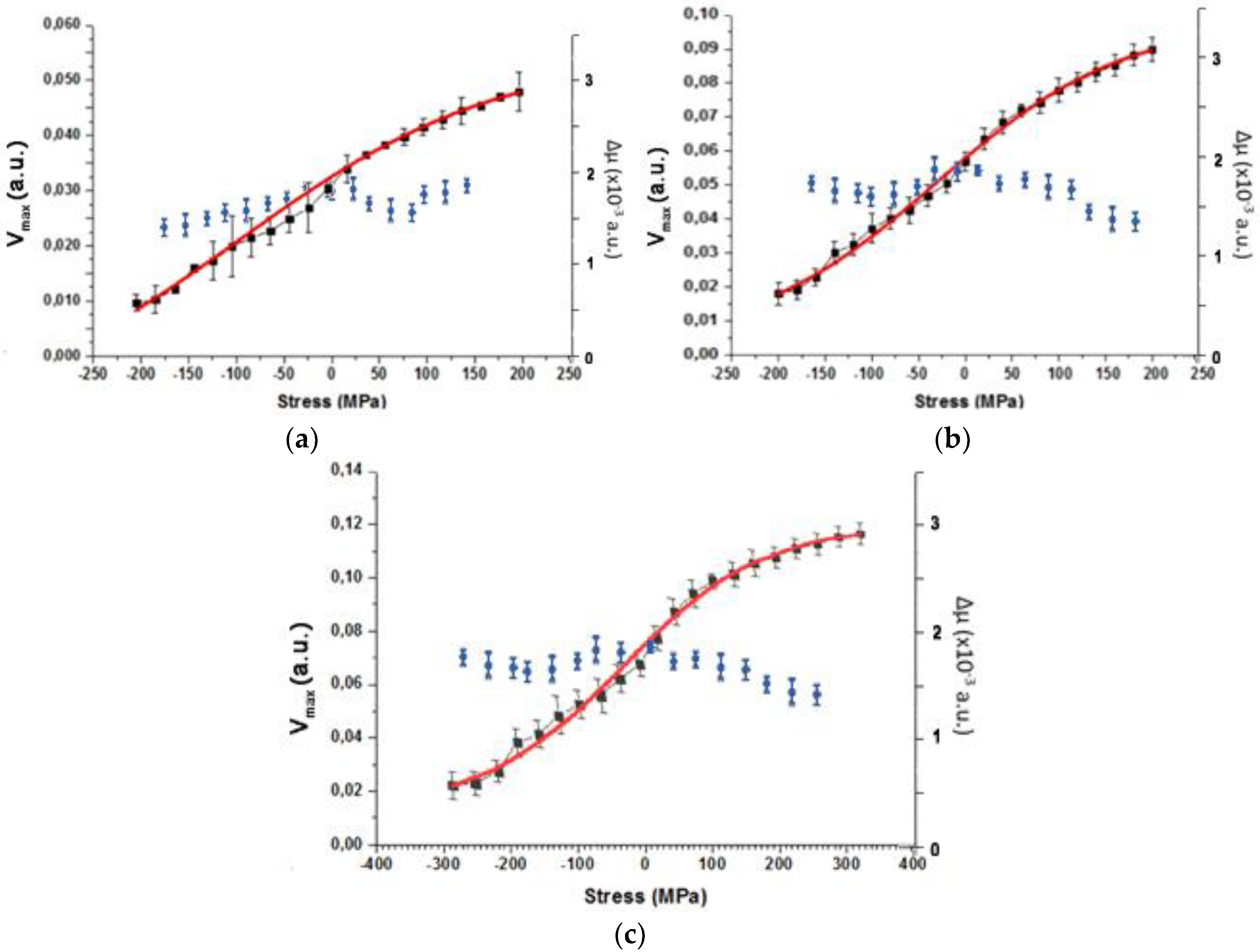
Next, in order to evaluate the uncertainty level of our measurements, we calculated the difference, , between the permeability values measured on unwelded samples in the laboratory for the MASC curves and the permeability values measured on welded samples for comparable levels of residual stress, as measured by ND. Figure 9 compares the curve of vs. stress for each sample (blue marks) against the MASC curves of Figure 2. The uncertainty level, in all cases, is very low and between 0.1% and 0.2%. It should be noted that the magnetic measurements have been carried out manually, which partly contributes to the uncertainty. Further studies are necessary to establish the sources of uncertainty and their correlation with respective residual stress levels.
Overall, the proposed magnetic non-destructive method yields reliable results when compared with standardized methods, such as ND. Contrary to the latter, the magnetic method does not require specialized facilities and highly trained personnel. It is applicable in both the laboratory and the field, it is fast and it is cost effective. Once a calibration curve has been obtained for a specific grade of steel, a portable sensor with built-in post processing software suffices to carry out the permeability measurement and convert it to residual stress. When applying the proposed magnetic method for residual stress evaluation, it is important that the following are ensured: (a) the operating conditions in the measurement setup used for the calibration curves are the same throughout the measurement (b) the same sensor is used for the MASC curve and the determination of the stresses in the welds.
The speed of measurement is limited only by the frequency of the excitation field and the speed of the post processing algorithm. In our new pending-for-patent surface permeability sensors the speed of measurement can be as high as 10 μs per point of measurement, while with our yoke-type permeability sensors, used in this work, the speed of measurement is limited to a few ms per point.
The new magnetic method is also superior with respect to the uncertainty of the measurement. The reference stress measurements obtained by XRD-BB of ND have an uncertainty of 1–5% [31,32,33,34,35,36,37], in the best case. The accuracy of the proposed method depends on the uncertainty of the stress measurements of the MASC curves as well as on the uncertainty of the permeability sensor. Using a load cell-controlled stress-strain instrument for the MASC curves, the uncertainty of the stress measurements depends on the uncertainty of the load cell or other strain sensor used, which typically is in the range of 0.1% or less. On the other hand, our permeability sensors have a maximum uncertainty of 0.01%, after temperature and displacement correction.
5. Conclusions
The presented method is a tool for the quantitative assessment of the residual stress fields in steels along the direction of the magnetic measurement. It takes advantage of the link between microstructure and magnetic phenomenology and uses the maximum value of the differential permeability as a metric. It provides a roadmap to obtaining the MASC curve for the under-test material, which is the permeability vs. residual stress characteristic. Using the MASC curve as a calibration curve, the residual stresses in a material can be determined with a simple permeability measurement, regardless of the origin of the residual stress. The method can be applied in the laboratory or the field with accuracy better than 1% and speed that can be as high as 10 μs per point of measurement, depending on the mechanical devices used to obtain the MASC curve and the sensors used for the magnetic measurements.
In this work, we presented the application of the method in GTAW welds of three different steel grades. The results obtained with the new method are in very good quantitative agreement with those obtained with diffractometry, especially in the heat affected zone and the base metal, where elastic residual stresses are predominant. The applicability of the method for the fusion zone, where phase transformations and plastic deformation are expected, needs to be further investigated. Another important question of further research is the existence of universality underlying the calibration curves, which is likely to enhance our knowledge on magnetomechanical coupling and thus achieve better control of the process.
Author Contributions
Conceptualization, E.H.; Methodology, E.H. and P.V.; Software, P.V.; Validation, A.K. and P.T.; Formal Analysis, P.V. and A.K.; Data Curation, P.V.; Investigation, P.V.; Writing-Original Draft Preparation, P.V.; Writing-Review & Editing, A.K., P.T. and E.H.; Visualization, P.V.; Supervision, E.H.; Project Administration, E.H.
Acknowledgments
Acknowledgements are due to the researchers of the nuclear station Rez near Prague and Peter Svec, Slovak Academy of Sciences.
Conflicts of Interest
The authors declare no conflict of interest.
References
- Withers, P.J.; Bhadeshia, H.K.D.H. Residual stress Part 1—Measurement techniques. Mater. Sci. Technol. 2001, 17, 355–365. [Google Scholar] [CrossRef]
- Nasir, N.S.M.; Razab, M.K.A.; Mamat, A.S.; Ahmad, M.I. Review on welding residual stresses. ARPN J. Eng. Appl. Sci. 2016, 11, 6166–6175. [Google Scholar]
- Withers, P.J.; Bhadeshia, H.K.D.H. Residual stress Part 2—Nature and origins. Mater. Sci. Technol. 2001, 17, 366–375. [Google Scholar] [CrossRef]
- Lu, J.; Retraint, D. A review of recent development and applications in the field of X-ray diffraction for residual stress studies. J. Strain Anal. 1998, 33, 127–136. [Google Scholar] [CrossRef]
- Park, M.J.; Yang, H.N.; Jang, D.Y.; Kim, J.S.; Jin, T.E. Residual stress measurement on welded specimen by neutron diffraction. Mater. Sci. Technol. 2004, 83, 381–387. [Google Scholar] [CrossRef]
- Liu, M.; Kim, J.Y.; Qu, J.; Jacobsa, L.J. Measuring Residual Stresses using nonlinear ultrasounds. AIP Conf. Proc. 2010, 1211, 1365–1372. [Google Scholar]
- Prevéy, P.S. Χ-ray Diffraction Residual Stress Technique; Lambda Research, Inc.: Littleton, MA, USA, 1986; Volume 4. [Google Scholar]
- Jiles, D.C. Review of magnetic methods for nondestructive evaluation. NDT E Int. 1988, 21, 311–319. [Google Scholar] [CrossRef]
- Takahashi, S.; Kobayashi, S.; Kikuchi, H.; Kamada, Y. Relationship between mechanical and magnetic properties in cold rolled low carbon steel. J. Appl. Phys. 2006, 100, 113908. [Google Scholar] [CrossRef] [Green Version]
- Takahashi, S.; Kobayashi, S.; Tomáš, I.; Dupre, L.; Vértesy, G. Comparison of magnetic nondestructive methods applied for inspection of steel degradation. NDT E Int. 2017, 91, 54–60. [Google Scholar] [CrossRef] [Green Version]
- Kobayashi, S.; Takahashi, H.; Kamada, Y. Evaluation of case depth in induction-hardened steels: Magnetic hysteresis measurements and hardness-depth profiling by differential permeability analysis. J. Magn. Magn. Mater. 2013, 343, 112–118. [Google Scholar] [CrossRef]
- Jarvis, R.; Cawley, P.; Nagy, P.B. Performance evaluation of a magnetic field measurement NDE technique using a model assisted Probability of Detection framework. NDT E Int. 2017, 91, 61–70. [Google Scholar] [CrossRef]
- Gomes, E.; Schneider, J.; Verbeken, K.; Barros, J.; Houbaert, Y. Correlation between microstructure, texture, and magnetic induction in nonoriented electrical steels. IEEE Trans. Magn. 2010, 46, 310–313. [Google Scholar] [CrossRef] [Green Version]
- De Campos, M.F.; Sablik, M.J.; Landgraf, F.J.G.; Hirsch, T.K.; Machado, R.; Magnabosco, R.; Gutierrez, C.J.; Bandyopadhyay, A. Effect of rolling on the residual stresses and magnetic properties of a 0.5% Si electrical steel. J. Magn. Magn. Mater. 2008, 320, e377–e380. [Google Scholar] [CrossRef]
- Augustyniak, B.; Chmielewski, M.; Piotrowski, L.; Kowalewski, Z. Comparison of Properties of Magnetoacoustic Emission and Mechanical Barkhausen Effects for P91 Steel after Plastic Flow and Creep. IEEE Trans. Magn. 2008, 44, 3273–3276. [Google Scholar] [CrossRef]
- Stupakov, O.; Uchimoto, T.; Takagi, T. Magnetic anisotropy of plastically deformed low-carbon steel. J. Phys. D Appl. Phys. 2010, 43, 195003. [Google Scholar] [CrossRef] [Green Version]
- Stupakov, O. Local Non-contact Evaluation of the ac Magnetic Hysteresis Parameters of Electrical Steels by the Barkhausen Noise Technique. NDT E Int. 2013, 32, 405–412. [Google Scholar] [CrossRef]
- O’Sullivan, D.; Cotterell, M.; Tanner, D.A.; Meszaros, I. Characterisation of ferritic stainless steel by Barkhausen techniques. NDT E Int. 2004, 37, 489–496. [Google Scholar] [CrossRef]
- Anglada-Rivera, J.; Padovese, L.R.; Capó-Sánchez, J. Magnetic Barkhausen Noise and hysteresis loop in commercial carbon steel: Influence of applied tensile stress and grain size. J. Magn. Magn. Mater. 2001, 231, 299–306. [Google Scholar] [CrossRef]
- Buttle, D.J.; Briggs, G.A.D.; Jakubovics, J.P.; Little, E.A.; Scruby, E.A. Magnetoacoustic and Barkhausen emission in ferromagnetic materials. Philos. Trans. A Math. Phys. Eng. Sci. 1986, A320, 363–376. [Google Scholar] [CrossRef]
- Dubov, A.; Kolokolnikov, S. Assessment of the Material State of Oil and Gas Pipelines Based on the Metal Magnetic Memory Method. Weld. World 2012, 56, 11–19. [Google Scholar] [CrossRef]
- Tomáš, I.; Kadlecová, J.; Vértesy, G. Measurement of Flat Samples with Rough Surfaces by Magnetic Adaptive Testing. IEEE Trans. Magn. 2012, 48, 1441–1444. [Google Scholar] [CrossRef]
- Hristoforou, E.; Vourna, P.; Ktena, A.; Svec, P. On the Universality of the Dependence of Magnetic Parameters on Residual Stresses in Steels. IEEE Trans. Magn. 2016, 52, 6201106. [Google Scholar] [CrossRef]
- Vourna, P.; Hervoches, C.; Vrána, M.; Ktena, A.; Hristoforou, E. Correlation of Magnetic Properties and Residual Stress Distribution Monitored by X-ray & Neutron Diffraction in Welded AISI 1008 Steel Sheets. IEEE Trans. Magn. 2015, 51, 6200104. [Google Scholar] [CrossRef]
- Vourna, P.; Ktena, A.; Tsakiridis, P.E.; Hristoforou, E. A novel approach of accurately evaluating residual stress and microstructure of welded electrical steels. NDT E Int. 2015, 71, 33–42. [Google Scholar] [CrossRef]
- American Welding Society. AWS C5.5/C5.5M: An American National Standard, Recommended Practices for Gas Tungsten Arc Welding; AWS: Miami, FL, USA, 2003. [Google Scholar]
- Fielding, L.C.D. The Bainite Controversy, Materials Science and Technology. Mater. Sci. Technol. 2013, 29, 383–399. [Google Scholar] [CrossRef]
- Jiles, D.C.; Verhoeven, J.D. Investigation of the Microstructural Dependence of the Magnetic Properties of 4130 Alloy Steels and Carbon Steels for NDE; Springer: Boston, MA, USA, 1987; pp. 1681–1690. [Google Scholar]
- Solano-Alvarez, W.; Abreu, H.F.G.; da Silva, M.R.; Peet, M.J. Phase quantification in nanobainite via magnetic measurements and X-ray diffraction. J. Magn. Magn. Mater. 2015, 378, 200–205. [Google Scholar] [CrossRef]
- Zhou, L.; Liu, J.; Hao, X.J.; Strangwood, M.; Peyton, A.J.; Davis, C.L. Quantification of the phase fraction in steel using an electromagnetic sensor. NDT E Int. 2014, 67, 31–35. [Google Scholar] [CrossRef]
- Cullity, B.D.; Stock, S.R. Elements of X-ray Diffraction, 3rd ed.; Prentice Hall: Upper Saddle River, NJ, USA, 2001; p. 435. [Google Scholar]
- Noyan, I.C.; Cohen, J.B. Residual Stress—Measurement by Diffraction and Interpretation; Springer: New York, NY, USA, 1987; pp. 117–163. [Google Scholar]
- Fitzpatrick, M.E.; Fry, A.T.; Holdway, P.; Kandil, F.A.; Shackleton, J.; Suominen, L. Measurement Good Practice Guide No. 52. Determination of Residual Stresses by X-ray Diffraction—Issue 2; National Physical Laboratory: London, UK, 2006. [Google Scholar]
- Welzel, U.; Ligot, J.; Lamparter, P.; Vermeulen, A.C.; Mittemeijer, E.J. Stress analysis of polycrystalline thin films and surface regions by X-ray diffraction. J. Appl. Crystallogr. 2005, 38, 1–29. [Google Scholar] [CrossRef] [Green Version]
- Skrzypek, S.J.; Baczmanski, A.; Ratuzek, W.; Kusior, E. New approach to stress analysis based on grazing-incident X-ray diffraction. J. Appl. Crystallogr. 2001, 34, 427–435. [Google Scholar] [CrossRef]
- Luo, Q.; Jones, A.H. High-precision determination of residual stress of polycrystalline coatings using optimised XRD-sin2ψ technique. Surf. Coat. Technol. 2010, 205, 1403–1408. [Google Scholar] [CrossRef]
- Allen, A.J.; Hutchings, M.T.; Windsor, C.G.; Andreani, C. Neutron diffraction methods for the study of residual stress fields. Adv. Phys. 1985, 34, 445–473. [Google Scholar] [CrossRef]
Figure 1.
Dimensions of the (a) non-oriented electrical steel (NOES); (b) low carbon hypoeutectoid steel (AISI) 1008 and low alloyed hypoeutectoid steel (AISI) 4130 welded samples. (WD: Welding direction, RD: Rolling Direction).
Figure 1.
Dimensions of the (a) non-oriented electrical steel (NOES); (b) low carbon hypoeutectoid steel (AISI) 1008 and low alloyed hypoeutectoid steel (AISI) 4130 welded samples. (WD: Welding direction, RD: Rolling Direction).

Figure 2.
Magnetic Stress Calibration (MASC) curves for (a) NOES; (b) AISI 1008 and (c) AISI 4130 steel. The black marks with the error bars indicate the measured permeability values at each residual stress level while the red line is a fitted curve.
Figure 2.
Magnetic Stress Calibration (MASC) curves for (a) NOES; (b) AISI 1008 and (c) AISI 4130 steel. The black marks with the error bars indicate the measured permeability values at each residual stress level while the red line is a fitted curve.

Figure 3.
Normalized maximum differential permeability vs. normalized stress for the examined steel grades.
Figure 3.
Normalized maximum differential permeability vs. normalized stress for the examined steel grades.

Figure 4.
Residual stress profiles using X-ray diffraction (XRD), neutron diffraction (ND) and magnetic techniques (top) and optical images (bottom) of the Gas Tungsten Arc Welding (GTAW) welded (a) NOES, (b) AISI 1008 and (c) AISI 4130 steel samples (WD: welding direction, RD: rolling direction).
Figure 4.
Residual stress profiles using X-ray diffraction (XRD), neutron diffraction (ND) and magnetic techniques (top) and optical images (bottom) of the Gas Tungsten Arc Welding (GTAW) welded (a) NOES, (b) AISI 1008 and (c) AISI 4130 steel samples (WD: welding direction, RD: rolling direction).


Figure 5.
Scanning Electron Microscope (SEM) metallographic images from (a) base metal; (b) heat affected zone and (c) fusion zone of the NOES welded sample (marked phases: α-Fe: ferrite).
Figure 5.
Scanning Electron Microscope (SEM) metallographic images from (a) base metal; (b) heat affected zone and (c) fusion zone of the NOES welded sample (marked phases: α-Fe: ferrite).

Figure 6.
SEM metallographic images from (a) base metal; (b) heat affected zone and (c) fusion zone of the AISI 1008 welded sample. (Marked phases: P: pearlite, AF: acicular ferrite, WF: Widmanstätten ferrite, B: bainite, Fe3C: cementite).
Figure 6.
SEM metallographic images from (a) base metal; (b) heat affected zone and (c) fusion zone of the AISI 1008 welded sample. (Marked phases: P: pearlite, AF: acicular ferrite, WF: Widmanstätten ferrite, B: bainite, Fe3C: cementite).

Figure 7.
SEM metallographic images from (a) base metal; (b) heat affected zone and (c) fusion zone of the AISI 4130 welded sample. (Marked phases: α-Fe: ferrite, GB: granular bainite, B: bainite, DP: degenerated pearlite).
Figure 7.
SEM metallographic images from (a) base metal; (b) heat affected zone and (c) fusion zone of the AISI 4130 welded sample. (Marked phases: α-Fe: ferrite, GB: granular bainite, B: bainite, DP: degenerated pearlite).

Figure 8.
Maximum differential permeability measurements vs. residual stress determined by ND in GTAW welded (a) NOES, (b) AISI 1008 and (c) AISI 4130 steel.
Figure 8.
Maximum differential permeability measurements vs. residual stress determined by ND in GTAW welded (a) NOES, (b) AISI 1008 and (c) AISI 4130 steel.

Figure 9.
MASC curves obtained at the laboratory are compared against the difference ∆μ (blue marks) between permeability measured on unwelded samples in the lab and permeability measured across GTAW welds for comparable levels of residual stress on samples of: (a) NOES, (b) AISI 1008 and (c) AISI 4130 steel.


Table 1.
Chemical composition in weight percent of the selected ferromagnetic steels.
| Impurities | NOES | AISI 1008 | AISI 4130 |
|---|---|---|---|
| C | 0.002 | 0.060 | 0.30 |
| Si | 2.20 | 0.180 | 0.26 |
| Mn | 0.15 | 0.530 | 0.55 |
| Cr | - | 0.014 | 0.95 |
| Mo | - | 0.015 | 0.15 |
| Al | 0.30 | - | - |
| Cu | - | 0.050 | - |
| Ni | - | 0.020 | - |
| S | 0.00005 | 0.014 | 0.021 |
| P | 0.00005 | 0.030 | 0.021 |
| Fe | in balance | in balance | in balance |
Table 2.
Dimensions of ferromagnetic steel samples before welding.
| Dimensions | NOES | AISI 1008 | AISI 4130 |
|---|---|---|---|
| Length (mm) | 60 | 80 | 80 |
| Width (mm) | 120 | 200 | 200 |
| Thickness (mm) | 0.28 | 15 | 15 |
Table 3.
Welding parameters for weld joints.
| Parameters | NOES | AISI 1008 | AISI 4130 |
|---|---|---|---|
| Welding process | GTAW | GTAW | GTAW |
| Current (A) | 85 | 92 | 92 |
| Voltage (V) | 15 | 15 | 15 |
| Speed (mm·s−1) | 4,1 | 3,1 | 3,1 |
| No. of passes | 1 | 1 | 1 |
© 2018 by the authors. Licensee MDPI, Basel, Switzerland. This article is an open access article distributed under the terms and conditions of the Creative Commons Attribution (CC BY) license (http://creativecommons.org/licenses/by/4.0/).
Share and Cite
MDPI and ACS Style
Vourna, P.; Ktena, A.; Tsarabaris, P.; Hristoforou, E. Magnetic Residual Stress Monitoring Technique for Ferromagnetic Steels. Metals 2018, 8, 592. https://0-doi-org.brum.beds.ac.uk/10.3390/met8080592
AMA Style
Vourna P, Ktena A, Tsarabaris P, Hristoforou E. Magnetic Residual Stress Monitoring Technique for Ferromagnetic Steels. Metals. 2018; 8(8):592. https://0-doi-org.brum.beds.ac.uk/10.3390/met8080592
Chicago/Turabian StyleVourna, Polyxeni, Aphrodite Ktena, Panagiotis Tsarabaris, and Evangelos Hristoforou. 2018. "Magnetic Residual Stress Monitoring Technique for Ferromagnetic Steels" Metals 8, no. 8: 592. https://0-doi-org.brum.beds.ac.uk/10.3390/met8080592
Note that from the first issue of 2016, this journal uses article numbers instead of page numbers. See further details here.