Flocculation of Clay Suspensions by Anionic and Cationic Polyelectrolytes: A Systematic Analysis


Abstract
:1. Introduction
- Investigated the aggregation/break-up dynamics of flocs for a large range of shear rates using static light scattering (SLS) measurements in time, as a function of polyelectrolyte concentrations. Rheological studies were also performed to analyze the structural break-up and recovery of flocs.
- Investigated the settling of flocs that are formed at extremely low shears (not measureable by SLS) by the column inversion method. Both clay particle concentrations and the relative ratio between clay and flocculant concentration were varied.
- Investigated the electrokinetic charge of clay particles in the presence of the polyelectrolyte by electrophoresis for different particle concentrations and the relative ratio between clay and flocculant concentrations.
2. Experimental
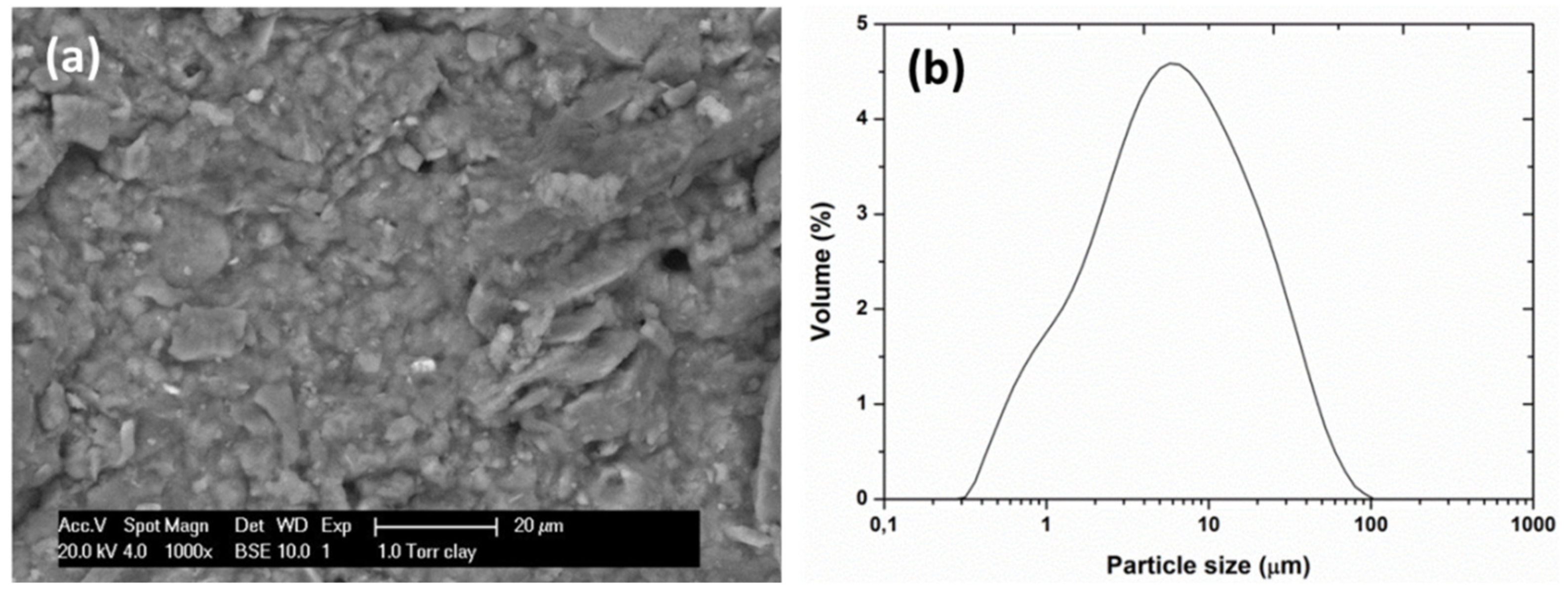
2.1. Clay
2.2. Flocculant
2.3. Solvent
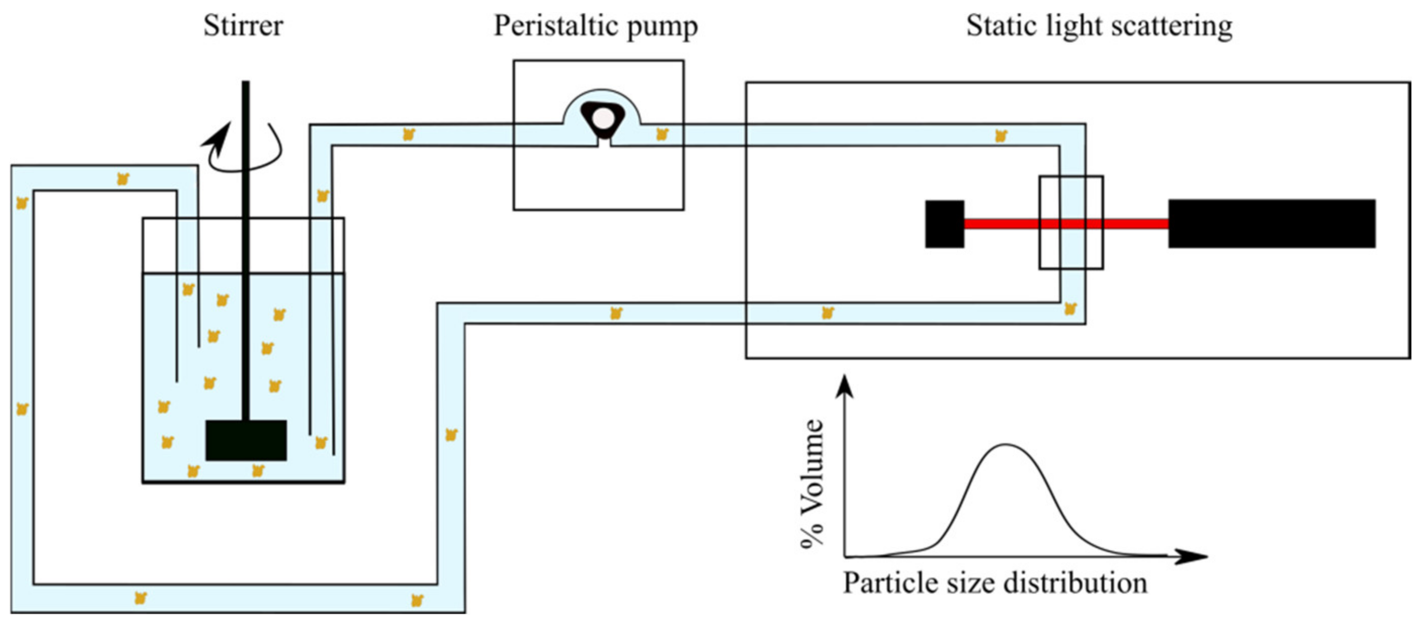
2.4. Static Light Scattering Experiments
2.4.1. Particle (Floc) Size Distribution
2.4.2. Shear Stress Experiments
2.5. Settling Column Experiments
2.6. Electrophoretic Mobility and -Potential
2.7. Rheological Measurements
3. Results and Discussion
3.1. Static Light Scattering (SLS) Measurements
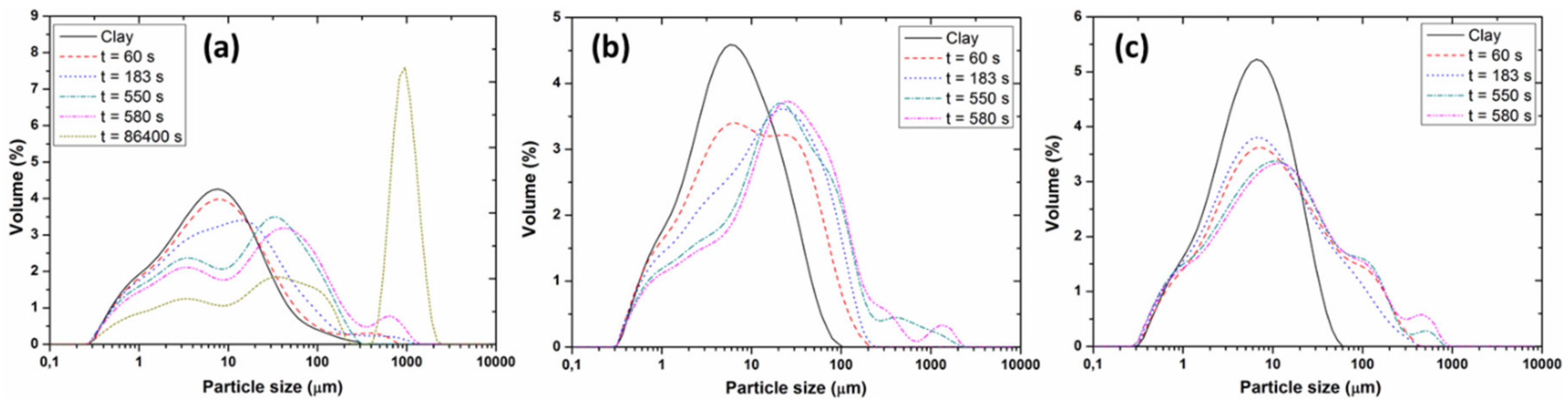
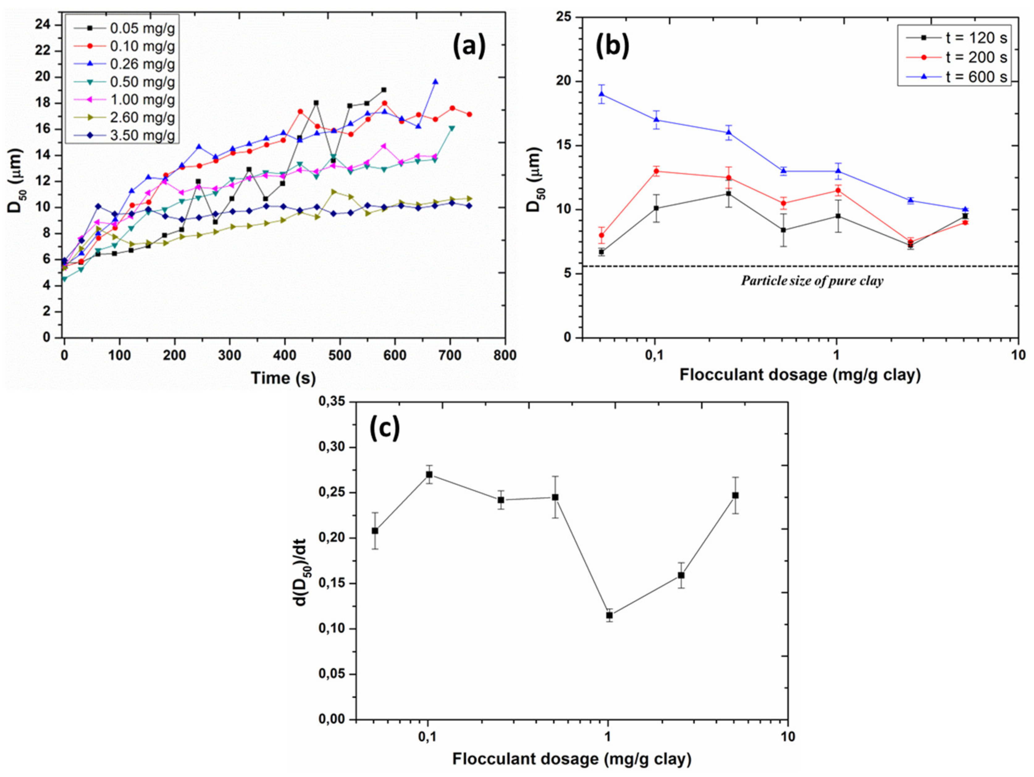
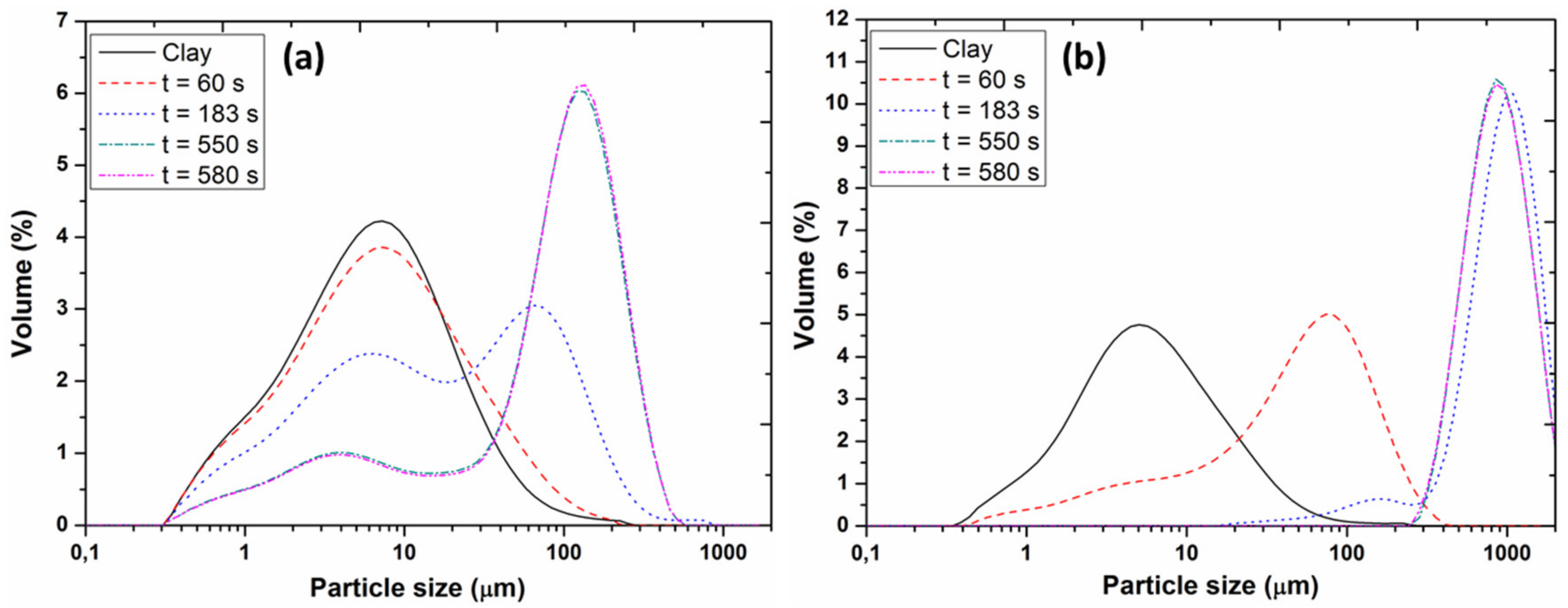
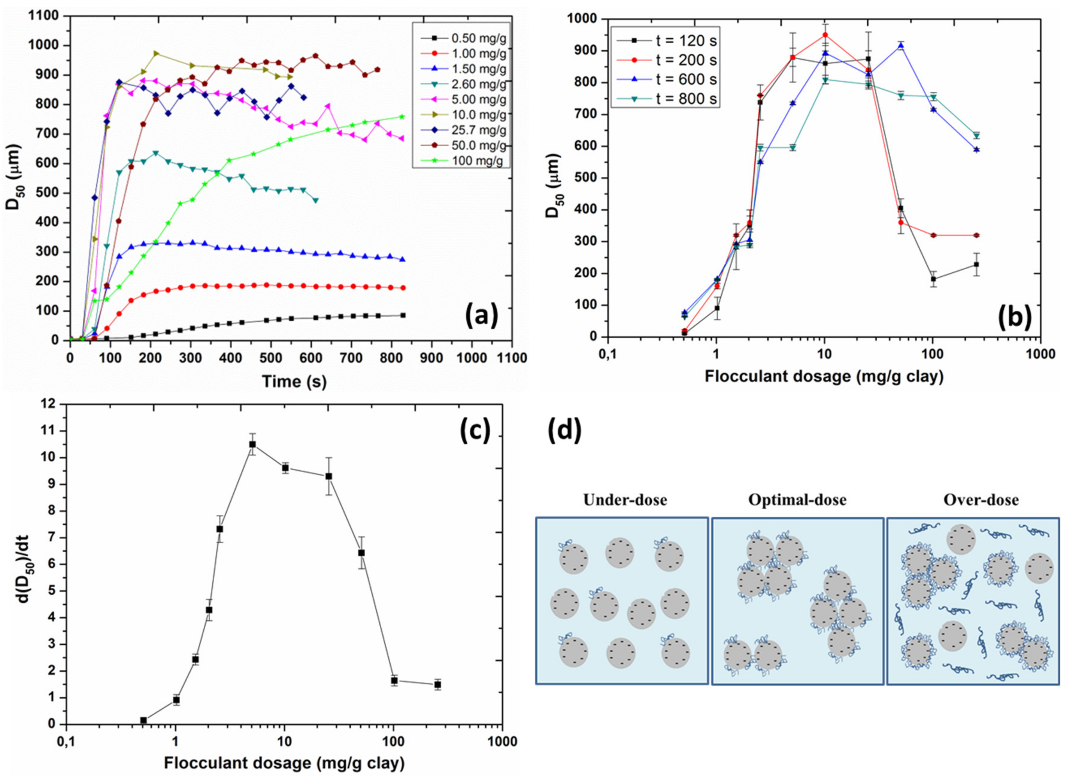
3.1.1. Particle Size Evolution as a Function of Time
Anionic Flocculant
Cationic Flocculant
3.1.2. Reversibility Upon Shear
Anionic Flocculant
- Flocs created at a lower shear rate were large, i.e., about 1 mm (filled squares in Figure 7) and their dependence on the shear rate was nearly completely reversible, as indicated by the empty squares in Figure 7. Only for the lowest shear rates the flocs regrew to half of their original size (i.e., about 500 µm).
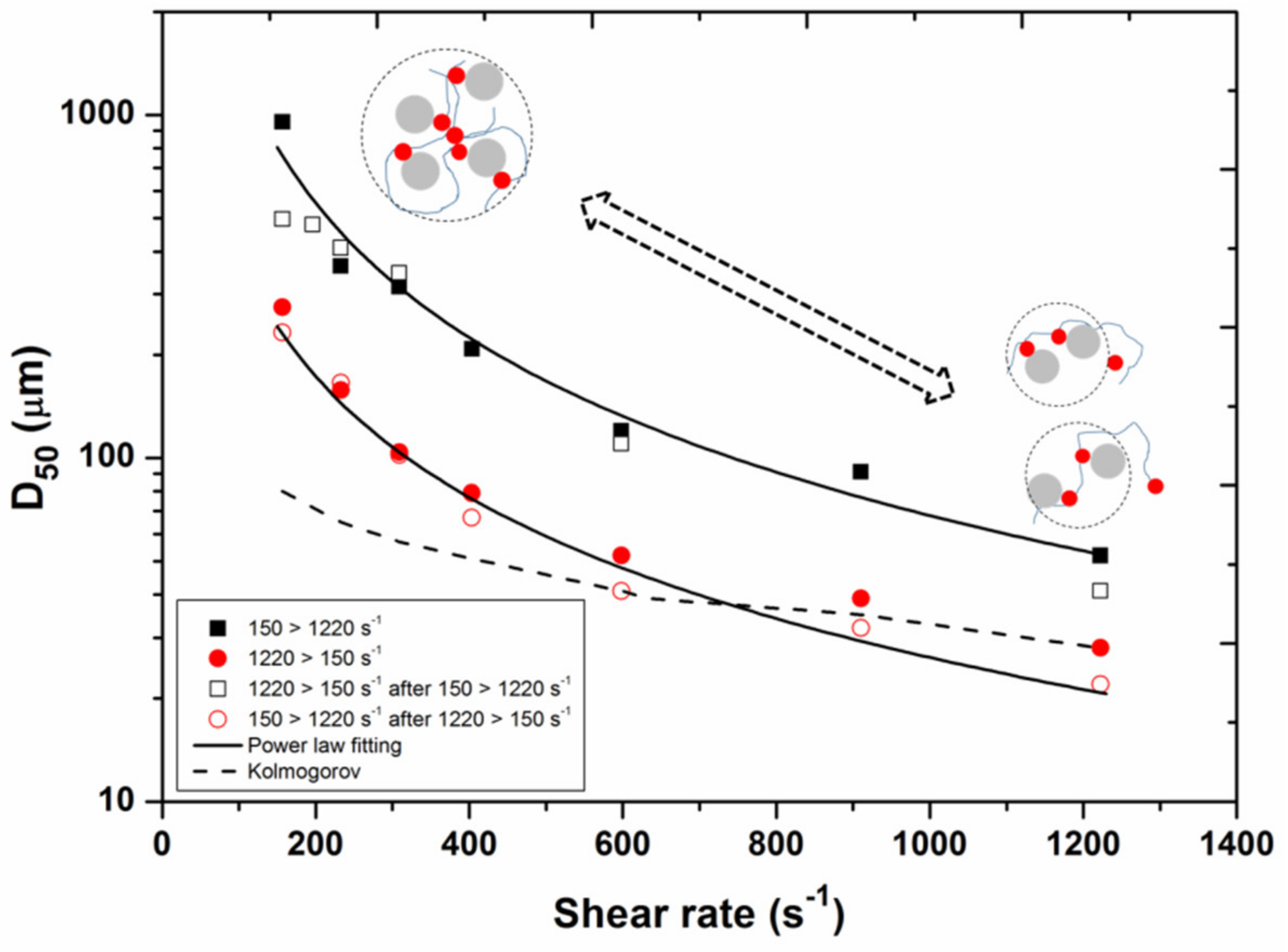
Cationic Flocculant
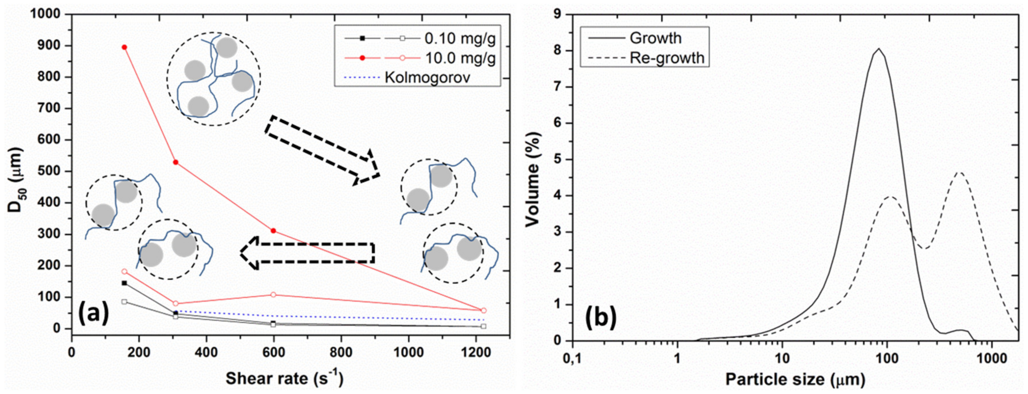
- At underdose flocculant (0.1 mg/g) the flocs created were small and close to the Kolmogorov length. The flocs regrew to their initial steady-state value upon a decrease in shear, except at the lowest measured shear, where they regrew to a size of 86 microns instead of a size of 145 microns.
3.2. Settling Column Measurements
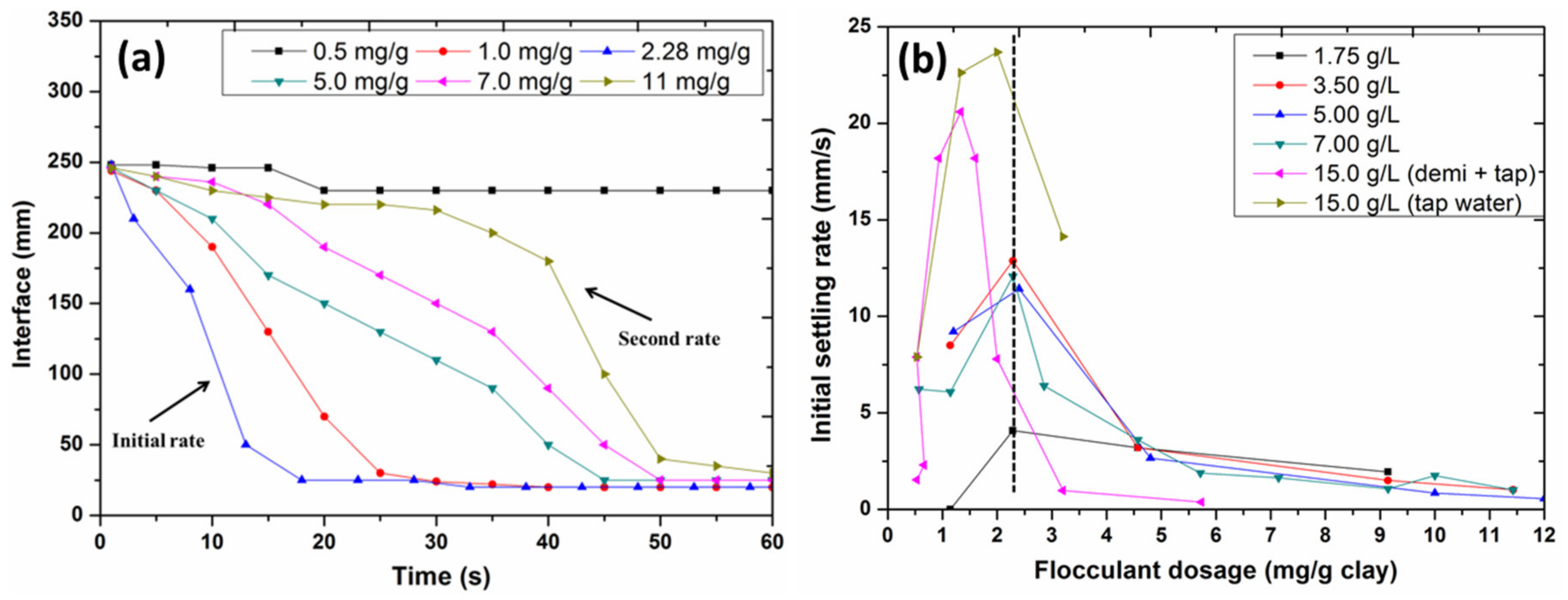
3.2.1. Anionic Flocculant
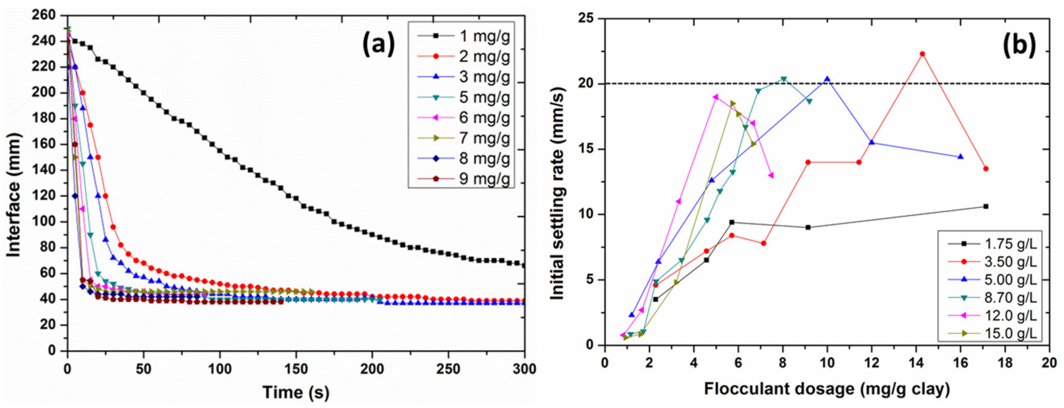
3.2.2. Cationic Flocculant
3.3. Electrophoretic Mobility Measurements
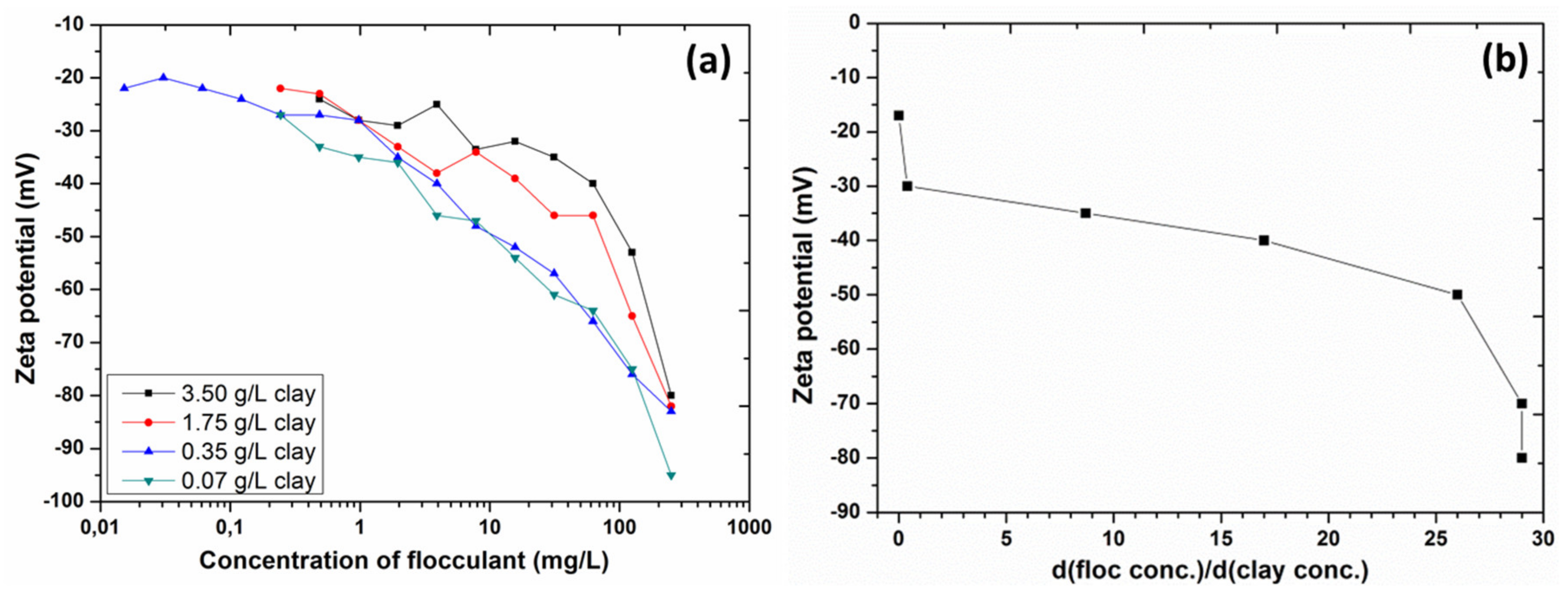
3.3.1. Anionic Flocculant
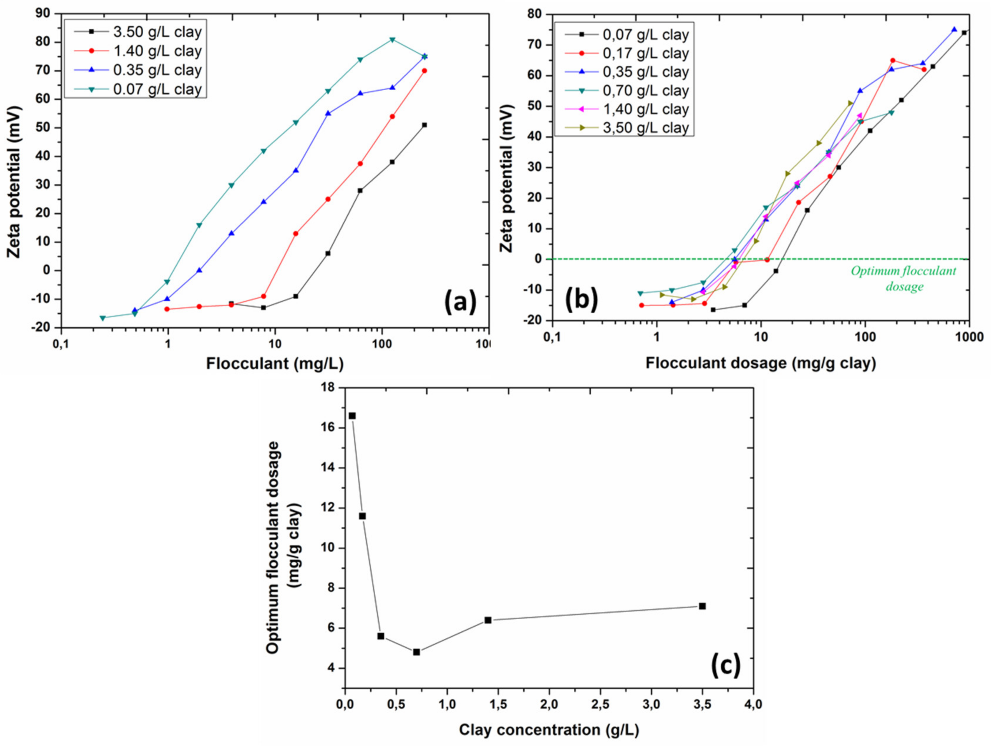
3.3.2. Cationic Flocculant
3.4. Rheological Analysis
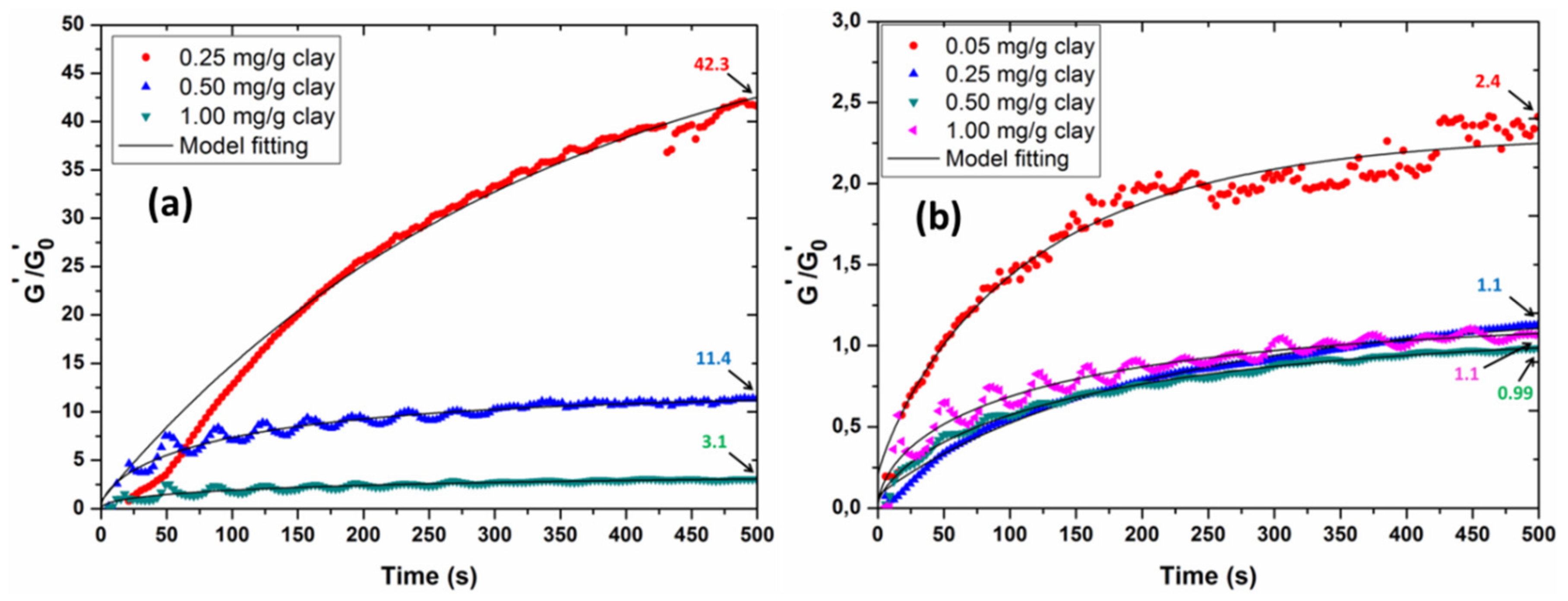
3.4.1. Anionic Flocculant
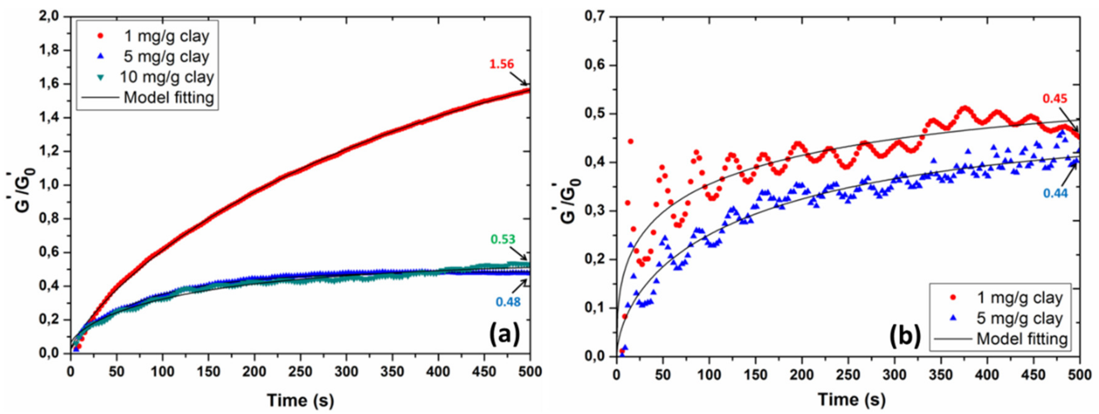
3.4.2. Cationic Flocculant
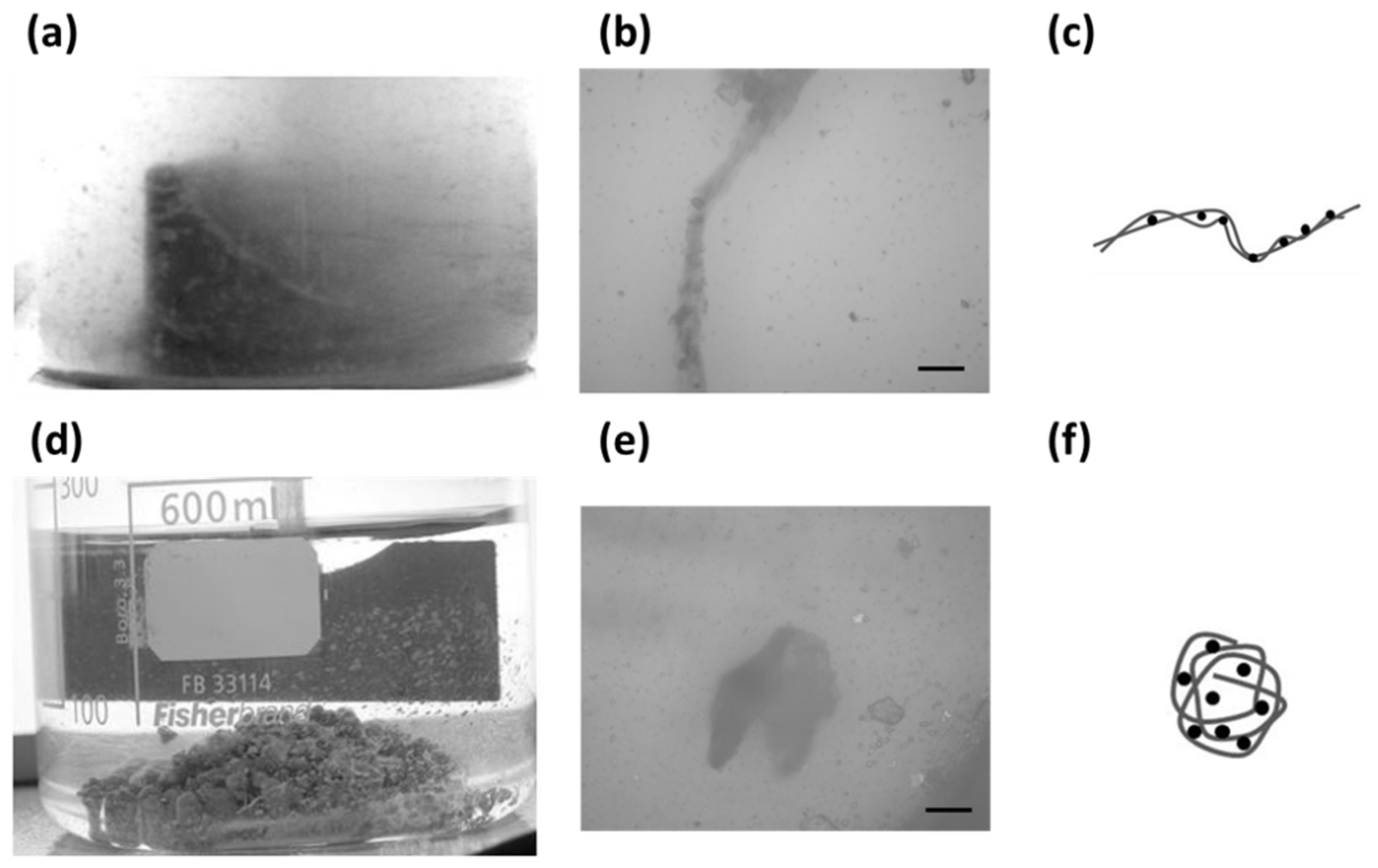
3.5. (Micro) Structural Observations
3.6. Discussion
3.6.1. Anionic Flocculant
3.6.2. Cationic Flocculant
4. Conclusions
- The presence of cations in the water was determinant for the flocculation efficiency and flocculation dynamics of clay in the presence of anionic polyelectrolyte. The shape of the flocs was found to be very elongated in cation-poor water. It remains to be investigated how this conformation would change in saline water, and how the flocculation dynamics would be affected. Preliminary studies have shown that the order in which the polyanionic flocculant, clay and electrolyte are mixed has a large influence on the obtained flocs. This is of particular importance for estuarine conditions, where changes from fresh to saline water take place. Even though it is not discussed in the present article, the fact that particles are elongated also lead to problems in the analysis of the light scattering data, as most software are made for the analysis of spherical shaped objects. It is known that the interpretation of in-situ light scattering data is in particular affected by the presence of elongated particles.
- The size of flocs obtained by the anionic flocculant is reversible upon shear, implying that these are independent of shear history. The main reason for this reversibility is that the clay and polyelectrolyte attach through cation bridging, which is a weak interaction. It remains to be seen, in the case of natural polyanions, like humic substances of low to moderate molecular weight (which can be surface active), if other forces for instance steric forces could play an additional role and lead to different aggregate structures and flocs of different sizes and strength.
- The large flocs obtained by the cationic flocculant were formed by a strong electrostatic attraction and their shape and size was extremely shear-dependent, making them history dependent: their properties depend not only on the shear level but also on the time that a given shear is applied. The fact that flocs can reconform under shear, i.e., become denser without loss of clay and polymer mass, has consequences in terms of modelling, as aggregation models are based on the fact that particles can change their size upon aggregation or break-up but not because of a change in volume without a loss of mass.
Supplementary Materials
Author Contributions
Funding
Acknowledgments
Conflicts of Interest
References
- Liss, S.N.; Milligan, T.G.; Droppo, I.G.; Leppard, G.G. Methods for analyzing floc properties. In Flocculation in Natural and Engineered Environmental Systems; CRC Press: Boca Raton, FL, USA, 2005. [Google Scholar]
- Manning, A.; Baugh, J.; Soulsby, R.; Spearman, J.; Whitehouse, R. Cohesive sediment flocculation and the application to settling flux modelling. In Sediment Transport; Ginsberg, S.S., Ed.; IntechOpen: Rijeka, Croatia, 2011; pp. 91–116. [Google Scholar]
- Bergaya, F.; Lagaly, G. Handbook of Clay Science; Newnes: Amsterdam, The Netherland, 2013; Volume 5. [Google Scholar]
- Lee, B.J.; Schlautman, M.A.; Toorman, E.; Fettweis, M. Competition between kaolinite flocculation and stabilization in divalent cation solutions dosed with anionic polyacrylamides. Water Res. 2012, 46, 5696–5706. [Google Scholar] [CrossRef]
- Mietta, F.; Chassagne, C.; Winterwerp, J.C. Shear-induced flocculation of a suspension of kaolinite as function of pH and salt concentration. J. Colloid Interface Sci. 2009, 336, 134–141. [Google Scholar] [CrossRef] [PubMed]
- Tan, X.-l.; Zhang, G.-p.; Yin, H.; Reed, A.H.; Furukawa, Y. Characterization of particle size and settling velocity of cohesive sediments affected by a neutral exopolymer. Int. J. Sediment Res. 2012, 27, 473–485. [Google Scholar] [CrossRef]
- Bolto, B.; Gregory, J. Organic polyelectrolytes in water treatment. Water Res. 2007, 41, 2301–2324. [Google Scholar] [CrossRef] [PubMed]
- Concha Arcil, F. Settling Velocities of Particulate Systems. Kona Powder Part. J. 2009, 27, 18–37. [Google Scholar] [CrossRef] [Green Version]
- Mierczynska-Vasilev, A.; Kor, M.; Addai-Mensah, J.; Beattie, D.A. The influence of polymer chemistry on adsorption and flocculation of talc suspensions. Chem. Eng. J. 2013, 220, 375–382. [Google Scholar] [CrossRef]
- Goodwin, J. Colloids and Interfaces with Surfactants and Polymers; John Wiley & Sons: West Sussex, UK, 2009. [Google Scholar]
- Barany, S.; Meszaros, R.; Kozakova, I.; Skvarla, I. Kinetics and mechanism of flocculation of bentonite and kaolin suspensions with polyelectrolytes and the strength of floccs. Colloid J. 2009, 71, 285–292. [Google Scholar] [CrossRef]
- Barany, S.; Kozakova, I.; Marcinova, L.; Skvarla, J. Electrokinetic potential of bentonite and kaolin particles in the presence of polymer mixtures. Colloid J. 2010, 72, 595–601. [Google Scholar] [CrossRef]
- Bárány, S.; Meszaros, R.; Marcinova, L.; Skvarla, J. Effect of polyelectrolyte mixtures on the electrokinetic potential and kinetics of flocculation of clay mineral particles. Colloids Surf. A Physicochem. Eng. Asp. 2011, 383, 48–55. [Google Scholar] [CrossRef]
- Stewart, C.; Thompson, J.A.J. Vertical Distribution of Butyltin Residues in Sediments of British Columbia Harbours. Environ. Technol. 1997, 18, 1195–1202. [Google Scholar] [CrossRef]
- McLaughlin, R.A.; Bartholomew, N. Soil factors influencing suspended sediment flocculation by polyacrylamide. Soil Sci. Soc. Am. J. 2007, 71, 537–544. [Google Scholar]
- Sojka, R.E.; Bjorneberg, D.L.; Entry, J.A.; Lentz, R.D.; Orts, W.J. Polyacrylamide in Agriculture and Environmental Land Management. In Advances in Agronomy; Sparks, D.L., Ed.; Academic Press: Cambridge, MA, USA, 2007; Volume 92, pp. 75–162. [Google Scholar]
- Mietta, F.; Maggi, F.; Winterwerp, J.C. Chapter 19 Sensitivity to breakup functions of a population balance equation for cohesive sediments. In Proceedings in Marine Science; Kusuda, T., Yamanishi, H., Spearman, J., Gailani, J.Z., Eds.; Elsevier: Amsterdam, The Netherlands, 2008; Volume 9, pp. 275–286. [Google Scholar]
- Malvern. Available online: www.malvern.com (accessed on 10 April 2020).
- Bouyer, D.; Coufort, C.; Liné, A.; Do-Quang, Z. Experimental analysis of floc size distributions in a 1-L jar under different hydrodynamics and physicochemical conditions. J. Colloid Interface Sci. 2005, 292, 413–428. [Google Scholar] [CrossRef] [PubMed]
- Hunter, R.J. Zeta Potential in Colloid Science: Principles and Applications; Academic Press: London, UK, 1981; Volume 2. [Google Scholar]
- Chassagne, C.; Ibanez, M. Hydrodynamic size and electrophoretic mobility of latex nanospheres in monovalent and divalent electrolytes. Colloids Surf. A Physicochem. Eng. Asp. 2014, 440, 208–216. [Google Scholar] [CrossRef]
- Shakeel, A.; Kirichek, A.; Chassagne, C. Effect of pre-shearing on the steady and dynamic rheological properties of mud sediments. Mar. Pet. Geol. 2020, 116, 104338. [Google Scholar] [CrossRef]
- Gregory, J. Rates of flocculation of latex particles by cationic polymers. J. Colloid Interface Sci. 1973, 42, 448–456. [Google Scholar] [CrossRef]
- Mpofu, P.; Addai-Mensah, J.; Ralston, J. Investigation of the effect of polymer structure type on flocculation, rheology and dewatering behaviour of kaolinite dispersions. Int. J. Miner. Process. 2003, 71, 247–268. [Google Scholar] [CrossRef]
- Mpofu, P.; Addai-Mensah, J.; Ralston, J. Flocculation and dewatering behaviour of smectite dispersions: Effect of polymer structure type. Miner. Eng. 2004, 17, 411–423. [Google Scholar] [CrossRef]
- Sworska, A.; Laskowski, J.S.; Cymerman, G. Flocculation of the Syncrude fine tailings: Part I. Effect of pH, polymer dosage and Mg2+ and Ca2+ cations. Int. J. Miner. Process. 2000, 60, 143–152. [Google Scholar] [CrossRef]
- Sworska, A.; Laskowski, J.S.; Cymerman, G. Flocculation of the Syncrude fine tailings: Part II. Effect of hydrodynamic conditions. Int. J. Miner. Process. 2000, 60, 153–161. [Google Scholar] [CrossRef]
- Bubakova, P.; Pivokonsky, M.; Filip, P. Effect of shear rate on aggregate size and structure in the process of aggregation and at steady state. Powder Technol. 2013, 235, 540–549. [Google Scholar] [CrossRef]
- Mietta, F. Evolution of the Floc Size Distribution of Cohesive Sediments. Ph.D. Thesis, Delft University of Technology, Delft, The Netherlands, 2010. [Google Scholar]
- Yoon, S.-Y.; Deng, Y. Flocculation and reflocculation of clay suspension by different polymer systems under turbulent conditions. J. Colloid Interface Sci. 2004, 278, 139–145. [Google Scholar] [CrossRef] [PubMed]
- Zhao, Y.Q. Settling behaviour of polymer flocculated water-treatment sludge I: Analyses of settling curves. Sep. Purif. Technol. 2004, 35, 71–80. [Google Scholar] [CrossRef] [Green Version]
- Chen, G.W.; Chang, I.L.; Hung, W.T.; Lee, D.J. Regimes for zone settling of waste activated sludges. Water Res. 1996, 30, 1844–1850. [Google Scholar] [CrossRef]
- Fargues, C.; Turchiuli, C. Structural Characterization of Flocs in Relation to Their Settling Performances. Chem. Eng. Res. Des. 2003, 81, 1171–1178. [Google Scholar] [CrossRef]
- Owen, A.T.; Fawell, P.D.; Swift, J.D.; Labbett, D.M.; Benn, F.A.; Farrow, J.B. Using turbulent pipe flow to study the factors affecting polymer-bridging flocculation of mineral systems. Int. J. Miner. Process. 2008, 87, 90–99. [Google Scholar] [CrossRef]
- Wen, H.J.; Liu, C.I.; Lee, D.J. Size and density of flocculated sludge flocs. J. Environ. Sci. Health. Part A Environ. Sci. Eng. Toxicol. 1997, 32, 1125–1137. [Google Scholar] [CrossRef]
- Grasso, D.; Subramaniam, K.; Butkus, M.; Strevett, K.; Bergendahl, J. A review of non-DLVO interactions in environmental colloidal systems. Rev. Environ. Sci. Biotechnol. 2002, 1, 17–38. [Google Scholar] [CrossRef]
- Li, F.; Allison, S.A.; Hill, R.J. Nanoparticle gel electrophoresis: Soft spheres in polyelectrolyte hydrogels under the Debye–Hückel approximation. J. Colloid Interface Sci. 2014, 423, 129–142. [Google Scholar] [CrossRef]
- Petzold, G.; Nebel, A.; Buchhammer, H.-M.; Lunkwitz, K. Preparation and characterization of different polyelectrolyte complexes and their application as flocculants. Colloid Polym. Sci. 1998, 276, 125–130. [Google Scholar] [CrossRef]
- Petzold, G.; Mende, M.; Lunkwitz, K.; Schwarz, S.; Buchhammer, H.M. Higher efficiency in the flocculation of clay suspensions by using combinations of oppositely charged polyelectrolytes. Colloids Surf. A Physicochem. Eng. Asp. 2003, 218, 47–57. [Google Scholar] [CrossRef]
- Goudoulas, T.B.; Germann, N. Viscoelastic properties of polyacrylamide solutions from creep ringing data. J. Rheol. 2016, 60, 491–502. [Google Scholar] [CrossRef]
- Shakeel, A.; van Kan, P.J.M.; Chassagne, C. Design of a parallel plate shearing device for visualization of concentrated suspensions. Measurement 2019, 145, 391–399. [Google Scholar] [CrossRef]
- Borkovec, M.; Behrens, S.H.; Semmler, M. Observation of the Mobility Maximum Predicted by the Standard Electrokinetic Model for Highly Charged Amidine Latex Particles. Langmuir 2000, 16, 5209–5212. [Google Scholar] [CrossRef]
- Narkis, N.; Ghattas, B.; Rebhun, M.; Rubin, A. Mechanism of flocculation with aluminium salts in combination with polymeric flocculants as flocculant aids. Water Supply 1991, 9, 37–44. [Google Scholar]
- Barnes, H.A. A review of the slip (wall depletion) of polymer solutions, emulsions and particle suspensions in viscometers: Its cause, character, and cure. J. Nonnewton Fluid Mech. 1995, 56, 221–251. [Google Scholar] [CrossRef]
- Chassagne, C. Understanding the natural consolidation of slurries using colloid science. In Proceedings of the European Conference on Soil Mechanics and Geotechnical Engineering, Reykjavik, Iceland, 1–6 September 2019. [Google Scholar]
- Dhont, J.K. An Introduction to Dynamics of Colloids; Elsevier: Amsterdam, The Netherlands, 1996. [Google Scholar]
- Faas, R.W.; Wartel, S.I. Rheological properties of sediment suspensions from Eckernförde and Kieler Förde Bays, western Baltic Sea. Int. J. Sediment Res. 2006, 21, 24–41. [Google Scholar]
- Huang, Z.; Aode, H. A laboratory study of rheological properties of mudflows in Hangzhou Bay, China. Int. J. Sediment Res. 2009, 24, 410–424. [Google Scholar] [CrossRef] [Green Version]
- Kanai, H.; Navarrete, R.C.; Macosko, C.W.; Scriven, L.E. Fragile networks and rheology of concentrated suspensions. Rheol. Acta 1992, 31, 333–344. [Google Scholar] [CrossRef]
- Koumakis, N.; Petekidis, G. Two step yielding in attractive colloids: Transition from gels to attractive glasses. Soft Matter 2011, 7, 2456–2470. [Google Scholar] [CrossRef]
- Kramb, R.C.; Zukoski, C.F. Yielding in dense suspensions: Cage, bond, and rotational confinements. J. Phys. Condens. Matter 2010, 23, 035102. [Google Scholar] [CrossRef]
- Maranzano, B.J.; Wagner, N.J. The effects of interparticle interactions and particle size on reversible shear thickening: Hard-sphere colloidal dispersions. J. Rheol. 2001, 45, 1205–1222. [Google Scholar] [CrossRef] [Green Version]
- Mewis, J.; Wagner, N.J. Colloidal Suspension Rheology; Cambridge University Press: Cambridge, UK, 2012. [Google Scholar]
- Mobuchon, C.; Carreau, P.J.; Heuzey, M.-C. Structural analysis of non-aqueous layered silicate suspensions subjected to shear flow. J. Rheol. 2009, 53, 1025–1048. [Google Scholar] [CrossRef] [Green Version]
- O’Brien, J.S.; Julien, P.Y. Laboratory Analysis of Mudflow Properties. J. Hydraul. Eng. 1988, 114, 877–887. [Google Scholar] [CrossRef] [Green Version]
- Richardson, J.F.; Zaki, W.N. The sedimentation of a suspension of uniform spheres under conditions of viscous flow. Chem. Eng. Sci. 1954, 3, 65–73. [Google Scholar] [CrossRef]
- Shakeel, A.; Kirichek, A.; Chassagne, C. Is density enough to predict the rheology of natural sediments? Geo-Marine Letters 2019, 39, 427–434. [Google Scholar] [CrossRef] [Green Version]
- Shakeel, A.; Kirichek, A.; Chassagne, C. Rheological analysis of mud from Port of Hamburg, Germany. J. Soils Sediments. 2020, 20, 2553–2562. [Google Scholar] [CrossRef] [Green Version]
- Soltanpour, M.; Samsami, F. A comparative study on the rheology and wave dissipation of kaolinite and natural Hendijan Coast mud, the Persian Gulf. Ocean Dyn. 2011, 61, 295–309. [Google Scholar] [CrossRef]
- Van Kessel, T.; Blom, C. Rheology of cohesive sediments: Comparison between a natural and an artificial mud. J. Hydraul. Res. 1998, 36, 591–602. [Google Scholar] [CrossRef]
- Xu, J.; Huhe, A. Rheological study of mudflows at Lianyungang in China. Int. J. Sediment Res. 2016, 31, 71–78. [Google Scholar] [CrossRef]
- Zhu, L.; Sun, N.; Papadopoulos, K.; Kee, D.D. A slotted plate device for measuring static yield stress. J. Rheol. 2001, 45, 1105–1122. [Google Scholar] [CrossRef]


| Mineral | Weight % |
|---|---|
| Quartz | 24.0 |
| Alkali Feldspar | 3.5 |
| Plagioclase | 4.0 |
| Calcite | 9.6 |
| Mg-Calcite | 2.9 |
| Aragonite | 2.7 |
| Dolomite | 0.6 |
| Ankerite | 0.2 |
| Rutile | 0.1 |
| Anatase | 0.1 |
| Gypsum | 0.1 |
| Pyrite | 0.6 |
| Halite | 0.8 |
| Kaolinitic | 3.2 |
| Chloritic | 1.2 |
| 2:1 Layer silicates | 46.5 |
| Parameter | Value | Units |
|---|---|---|
| pH | 8.2–8.7 | - |
| Bicarbonate | 188–225 | mg/L |
| Sulphate | 24–30 | mg/L |
| Sodium | 51–59 | mg/L |
| Calcium | 45–49 | mg/L |
| Magnesium | 8.2–8.4 | mg/L |
| Chloride | 48.6–49.1 | mg/L |
| Flocculant Dosage | Standard Error | Standard Error | (-) | Standard Error | |||
|---|---|---|---|---|---|---|---|
| 30 wt % clay | |||||||
| 0.25 mg/g clay | 421 | 3.1 | 334 | 24 | 0.99 | 0.04 | 55 |
| 0.5 mg/g clay | 1098 | 21.2 | 115 | 6 | 0.64 | 0.02 | 12 |
| 1 mg/g clay | 1511 | 33.6 | 230 | 16 | 0.52 | 0.01 | 4 |
| 40 wt % clay | |||||||
| 0.05 mg/g clay | 266 | 1.7 | 117 | 5 | 0.86 | 0.03 | 2.3 |
| 0.25 mg/g clay | 378 | 2.8 | 213 | 15 | 0.94 | 0.03 | 1.2 |
| 0.5 mg/g clay | 888 | 15.8 | 165 | 17 | 0.70 | 0.02 | 1.1 |
| 1 mg/g clay | 1799 | 36.5 | 136 | 6 | 0.60 | 0.01 | 1.2 |
| Flocculant Dosage | Standard Error | Standard Error | (-) | Standard Error | |||
|---|---|---|---|---|---|---|---|
| 30 wt % clay | |||||||
| 1 mg/g clay | 1866 | 38.1 | 448 | 35 | 0.82 | 0.03 | 2.31 |
| 5 mg/g clay | 14,142 | 654.2 | 79 | 5 | 0.85 | 0.03 | 0.50 |
| 10 mg/g clay | 27,774 | 1129.4 | 146 | 8 | 0.72 | 0.02 | 0.55 |
| 40 wt % clay | |||||||
| 1 mg/g clay | 5914 | 195.4 | 134 | 6 | 0.40 | 0.01 | 0.59 |
| 5 mg/g clay | 18,306 | 845.3 | 163 | 17 | 0.61 | 0.02 | 0.48 |
Publisher’s Note: MDPI stays neutral with regard to jurisdictional claims in published maps and institutional affiliations. |
© 2020 by the authors. Licensee MDPI, Basel, Switzerland. This article is an open access article distributed under the terms and conditions of the Creative Commons Attribution (CC BY) license (http://creativecommons.org/licenses/by/4.0/).
Share and Cite
Shakeel, A.; Safar, Z.; Ibanez, M.; van Paassen, L.; Chassagne, C. Flocculation of Clay Suspensions by Anionic and Cationic Polyelectrolytes: A Systematic Analysis. Minerals 2020, 10, 999. https://0-doi-org.brum.beds.ac.uk/10.3390/min10110999
Shakeel A, Safar Z, Ibanez M, van Paassen L, Chassagne C. Flocculation of Clay Suspensions by Anionic and Cationic Polyelectrolytes: A Systematic Analysis. Minerals. 2020; 10(11):999. https://0-doi-org.brum.beds.ac.uk/10.3390/min10110999
Chicago/Turabian StyleShakeel, Ahmad, Zeinab Safar, Maria Ibanez, Leon van Paassen, and Claire Chassagne. 2020. "Flocculation of Clay Suspensions by Anionic and Cationic Polyelectrolytes: A Systematic Analysis" Minerals 10, no. 11: 999. https://0-doi-org.brum.beds.ac.uk/10.3390/min10110999