Article

Effect of the Fracturing Degree of the Source Rock on Rock Avalanche River-Blocking Behavior Based on the Coupled Eulerian-Lagrangian Technique

1
Key Laboratory of Mountain Hazards and Earth Surface Process, Institute of Mountain Hazards and Environment, Chinese Academy of Sciences, Chengdu 610041, China
2
College of Construction Engineering, Jilin University, Changchun 130026, China
3
DongChen International School, Chengdu 621051, China
*
Author to whom correspondence should be addressed.
Submission received: 15 June 2022 / Revised: 11 July 2022 / Accepted: 14 July 2022 / Published: 18 July 2022
(This article belongs to the Section Clays and Engineered Mineral Materials)

Abstract

:
In this study, the effect of the fracturing degree of the source rock on rock avalanche river-blocking behavior was investigated. The study included the analysis of mass movement behavior, impulse wave behavior, and the formation of landslide dams. The study included a series of simulations of rock avalanche river-blocking based on the coupled Eulerian-Lagrangian (CEL) technique. Prior to the simulation, a water column collapse model was applied to validate the use of the CEL technique on fluid-structure interaction, and to calibrate the material parameters. The source rock in the rock avalanche simulation was cut by different groups of structural planes, with the number of 0 × 0 × 0, 1 × 1 × 1, 4 × 4 × 4, 9 × 9 × 9, 14 × 14 × 14, 19 × 19 × 19 in each dimension, respectively, to represent different fracturing degrees, on the premise of the same volume and shape of the source rock. The simulation results showed that the sliding mass exhibited structure stabilization, such that the structure of the sliding mass gradually stabilized to a steady status over time, in the mass movement process. The structure stabilization made the center of the sliding mass constantly decrease, and provided a higher speed of movement for the rock avalanches with higher fracturing degrees of the source rock. As for the impulse wave behavior, with the increase in the fracturing degree of the source rock, the maximum kinetic energy of the water decreased, and the maximum height and propagation speed of the impulse waves decreased, which indicated that the maximum height and the propagation speed of the impulse waves were positively correlated with the maximum kinetic energy of the water. In regard to the formation of the landslide dams, when the fracturing degree of the source rock was low, the shape of the landslide dam was very different. With the increase of the fracturing degree of the source rock, the shapes of the landslide dams stabilized, and varied slightly after the fracturing degree of the source rock reached a threshold value.

1. Introduction

Rock avalanches frequently occur in valleys, and lead to river-blocking [1,2,3,4]. As a result, they usually generate disaster chains that include rock avalanches, impulse waves, and landslide dams [5,6,7]. Each disaster in the chain can cause significant threats to human lives and property. The whole process of disaster chains is complex, and has become a hot topic in the last few decades. In a disaster chain, the rock avalanche is the first disaster, and plays a crucial role in the subsequent disaster behavior. Several factors, including the material characteristics of the source and the path [8,9], the source volume [10,11,12], and the topography [13,14], influence the behavior of the runout of rock avalanches. However, the fracturing degree of the source rock, and its influence on the landslide river blocking, is rarely systematically studied. Rock masses in valleys frequently have very different fracturing degrees (Figure 1). Some cases of landslides [15,16] have indicated that the high fracturing degree of the source rock can lead to an unusually long runout distance, and can affect the post-failure disaster behavior, such as landslide-induced impulse waves [17,18] and dam failures ([1]). Therefore, it is necessary to study the effect of the fracturing degree of the source rock on the rock avalanche runout behavior and subsequent disasters.
Detailed processes deep in a moving rock avalanche can only be speculated, rather than directly observed, which makes it difficult to conduct this kind of research. Although some studies have conducted laboratory experiments to investigate the influence of source structure on runout behavior and the formation of landslide dams [19,20], the scale of laboratory experiments differs from real cases of rock avalanches, and the obtained parameters may be scale-dependent [21,22]. Furthermore, from laboratory experiments, it is difficult to obtain information about the velocity and force of blocks. Therefore, it has proved necessary to conduct numerical studies on the effects of the fracturing degree of the source rock on the behavior of rock avalanches and post-failure disasters. Over the past few years, several methods have been used to simulate slope failure and rock avalanches, including: the finite element method (FEM) [9,23]; the discrete element method (DEM) [24,25]; discontinuous deformation analysis (DDA) [26,27]; smoothed particle hydrodynamics (SPH) [28,29]; the material point method (MPM) [30]; the shallow water model (SWM) [31,32]; and the moving particle simulation (MPS) [33,34]. However, it is difficult to show the fracturing degree of the source rock using a continuum method such as SWM. In addition, previous studies have focused mainly on the runout behavior of rock avalanches, ignoring the simulation of other disasters in the chain. This is because simulation of the interaction between the fluid and the structure (i.e., the sliding mass and the river) is still a challenging task. The approach to the simulation of the landslide disaster chain in previous studies [9,15] was to integrate the simulation of a single disaster; but a method that can fully reflect the entire process of landslide river-blocking is desirable.
To investigate the effect of the fracturing degree of the source rock on the entire river-blocking behavior, the coupled Eulerian-Lagrangian (CEL) method was used in this study. The combined CEL method has the advantages of both the Lagrangian method and the Eulerian method, and at the same time can capture the precise strain field on the Lagrangian meshes, and the large deformation characteristics of the materials in the Euler meshes [24,35]. The CEL method can be used to simulate a rock avalanche by placing rock bodies as discrete Lagrangian blocks, and it can also solve the problem of the fluid-structure coupling. It is a potentially innovative and valuable method for simulating landslide river-blocking. In this study, a series of numerical models of rock avalanches based on the CEL method were used to investigate the effects of the fracturing degree of the source rock on rock avalanche river-blocking behavior. The source rock was cut by discontinuous structural planes, and the total dimension of each cut source rock was 25 × 25 × 25 m3. The number of structural planes in each group of models was set at 0 × 0 × 0, 1 × 1 × 1, 4 × 4 × 4, 9 × 9 × 9, 14 × 14 × 14, 19 × 19 × 19 in each dimension, and the number of potential breakage blocks was 1, 8, 125, 1000, 3375, and 8000, respectively, in order to represent the different fracturing degrees of the cut source rocks. The whole process was observed, including the rock sliding along the slope, running into the river, and forming a landslide dam. Furthermore, the effects of the different fracturing degrees of the cut source rocks on sliding mobility, impulse wave behavior, and formation of the landslide dam, were studied.

2. Methodology

2.1. CEL Technique

The traditional Lagrangian method is widely used for the analysis of solid materials. In the traditional Lagrangian method, nodes are fixed with material, and the elements are always full of individual materials, making the meshes deform as the material deforms (Figure 2a). Although accurate numerical solutions can be obtained using the Lagrange method, it has limitations in the analysis of elements with large deformations due to mesh distortion. In contrast, the Eulerian method is used to analyze large deformations. Nodes in the Eulerian method are always fixed in space. The material flows through the fixed elements, making the material boundary and the Eulerian volume fraction of the material in the meshes vary with increase in time (Figure 2b). The Eulerian volume fraction is defined as the percentage of the region occupied by a particular material. The Eulerian method can be applied to the analysis of large deformations because the material is independent on the meshes, and the calculation cannot be divergent due to the mesh distortion. However, the accuracy of the Eulerian method for capturing the geometric boundary of the model is lower than that of the Lagrangian method. The CEL method has the advantages of both the traditional Lagrangian method and the Eulerian method, in that small deformed parts can be modeled by Lagrangian elements while large deformed parts can be modeled by Eulerian elements at the same time. The Lagrangian elements will move freely in the Eulerian mesh until the elements encounter a Eulerian part filled with material (Figure 3a). In each computational step, the Lagrangian method calculates the node displacement, velocity, force, and other variables of the Lagrangian element, according to the governing equation. The Eulerian method calculates the pressure, density, and internal energy of the Eulerian element. The Eulerian elements transfer the pressure to the coupling interface, and distribute the nodal load to the Lagrangian element on the coupling interface. Then, the Lagrangian elements calculate the displacement of the nodes, and update the position of the coupling interface, thus changing the Eulerian volume fraction of material, velocity, and pressure in the Eulerian mesh (Figure 3b). The above-mentioned steps are repeated throughout the calculation process until the calculation is stopped.

2.2. Governing Equation of Material

In the simulation, the rock body was defined as an elastic material, and its mechanical behavior satisfied Hooke’s law. For liquid, the linear Us-Up Hugoniot form was used to describe the hydrodynamic behavior of the material, based on the Navier-Stokes equation of motion. The linear Us-Up Hugoniot form is based on the energy conservation equation in the absence of heat conduction. The equation of state (EOS) is assumed for the pressure as a function of current density ( ρ ) and internal energy per unit mass (Em). If the EOS is linear in energy, it can be written as follows:
p   =   f   ρ   +   g   ρ E m
where p H and E H are functions of density only, and depend on the particular equation of state model.
In particular, the Mie-Grüneisen EOS, which is linear in energy, can be expressed as follows:
p     p H   =   Γ ρ E m     E H
where p H and E H are the Hugoniot pressure and specific energy (per unit mass), respectively, and functions of density only, and Γ is the Grüneisen ratio, defined as:
Γ   =   Γ 0 ρ 0 ρ
where Γ 0 is the material constant, and ρ 0 is the reference density.
The Hugoniot energy ( E H ) is related to the Hugoniot pressure with:
E H   =   p H η 2 ρ 0
where η   = 1 −   ρ 0 /   ρ is the nominal volumetric compressive strain. Eliminating Γ and E H from Equations (3) and (4) yields:
p   =   p H 1     Γ 0 η 2   +   Γ 0 ρ 0 E m
The common fit to the Hugoniot data can be expressed as follows:
p H   =   ρ 0 c 0 2 η 1 s η 2
where: p H is the Hugoniot pressure; ρ 0 is the reference density; η is the nominal volumetric compressive strain; c 0 is the reference sound speed; s is the slope of the Us-Up curve; c 0 and s are the linear relationship between the shock velocity (Us) and the particle velocity (Up), and can be expressed as follows:
U s   =   c 0   +   s U p
With the above assumptions, the linear Us-Up Hugoniot form can be written as follows:
p   =   ρ 0 c 0 2 η 1 s η 2 1     Γ 0 η 2   +   Γ 0 ρ 0 E m
In the modelling, c 0 , s , and Γ 0 should be set to initialize the EOS.

2.3. Dynamic Analysis Method

In order to efficiently simulate the dynamic process of a rock avalanche, an explicit central-difference time integration rule was used.
The equations of motion of the body were integrated using an explicit central-difference integration rule, which is expressed as follows:
u ˙ i + 1 2 N   =   u ˙ i 1 2 N   +   Δ t i + 1   +   Δ t i 2 u ¨ i N
u ˙ i + 1 N   =   u ˙ i N   +   Δ t i + 1 u ¨ i   +   1 2 N
where u N is the degree of freedom (component of displacement or rotation), and the subscript ( i ) refers to the increment number in the explicit dynamics step. The central-difference integration operator is explicit in the sense that the kinematic state is improved using the known values of u ˙ i     1 2 N and u ¨ i N from the previous increment. If the system meets the dynamic balance condition, the resultant force on the node is equal to the node mass matrix (M) multiplied by the node acceleration u ¨ :
M u ¨   =   P     I
The accelerations at the increment are calculated based on:
u ¨ t   =   M     1 P     I t
where M is the mass matrix, P is the external force vector, and I is the internal force vector.
The explicit procedure is integrated through time using a multitude of small time increments of the central difference integrations. The approach for estimating the stable time increment size is to calculate the minimum transit time of a dilatational wave through any of the elements in the mesh. The stable time increment size ( Δ t ) is calculated according to the smallest element dimension ( L m i n ) and the dilatational wave ( c d ), as follows:
Δ t     L m i n c d
In extremely nonlinear problems, such as collision and shock, Δ t will change due to large deformations of the material. Therefore, the fixed size of the time increment is difficult to achieve in order to meet the requirements of the entire dynamic analysis. A time increment size less than Δ t can achieve a stable solution. In this study, an automatic time increment scheme was adopted to obtain each time step size. The automatic time increment scheme determined the time step size via Equation (13), in order to provide a stable solution throughout the dynamic analysis.

3. Model Validation

To validate whether the CEL method can be applied to fluid-structure coupling and to calibration of water parameters, a numerical test of water collapse was performed. The original physical test was conducted by Kushizuka, et al. (1995) [36], and it has been widely used for the validation of the free surface flow problems and fluid-structure coupling [37,38]. In the test, a water column was presented in the water tank, and the collapse behavior of the water column under the influence of gravity was recorded. The plane dimension of the water column and the tank is shown in Figure 4a. The initial position of the water column was determined by the volume fraction of the reference part, which had geometric features but was not included in the calculations. The boundary conditions of the three-dimensional model were set to fix the position of the glass tank, and to limit the Eulerian computational domain that overlapped with the glass tank in the normal direction, in order to prevent the water flow out of the computational domain (Figure 4b). In the test, the EOS of the water was set as a linear Us-Up Hugoniot form, and its parameters ρ , c 0 , s , and Γ were calibrated by the laboratory test (Table 1). The glass tank was assumed to be an elastic material, and its parameters are also shown in Table 1. General contact in the software was used to enforce the contact between the Lagrangian materials and the Eulerian materials. The contact between the water and the glass tank was set as a penalty contact algorithm. The penalty contact algorithm allowed a slight penetration between the contact surfaces, while the force between the contact surfaces was calculated using Equation (14). In a penalty contact collision, there is no energy loss because the collision is elastic. Normal contact was set as a hard contact whose effective stiffness was equal to the stiffness of the underlying element. Tangential contact was set as a frictional contact whose behavior was determined by the friction coefficient. In the computation domain, the side length of the Eulerian mesh was set to 0.005 m.
F p   =   k p d p
where d p was the penetration distance, and k p depended on the material properties of the interactive elements.
The evolution of the water collapse is shown in Figure 5. The results show that, after the start of the simulation, the water column collapsed under gravity, and moved along the bottom face. Then, the water flow rushed to the right side, and climbed the wall. Finally, the flow of water dropped and created a wave from the right side to the left side. According to the simulation, the shape and velocity of the water flow based on the CEL method exhibited a result consistent with the physical test [36] and the SPH simulation [37], which proved that the CEL method was applicable for analysis of the fluid-structure coupling.

4. Design of Landslide River-Blocking Simulation

To evaluate the effect of the fracturing degree of the source rock on river-blocking behavior, a series of numerical simulations were designed, including the runout of the rock avalanche, its rushing into the river, and the formation of the landslide dam. The elements in the simulation were composed of: two inclined chutes, which represented the slopes of the mountain; a flume, which represented the river; and a cube with dimensions of 25 m × 25 m × 25 m, which represented the source rock. The geometry of the model is shown in Figure 6. During the computation, the boundary conditions of the model were set as follows: the source rock was set without constraints; the slopes were fixed against displacement in all directions; and the two sides of the river were fixed in the normal direction, to avoid the river flowing out of the model. The material of the source rock was given a Young’s modulus of 10 GPa, and its density was set at 2500 kg/m3. The slopes were set as shell elements with a thickness of 1 m, for greater computational efficiency. Both the rock blocks and the slopes were set as the Lagrangian elements. The river was set as the Eulerian material, and its initial position was determined using a volume fraction tool. The side length of the Eulerian mesh was set at 1 m, and the river flow velocity was set at 0 m/s. Contact between the blocks and the slopes was also set as a penalty contact algorithm. Hard normal contact and shear frictional contact were given, to determine normal contact behavior and tangential contact behavior, respectively.
The structure of the rock was determined by the type, number, and attitude of the discontinuous structure planes [38]. Because the strength of the structure plane is much lower than the strength of the complete rock block, the source rock is easy to break along the structure plane when subjected to external loads. Therefore, the greater the number of structure planes, the higher the fracturing degree of the source rock, and the higher the fragmentation degree of the sliding mass. In this study, the fracturing degree of the source rock was determined by the number of discontinuous structural planes, and the higher the fracturing degree of the source rock, the higher the number of structural planes and blocks. Six groups of conditions were set, with the number of structural planes being at 0 × 0 × 0, 1 × 1 × 1, 4 × 4 × 4, 9 × 9 × 9, 14 × 14 × 14, 19 × 19 × 19 in each dimension, and the corresponding number of potential breakage blocks was 1, 8, 125, 1000, 3375, and 8000, respectively, representing a range from a low fracturing degree to a high fracturing degree of source rock. The corresponding side length of the breakage block in different fracturing degree conditions was equal to 25 m, 12.5 m, 5 m, 2.5 m, 1.66 m, and 1.25 m, respectively. The design of the six conditions is shown in Figure 7. The source rock was assumed to be an elastic material, and the discontinuous structural planes were assumed to be penetrating. To consider the bond effect of the structural planes, the structural planes were set as cohesive elements, and their damage behaviors were controlled by the maximum nominal stress criterion, which is expressed as follows (Wu, et al., 2018):
m a x t n t n o ,   t s t s o , t t t t o     1
where: t is the nominal traction stress vector; t n , t s and t t are the normal component and two shear components, respectively, of the cracked surface; t n o , t s o , t t o represent the peak values of the nominal stress in the three directions. is the symbol which signifies that a purely compressive stress state does not initiate damage.
In the simulations, a linear-form constitutive response of cohesive elements was used [39]. The values of t n o , t s o , t t o were taken as 0.8 MPa, and the damage displacement of the cohesive element was taken as 1 × 10⁻⁶ m empirically for the weak strength of the structural planes [3,40]. After the cohesive elements breakage, hard contact and frictional contact were given to describe the normal contact behavior and the tangential contact behavior of the structural plane. Regarding tangential friction, many laboratory tests [41,42] and landslide cases [13,14,43,44] have proved that the friction coefficient between the sliding mass and the slip surface in the runout process is much smaller than the dry friction angle. According to inverse analyses, the experimental values of the dynamic friction coefficient in a rock avalanche generally range from 0.03 to 0.45 [3,13]. In this study, a value of 0.2 was used in the simulation. The runout process began under the influence of gravity, and then the source was fragmented during the runout. The total computation lasted 30 s and, in each simulation, about 90,000 steps of time increment were consumed, with an average value of 0.00032 s.

5. Results and Discussion

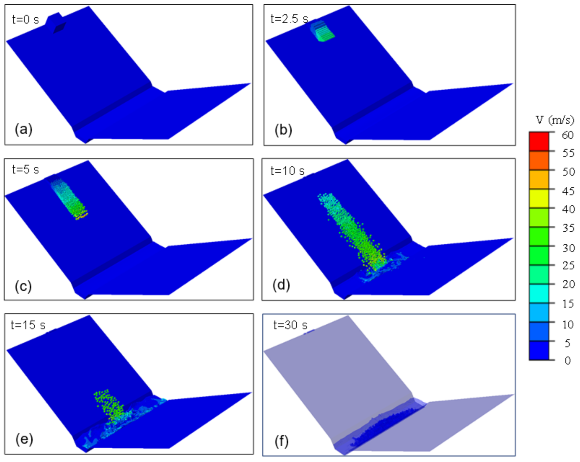
5.1. Typical Runout Process

The results of the simulation, when the number of potential breakage blocks was 1000, are shown in Figure 8, as an example that reflects the entire process of the rock avalanche river-blocking. Figure 8a shows the initial state of the simulation. Then, the source rock started to collapse, and the blocks belonging to the front and upper part represent those prior to collapsing (Figure 8b). After 5 s, the source rock almost completely collapsed into discrete blocks, and all cohesive elements were broken (Figure 8c). Then, the blocks spread and moved along the slope. They were constantly accelerating, and the maximum velocity reached 60 m/s in this period. Upon reaching the river, an impulse wave was created, while the velocity of blocks decreased and ranged from 25 m/s to 45 m/s (Figure 8d). The blocks running out into the river constantly induced impulse waves that spread around, running up the opposite slope (Figure 8e). Once the blocks reached the bottom of the river, they would rapidly slow down, due to friction and collision with the riverbed, and would pile along the riverway. Finally, the impulse wave gradually calmed down, and a landslide dam was formed (Figure 8f).

5.2. Effect of the Fracturing Degree of the Source Rock on Sliding Behavior

In this section, the authors analyzed how the fracturing degree of the source rock affected the sliding process. Figure 9 shows the runout scenes of different fracturing degrees of source rock in the simulation time of 5 s, 7.5 s, and 10 s. The source rock was completely broken during the sliding process, which mean that the higher the fracturing degree of the source rock, the higher the breakage degree of the sliding mass. As the breakage degree of the sliding mass increased, the length and width of the sliding mass generally increased, while the thickness of the sliding mass generally decreased. Regarding the speed, the authors introduced the overall feature speed ( υ ¯ ) to express the magnitude of the mass movement velocity under different fracturing degree conditions. υ ¯ can be defined as follows:
υ ¯   =   2 E k m t
where, E k is the total kinetic energy of the block system, and m t is the total mass of blocks.
Figure 10a,b show the variations of kinetic energy and the overall feature speed ( υ ¯ ) of the block system during the whole process of the rock avalanche river-blocking. Based on the obtained curves, three stages of mass movement were identified: Stage I represented the period when the blocks were moving along the slope before reaching the river, ass discussed in this section; Stage II represented the period from the blocks reaching the river to their complete deposition; Stage III represented the period after the blocks had been completely deposited. Provided that the number of blocks was equal to 1, the sliding mass showed the characteristics of solid motion. Provided that the number of blocks was equal to 8, the interactions between the blocks were very weak, thus the sliding mass still had the characteristics of solid motion. The υ ¯ of the sliding masses under the abovementioned conditions was obviously lower than under other conditions during the sliding process (0–7.5 s), but they had a higher maximum υ ¯ in the whole simulation process when compared to other conditions. This was because under other conditions (i.e., when the number of blocks was 125, 1000, 3375 and 8000), the front of the sliding mass would halt the movement of the rear part when running into water. For other conditions, when the number of blocks was greater than 125, it was evident that, with the increase of the breakage degree of the sliding mass, the υ ¯ of the sliding mass increased. In particular, the difference in υ ¯ under different breakage degree conditions would become more obvious over time. It was observed that the υ ¯ for the condition when the number of blocks was equal to 125 started to be lower than for the other three conditions at the simulation time equal to 1 s. As time passed, the υ ¯ for the conditions when the number of blocks was equal to 1000, or equal to 3375, started being lower than for the condition with more blocks at 4 s and 7 s, respectively. At the end of Stage I, the sliding mass with different breakage degree conditions showed obvious speed differences (Figure 10b). It was evident that the differences in speed of the sliding mass under different breakage degree conditions showed a certain regularity.
The authors concluded that the reason for the above-mentioned phenomenon was related to the structural variation of the sliding mass during the sliding process. After the start of the mass movement, the rock body perpendicular to the direction of sliding had many layers initially (Figure 11a). Due to the gravity and movement of the lower layers of the block, the upper layers of the block were in an extremely unbalanced state, due to which the top and front blocks collapsed, while the central blocks were inserted into the lower blocks. After moving for some time, the number of block layers decreased, and the insertion of the blocks became the main factor in stabilizing the sliding mass structure (Figure 11b). The insertion of the blocks increased the length and width of the sliding mass; the front blocks accelerated, while the rear blocks slowed down to some extent. From a macroscopic point of view, the insertion of the blocks increased the speed of the front landslide body, and decreased the speed of the rear landslide body, when compared to the condition without insertion. The more layers of the block (i.e., higher breakage degree), the more times the front blocks were inserted and accelerated, gaining greater speed. Finally, when only one block layer was present, the sliding mass had a relatively stable structure (Figure 11c). In this paper, the authors refer to this process, of the structure of the sliding mass gradually stabilizing over time, as structure stabilization.
It was evident that the process of mass movement was also a process of structure stabilization. The characteristics of the speed distribution of the sliding mass, with front part accelerating and rear part decelerating, were in accordance with the physical model [45], and this was considered to be one of the reasons that influenced the runout distance. In addition, the process of structure stabilization was also the process of reducing the center of the sliding mass. After the mass movement started, the sliding mass would constantly expand, due to the structure stabilization. According to the contact surface between the sliding mass and the sliding surface (Figure 12), it could be determined that the sliding mass of 125 blocks, representing a low breakage degree, would quickly reach a structurally stable state, where there was only one layer of blocks. After reaching a structurally stable state, the contact area between the sliding mass and the slip surface would change dynamically over time, due to the rotation of the blocks. The contact area would constantly increase in other conditions, but the extent of the variation was different. As time passed, the contact area when the number of blocks was equal to 1000 started to be obviously smaller than for the other two conditions at 4.1 s, while the contact area when the number of blocks was equal to 3375 started to be obviously smaller than for the number of blocks equal to 8000 at 6 s. The variation differences of the contact area with different breakage degree conditions were similar to the variation differences of the mass speed over time (Figure 10b). The higher the breakage degree of the sliding mass, the larger the contact area between the sliding mass and the slip surface, which led to the lower center of the sliding mass. This meant that the sliding mass with higher breakage degree had more gravitational potential energy converted to kinetic energy (Figure 10a), the amount of which was greater than the energy generated by friction due to the larger contact area (Figure 13), thus leading to greater movement speed. According to Figure 10b, it is worth noting that only when the runout distance reached a certain length did the speed difference, caused by the breakage degree, become obvious. When the giant rock slide had enough space to move, the source rock was sufficiently fragmentated, and its structure was sufficiently stabilized, which led to additional mass movement speed. The extra speed of the sliding mass promoted the extra runout distance. This law, that the mass movement speed and the runout distance promoted each other, could be one of the reasons why giant rock avalanches have incredible runout distance and speed in deep valley areas (e.g., the Tibetan Plateau) [3,6].
For a rock avalanche with a very fragmented source and sliding body, and with enough runout distance, the process of structure stabilization can adequately proceed. Therefore, this type of rock avalanche usually exhibits a very low coefficient of flow friction and a large deposition area, such as the Pusa landslide [15] and the Shiaolin landslide [16]. In addition, previous studies have shown that landslides of larger volume usually show a lower flow friction coefficient in the entire sliding process [10,11,12,46]. One reason could be that large-volume landslides have higher gravitational potential energy that can be converted into kinetic energy over long runout distances. From the above-mentioned research, the authors conclude that the process of structure stabilization is important in enhancing the mass movement, and that the factors of high fracturing degree of the source rock, enough runout space, and large source volume will lead to additional mass movement speed and runout distance.

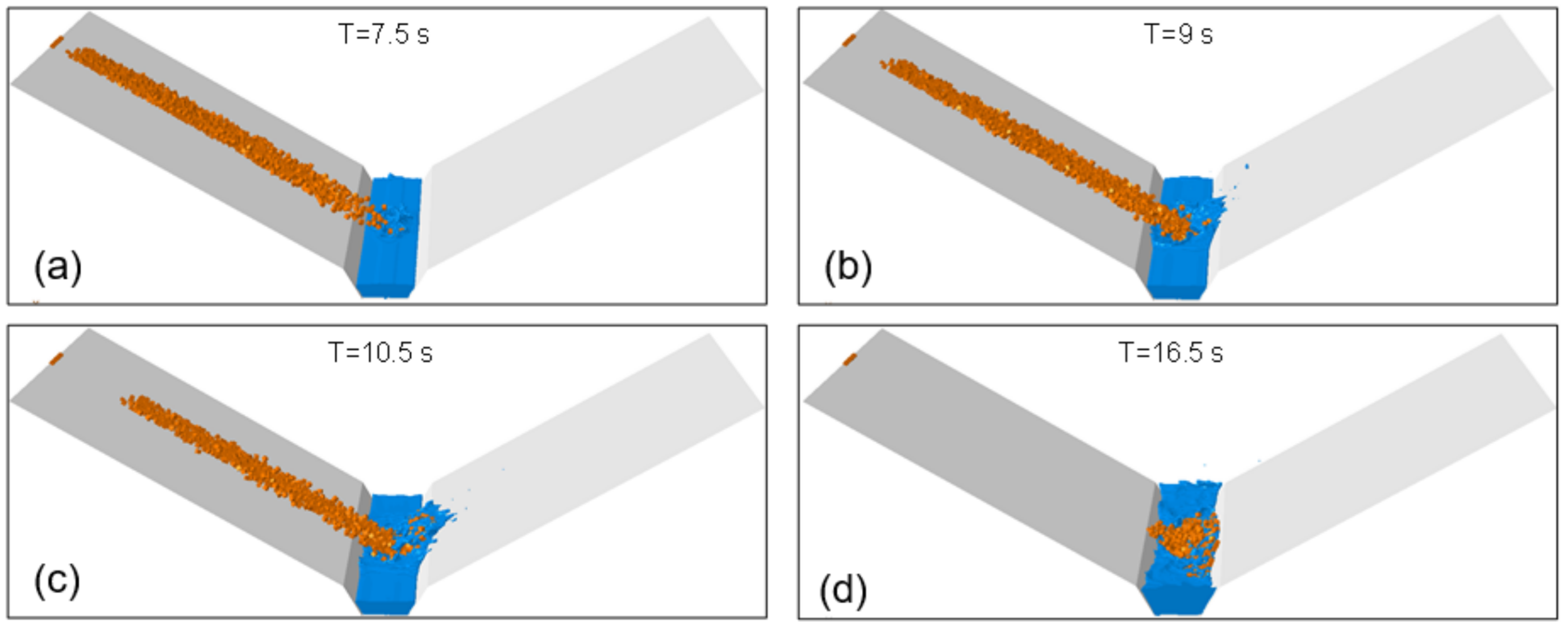
5.3. Effect of the Fracturing Degree of the Source Rock on Impulse Wave Behavior

According to a typical runout process, the impulse wave is generated in 7.5 s, and the maximum height is reached in 10–13 s. Figure 14 shows the variation of the kinetic energy of the river water in the whole simulation process, and Figure 15 shows a typical process of the impulse wave movement with the number of blocks equal to 1000. It can be seen that within 1 s after the sliding mass began running into the water, the kinetic energy of the water would increase rapidly and reach the peak value, then gradually decrease over time. Under conditions that blocked numbers equal to 1 and 8, the kinetic energy of the water would decrease rapidly after reaching the peak value, while the kinetic energy of the water would gradually decrease in other conditions due to the sliding mass constantly running into the water. The peak kinetic energy of the water was highest under the condition of 1 block, then the condition of 8 blocks, and then the condition of 125 blocks. The authors conclude that the reason for this phenomenon was related to the volume of the sliding mass running into the water within the initial 1 s, and that the larger the volume of sliding mass running into the water, the higher the kinetic energy of the water. Under the conditions when the block number equaled 1 and 8, the sliding masses macroscopically did not form a steady flow similar to a fluid, and their movement showed strong discretion. In the case of the same source volume, a larger block generally meant a larger volume of blocks running into the water per unit time. In conditions when the number of blocks was greater than 125, the sliding masses macroscopically formed a steady flow, and their movement showed continuity. Since the volume of the sliding mass running into the water per unit time was approximate, the variation in the kinetic energy of the water showed similarity.
Maximum wave height and velocity of wave propagation are what scholars have been mainly concerned with in previous research. In this study, the authors calculated the maximum height of the impulse waves in the main propagation process (Figure 16a), and their required time to spread to the model boundary (Figure 16b) under different fracturing degree conditions. It was noted that when the block number was equal to 1, the impulse wave had a maximum height of 92 m (which was the maximum height in all conditions), and the time period for the wave to spread to the boundary of the model was shortest with 4.5 s. The impulse wave when the number of blocks was 8 had the second maximum height and the second highest propagation speed in all conditions, followed by the condition when the block number was 125. The maximum heights of the impulse waves in other conditions had similar values, between 20 m and 30 m, and their propagation time to the boundary of the model was generally 9 s, which was obviously longer than for the previous three conditions. It can be seen from Figure 14 and Figure 16 that the maximum energy obtained by the water was generally positively correlated with the maximum height and propagation speed of the impulse waves, which indicated that the kinetic energy obtained by the water would be dissipated in the form of gravitational potential energy and propagation. Therefore, the higher the maximum kinetic energy obtained by the water, the higher the maximum wave height and the higher the propagation speed. The above conclusions illustrate why landslide-induced wave accidents usually occur under the condition of a relatively complete structure of sliding body, such as the Hongyanzi landslide-induced wave accident [18,47] and the Qianjiangping landslide-induced wave accident [17].

5.4. Effect of the Fracturing Degree of the Source Rock on the Formation of the Landslide Dam

Figure 17a,b show the longitudinal profile of landslide dams under different fracturing degrees of the source rock. From the plane view, it was determined that, with the increase of the fracturing degree of the source rock, the shape of the landslide dam tended to stabilize when the number of blocks was larger than 8. From the longitudinal view, a similar phenomenon was observed: that the shape of the landslide dam tended to stabilize when the number of blocks was larger than 125. When the number of blocks was larger than 1000, the shape of the landslide dams varied slightly, and remained almost the same with the increasing of the fracturing degree of the source rock. Previous numerical solutions have proven that the result of the computation will stabilize when the size of the basic elements is smaller than a threshold value, or when the number of basic elements is larger than the threshold value. For example, Masson and Martinez (2000) [48] found that a representative elementary volume (REV) of at least 7–8 particle diameters was sufficient for parameters such as porosity and coordination number, while an REV size of at least 12 particle diameters should be used for the stress tensor. Wiacek, et al. (2012) [49] evaluated the effect of REVs by conducting a uniaxial confined compression test of granular materials, and noted that, provided the volume was approximately five particles or greater in dimension, the computational results were slightly affected. Borykov, et al., [10] (2019) evaluated the sensitivity of DEM simulations to the number of grains, using a dam-break rectangular case with different numbers of particles in a range from 200 to 8000. When the number of grains was greater than 1000, the number of particles did not significantly change the basic behavior of the granular material. In this case, when the size of the blocks was equal to 5 m, their dimension in relation to the river width (the average width was equal to 30 m) could be neglected, and the channel terrain would significantly affect the mass movement behavior. When the size of the blocks was less than 2.5 m, their dimension was small in relation to the width of the river, and the channel terrain would have a relatively small effect on the mass movement behavior, which would result in the stabilization of the landslide dam.

6. Conclusions

In this paper, a series of simulations of rock avalanche river-blocking, based on the CEL method, were used to evaluate the effect of the fracturing degree of the source rock on landslide river-blocking behavior. The simulation of rock avalanche river-blocking showed a common trend and behavior, of sliding mass structure stabilization during runout. Structure stabilization refers to the process in which the number of layers and the center of the sliding mass constantly decrease during sliding. Structure stabilization can provide a lower center of sliding mass with a higher breakage degree of sliding mass, thus achieving higher kinetic energy and speed. In addition to the fracturing degree of the source rock, the authors also concluded that the volume of the sliding mass and the potential runout space affected the mass movement speed. Variations and characteristics of the mass movement speed, contact area, and energy over time also supported the above-mentioned conclusions. The fracturing degree of the source rock greatly affected the behavior of the landslide-induced wave. The volume of the sliding mass running into the river within the first 1 s determined the maximum kinetic energy of the river, with the maximum kinetic energy of the water being large when the structure of the sliding mass was complete. The maximum height and the propagation speed of the impulse wave were positively correlated with the maximum kinetic energy of the water. Regarding the formation of the landslide dams, their shape tended to stabilize with the increase of breakage degree. In addition, the size of the blocks affected the formation of the landslide dams. When the number of blocks was greater than 1000, the shape of the landslide dam would be almost constant with the increase in the number of blocks.
In general, this study evaluated the effect of the fracturing degree of the source rock on river-blocking behavior. We propose a concept of structure stabilization that has a positive significance for the study of rapid long-runout landslides. The application of the CEL method to landslide river-blocking simulation provides experiences for other similar studies, as well as other fluid-solid coupling problems in engineering geology [50]. The triggering factors of landslides, such as rainfall and earthquake, should be further considered in the numerical simulation of a real landslide case.

Author Contributions

Y.B. carried out the numerical simulation and wrote the manuscript. J.C. supervised the overall direction, provided geological data, and helped to revise the manuscript. W.Z. provided funding for the research, and revised the manuscript. Y.L., Z.L. and N.D. supervised the project, and contributed to interpreting the results. All authors have read and agreed to the published version of the manuscript.

Funding

This research was supported by the Second Tibetan Plateau Scientific Expedition and Research Program (STEP) (Grant No. 2021QZKK0202), the Sichuan Science and Technology Program (Grant No. 2021YFS0322), and the Youth Innovation Promotion Association CAS (Grant No. 2019364).

Acknowledgments

We very thank for all the editors and reviewers who have helped us improve and publish the paper.

Conflicts of Interest

The authors declare that they have no conflicts of interest in relation to this work. We declare that we do not have any commercial or associative interest that represents a conflict of interest in connection with the work submitted.

References

  1. Costa, J.E.; Schuster, R.L. The formation and failure of natural dams. Geol. Soc. Am. Bull. 1988, 100, 1054–1068. [Google Scholar] [CrossRef]
  2. Chen, J.; Zhou, W.; Cui, Z.; Li, W.; Wu, S.; Ma, J. Formation process of a large paleolandslide-dammed lake at Xuelongnang in the upper Jinsha River, SE Tibetan Plateau: Constraints from OSL and 14C dating. Landslides 2018, 15, 2399–2412. [Google Scholar] [CrossRef]
  3. Bao, Y.; Shai, S.; Chen, J.; Xu, P.; Sun, X.; Zhan, J.; Zhang, W.; Zhou, X. The evolution of the Samaoding paleolandslide river blocking event at the upstream reaches of the Jinsha River, Tibetan Plateau. Geomorphology 2020, 351, 106970. [Google Scholar] [CrossRef]
  4. Zhang, W.; Wang, J.; Chen, J.; Soltanian, M.R.; Dai, Z.; WoldeGabriel, G. Mass-wasting-inferred dramatic variability of 130,000-year Indian summer monsoon intensity from deposits in the Southeast Tibetan Plateau. Geophys. Res. Lett. 2022, 49, e2021GL097301. [Google Scholar] [CrossRef]
  5. Chigira, M.; Wu, X.; Inokuchi, T.; Wang, G. Landslides induced by the 2008 Wenchuan earthquake, Sichuan, China. Geomorphology 2010, 118, 225–238. [Google Scholar] [CrossRef]
  6. Delaney, K.B.; Evans, S.G. The 2000 Yigong landslide (Tibetan Plateau), rockslide-dammed lake and outburst flood: Review, remote sensing analysis, and process modelling. Geomorphology 2015, 246, 377–393. [Google Scholar] [CrossRef]
  7. Liu, W.; Ju, N.; Zhang, Z.; Chen, Z.; He, S. Simulating the process of the Jinshajiang landslide-caused disaster chain in October 2018. Bull. Eng. Geol. Environ. 2020, 79, 2189–2199. [Google Scholar] [CrossRef]
  8. Hungr, O.; Evans, S.G. Entrainment of debris in rock avalanches: An analysis of a long runout mechanism. Geol. Soc. Am. Bull. 2004, 116, 1240–1252. [Google Scholar] [CrossRef]
  9. Bao, Y.; Han, X.; Chen, J.; Zhang, W.; Zhan, J.; Sun, X.; Chen, M. Numerical assessment of failure potential of a large mine waste dump in Panzhihua City, China. Eng. Geol. 2019, 253, 171–183. [Google Scholar] [CrossRef]
  10. Borykov, T.; Mège, D.; Mangeney, A.; Richard, R.; Gurgurewicz, J.; Lucas, A. Empirical investigation of friction weakening of ter-restrial and Martian landslides using discrete element models. Landslides 2019, 16, 1121–1140. [Google Scholar] [CrossRef] [Green Version]
  11. Heim, A. Bergsturz und Menschenleben (Landslides and Human Lives); Skermer, N., Translator; Bitech Press: Vancouver, BC, Canada, 1932. [Google Scholar]
  12. Staron, L.; Lajeunesse, E. Understanding how volume affects the mobility of dry debris flows. Geophys. Res. Lett. 2009, 36, 91–100. [Google Scholar] [CrossRef] [Green Version]
  13. Aaron, J.; McDougall, S. Rock avalanche mobility: The role of path material. Eng. Geol. 2019, 257, 105–126. [Google Scholar] [CrossRef]
  14. Ibañez, J.; Hatzor, Y. Rapid sliding and friction degradation: Lessons from the catastrophic Vajont landslide. Eng. Geol. 2018, 244, 96–106. [Google Scholar] [CrossRef]
  15. Fan, X.; Yang, F.; Siva Subramanian, S.; Xu, Q.; Feng, Z.; Mavrouli, O.; Peng, M.; Ouyang, C.; Jansen, J.D.; Huang, R. Prediction of a multi-hazard chain by an integrated numerical simulation approach: The Baige landslide, Jinsha River, China. Landslides 2020, 17, 147–164. [Google Scholar] [CrossRef]
  16. Tsou, C.; Feng, Z.; Chigira, M. Catastrophic landslide induced by Typhoon Morakot, Shiaolin, Taiwan. Geomorphology 2010, 127, 166–178. [Google Scholar] [CrossRef] [Green Version]
  17. Yin, Y.; Huang, B.; Chen, X.; Liu, G.; Wang, S. Numerical analysis on wave generated by the Qianjiangping landslide in Three Gorges Reservoir, China. Landslides 2015, 12, 355–364. [Google Scholar] [CrossRef]
  18. Zhou, J.; Xu, F.; Yang, X.; Yang, Y.; Lu, P. Comprehensive analyses of the initiation and landslide-generated wave processes of the 24 June 2015 Hongyanzi landslide at the Three Gorges Reservoir, China. Landslides 2016, 13, 589–601. [Google Scholar] [CrossRef]
  19. Bowman, E.T.; Take, W.A.; Rait, K.L.; Hann, C. Physical models of rock avalanche spreading behaviour with dynamic frag-mentation. Can. Geotech. J. 2012, 49, 460–476. [Google Scholar] [CrossRef] [Green Version]
  20. Liao, H.; Yang, X.; Lu, G.; Tao, J.; Zhou, J. Experimental study on the formation of landslide dams by fragmentary materials from successive rock slides. Bull. Eng. Geol. Environ. 2020, 79, 1591–1604. [Google Scholar] [CrossRef]
  21. Bisantino, T.; Fischer, P.; Gentile, F. Rheological characteristics of debris-flow material in South-Gargano watersheds. Nat. Hazards 2009, 54, 209–223. [Google Scholar] [CrossRef]
  22. Pellegrino, A.M.; Anna, S.D.S.; Schippa, L. An integrated procedure to evaluate rheological parameters to model debris flows. Eng. Geol. 2015, 196, 88–98. [Google Scholar] [CrossRef]
  23. Kaczmarek, Ł.; Popielski, P. Selected components of geological structures and numerical modeling of slope stability. Open Geosci. 2019, 11, 208–218. [Google Scholar] [CrossRef]
  24. Lin, C.; Lin, M. Evolution of the large landslide induced by Typhoon Morakot: A case study in the Butangbunasi River, southern Taiwan using the discrete element method. Eng. Geol. 2015, 197, 172–187. [Google Scholar] [CrossRef]
  25. Lo, C.; Lin, M.; Tang, C.; Hu, C. A kinematic model of the Hsiaolin landslide calibrated to the morphology of the landslide deposit. Eng. Geol. 2011, 123, 22–39. [Google Scholar] [CrossRef]
  26. Chen, K.; Wu, J. Simulating the failure process of the Xinmo landslide using discontinuous deformation analysis. Eng. Geol. 2018, 239, 269–281. [Google Scholar] [CrossRef]
  27. Do, T.; Wu, J. Simulating a mining-triggered rock avalanche using DDA: A case study in Nattai North, Australia. Eng. Geol. 2020, 264, 105386. [Google Scholar] [CrossRef]
  28. Sosio, R.; Crosta, G.B.; Hungr, O. Complete dynamic modeling calibration for the Thurwieser rock avalanche (Italian central alps). Eng. Geol. 2008, 100, 11–26. [Google Scholar] [CrossRef]
  29. Pastor, M.; Blanc, T.; Haddad, B.; Petrone, S.; Sanchez Morles, M.; Drempetic, V.; Issler, D.; Crosta, G.B.; Cascini, L.; Sorbino, G.; et al. Application of a SPH depth-integrated model to landslide run-out analysis. Landslides 2014, 11, 731–812. [Google Scholar] [CrossRef] [Green Version]
  30. Llano-Serna, M.A.; Farias, M.M.; Pedroso, D.M. An assessment of the material point method for modelling large scale runout processes in landslides. Landslides 2016, 13, 1057–1066. [Google Scholar] [CrossRef]
  31. Ouyang, C.; An, H.; Zhou, S.; Wang, Z.; Su, P.; Wang, D.; Cheng, D.; She, J. Insights from the failure and dynamic characteristics of two sequential landslides at Baige village along the Jinsha River, China. Landslides 2019, 16, 1397–1414. [Google Scholar] [CrossRef]
  32. Scaringi, G.; Fan, X.; Xu, Q.; Liu, C.; Ouyang, C.; Domènech, G.; Yang, F.; Dai, L. Some considerations on the use of numerical methods to simulate past landslides and possible new failures: The case of the recent Xinmo landslide (Sichuan, China). Landslides 2018, 15, 1359–1375. [Google Scholar]
  33. Huang, Y.; Zhu, C. Simulation of flow slides in municipal solid waste dumps using a modified MPS method. Nat. Hazards 2014, 74, 491–508. [Google Scholar] [CrossRef]
  34. Zhu, C.; Chen, Z.; Huang, Y. Coupled moving particle simulation-finite-element method analysis of fluid-structure interaction in geodisasters. Int. J. Geomech. 2021, 21, 04021081. [Google Scholar] [CrossRef]
  35. Jeong, S.; Lee, K. Analysis of the impact force of debris flows on a check dam by using a coupled Eulerian-Lagrangian (CEL) method. Comput. Geotech. 2019, 116, 103214. [Google Scholar] [CrossRef]
  36. Koshizuka, S.; Oka, Y.; Tamako, H. A Particle Method for Calculating Splashing of Incompressible Viscous Fluid; American Nuclear Society, Inc.: La Grange Park, IL, USA, 1995. [Google Scholar]
  37. Tan, H.; Chen, S. A hybrid DEM-SPH model for deformable landslide and its generated surge waves. Adv. Water Resour. 2017, 108, 256–276. [Google Scholar] [CrossRef]
  38. Zhang, W.; Lan, Z.; Ma, Z.; Tan, C.; Que, J.; Wang, F.; Cao, C. Determination of statistical discontinuity persistence for a rock mass characterized by non-persistent fractures. Int. J. Rock Mech. Min. Sci. 2020, 126, 104177. [Google Scholar] [CrossRef]
  39. Xi, X.; Yang, S.; McDermott, C.; Shipton, Z.; Fraser-Harris, A.; Edlmann, K. Modelling rock fracture induced by hydraulic pulses. Rock Mech. Rock Eng. 2021, 54, 3977–3994. [Google Scholar] [CrossRef]
  40. Ma, G.; Zhou, W.; Ng, T.; Cheng, Y.; Chang, X. Microscopic modeling of the creep behavior of rockfills with a delayed particle breakage model. Acta Geotech. 2015, 10, 481–496. [Google Scholar] [CrossRef]
  41. Ditoro, G.; David, L.G.; Terry, E.T. Friction falls towards zero in quartz rock as slip velocity approaches seismic rates. Nature 2004, 427, 436–439. [Google Scholar] [CrossRef]
  42. Han, R.; Shimamoto, T.; Hirose, T.; Ree, J.; Ando, J. Ultralow friction of carbonate faults caused by thermal decomposition. Science 2007, 316, 878–881. [Google Scholar] [CrossRef] [Green Version]
  43. McDougall, S. 2014 Canadian Geotechnical Colloquium: Landslide runout analysis—Current practice and challenges. Can. Geotech. J. 2017, 54, 605–620. [Google Scholar] [CrossRef] [Green Version]
  44. Hu, W.; Huang, R.; McSaveney, M.; Yao, L.; Xu, Q.; Feng, M.; Zhang, X. Superheated steam, hot CO2 and dynamic recrys-tallization from frictional heat jointly lubricated a giant landslide: Field and experimental evidence. Earth Planet. Sci. Lett. 2019, 510, 85–93. [Google Scholar] [CrossRef]
  45. Davies, T.R.; McSaveney, M.J. Runout of dry granular avalanches. Can. Geotech. J. 1999, 36, 313–320. [Google Scholar] [CrossRef]
  46. Johnson, B.C.; Campbell, C.S. Drop height and volume control the mobility of long-runout landslides on the Earth and Mars. Geophys. Res. Lett. 2017, 44, 12091–12097. [Google Scholar] [CrossRef] [Green Version]
  47. Huang, B.; Yin, Y.; Du, C. Risk management study on impulse waves generated by Hongyanzi landslide in Three Gorges Reservoir of China on June 24, 2015. Landslides 2016, 13, 603–616. [Google Scholar] [CrossRef]
  48. Masson, S.; Martinez, J. Effect of particle mechanical properties on silo flow and stresses from distinct element simulations. Powder Technol. 2000, 109, 164–178. [Google Scholar] [CrossRef]
  49. Wiacek, J.; Molenda, M.; Ooi, J.Y.; Favier, J.F. Experimental and numerical determination of representative elementary volume for granular plant materials. Granul. Matter 2012, 14, 449–456. [Google Scholar] [CrossRef] [Green Version]
  50. Zhang, X.D.; Ye, P.; Wu, Y.J.; Zhai, E.C. Experimental study on simultaneous heat-water-salt migration of bare soil subjected to evaporation. J. Hydrol. 2022, 609, 127710. [Google Scholar] [CrossRef]
Figure 1. A typical case of different fracturing degrees of source rock on the upstream reaches of the Jinsha River: (a) low fracturing degree of source rock; (b) medium fracturing degree of source rock; and (c) high fracturing degree of source rock.
Minerals 12 00901 g001
Figure 2. Sketch of: (a) Lagrangian Mesh; and (b) Eulerian Mesh.
Minerals 12 00901 g002
Figure 3. Principles of the CEL contact. (a) CEL Sketch; and (b) data transfer on the coupling interface.
Minerals 12 00901 g003
Figure 4. Geometry of the water collapse simulation: (a) plane dimension of the model; (b) boundary conditions of the three-dimension model.
Minerals 12 00901 g004
Figure 5. The process of water column collapse. Left column: the experiment. Middle column: SPH results. Right column: CEL results obtained in this study.
Minerals 12 00901 g005
Figure 6. Geometry of the landslide river-blocking model: (a) longitudinal profile view; (b) plane view.
Minerals 12 00901 g006
Figure 7. Six conditions of different fracturing degrees of a source rock: (a) structural plane number: 0; (b) structural plane number: 1 × 1 × 1 in each dimension; (c) structural plane number: 4 × 4 × 4 in each dimension; (d) structural plane number: 9 × 9 × 9 in each dimension; (e) structural plane number: 14 × 14 × 14 in each dimension; (f) structural plane number: 19 × 19 × 19 in each dimension.
Minerals 12 00901 g007
Figure 8. The whole process of rock avalanche river-blocking, based on the contour velocity map: (a) initial state of the model; (b) rock blocks collapse; (c) runout behavior; (d) sliding mass reaching the river; (e) induced wave behavior; (f) formation of a landslide dam.
Minerals 12 00901 g008
Figure 9. Scenes of the runout behavior for different fracturing degrees of the source rock.
Minerals 12 00901 g009aMinerals 12 00901 g009b
Figure 10. (a) Total kinetic energy of the computation domain, and (b) the overall feature speed over time. t1, t2 and t3 represent the time when the number of blocks equal to 125, 1000, and 3375 begin to show an obvious difference in movement speed, in relation to the higher breakage degree of the sliding mass.
Minerals 12 00901 g010
Figure 11. The process of stabilization of sliding mass structure during mass movement. (a) initial failure state; (b) dynamic sliding process (c) final stable state.
Minerals 12 00901 g011
Figure 12. Contact area between blocks and slip surface from 0 s to 8 s under conditions of 125, 1000, 3375, and 8000 blocks. t1, t2 and t3 represent the time when the lowest breakage degree of sliding mass begins to have an obvious difference in the contact area from the sliding mass with higher breakage degree.
Minerals 12 00901 g012
Figure 13. Energy generated by friction from 0 s to 8 s under conditions of 125, 1000, 3375, and 8000 blocks.
Minerals 12 00901 g013
Figure 14. Kinetic energy of river water over time.
Minerals 12 00901 g014
Figure 15. The propagation process of the impulse wave: (a) initial status; (b) development process; (c) maximum height; (d) dissipation process.
Minerals 12 00901 g015
Figure 16. The characteristics of impulse waves under different fracturing conditions. N represents the potential number of blocks in the model, and: (a) the maximum height over time; (b) impulse waves propagation time to the boundary of the model.
Minerals 12 00901 g016
Figure 17. The shape of the landslide dam under different fracturing degree conditions: (a) plane view of landslide dam; (b) longitudinal profile of landslide dam.
Minerals 12 00901 g017
Table 1. Numerical parameters of the water collapse simulation.
MaterialParameters
Water ρ (kg/m3) c 0 (m/s) s Γ 0 η (Pa·s)
10001500000.001
Glass tank ρ (kg/m3)E (MPa) ν f/
180078,5000.30.001
ρ : density of material; c 0 : reference sound speed; s : slope of Us-Up curve; Γ 0 : Material constant; η : viscosity; E: Young’s modules; ν : Poisson’s ratio; and f: friction coefficient.
Publisher’s Note: MDPI stays neutral with regard to jurisdictional claims in published maps and institutional affiliations.

