Automated Quantitative Mineralogy Optimized for Simultaneous Detection of (Precious/Critical) Rare Metals and Base Metals in A Production-Focused Environment

Abstract

Automated Scanning Electron Microscopy (ASEM) systems are applied in the mining industry to quantify the mineralogy of the ore feed and products. With society pushing towards sustainable mining, this quantification should be comprehensive and include trace minerals since they are often either deleterious or potential by-products. Systems like QEMSCAN^® offer a mode for trace mineral analysis (TMS mode); However, it is unsuitable when all phases require analysis. Here, we investigate the potential of detecting micron-sized trace minerals in fieldscan mode using the QEMSCAN^® system with analytical settings in line with the mining industry. For quality comparison, analysis was performed at a mining company and a research institution. This novel approach was done in full collaboration with both parties. Results show that the resolution of trace minerals at or below the scan resolution is difficult and not always reliable due to mixed X-ray signals. However, by modification of the species identification protocol (SIP), quantification is achievable, although verification by SEM-EDS is recommended. As an add-on to routine quantitative analysis focused on major ore minerals, this method can produce quantitative data and information on mineral association for trace minerals of precious and critical metals which may be potential by-products in a mining operation.

1. Introduction

As the need for sustainability in mining is becoming increasingly important amongst the public, decision makers and the industry itself, detailed investigations into what ore deposits actually contain in terms of various minerals, potential by-products and industrial minerals are needed. By making use of a larger proportion of the mined ore (recovering also the trace metals) mining operations can be more sustainable and this will potentially also be beneficial in gaining public acceptance for mining (social license to operate). Precious metals such as Au and Ag are already readily produced as main- or by-products in many mining ventures even if they occur only in trace amounts and numerous metals could potentially follow the precious metals as by-products in a number of mining operations worldwide. Many European ore deposits contain various amounts of trace metals classified as “Critical Raw Material” (CRM) by the European Commission, i.e., they are of high economic importance for the EU but with a high risk associated with their supply [1].

While trace metal production may not be economically profitable at the moment this could change in the future as metal prices increase and the pressure is increasing for more sustainable mining. Hence, for sustainability as well as economic reasons, the trace mineral and metal characterization of an ore deposit should be considered when planning for a mining operation, and also in operating mines.

In order to predict trace metal deportment during processing of the ore, a good understanding of their mineralogical and textural characterization is necessary. Due to their low abundance in ore deposits and often fine-grained (<50 µm) nature, identification and quantification of trace minerals is difficult and requires the use of advanced micro-analytical techniques. Many capable techniques were developed over the last few decades, each with its own advantages and disadvantages [2], but especially, Automated Scanning Electron Microscopy (ASEM) systems found wide-spread acceptance and application in the mining industry. These systems provide fast and reliable quantification of the mineralogy and textures in a sample. Most prominent are the Quantitative Evaluation of Mineralogy by a SCANning electron microscope (QEMSCAN^®) system and the Mineral Liberation Analyzer (MLA) system [3,4].

The QEMSCAN^® system is the third generation of automated mineral analysis systems based on the then-named QEM*SEM^® system. QEM*SEM^®, was developed at the request of the mining industry by the Commonwealth Scientific and Industrial Research Organization (CSIRO) in Australia in the 1970s and marked the first automated mineral analyzer [5,6]. The MLA system is based on the concepts of Hall [7] and became commercially available in 2000 through FEI Company and JKTech, whilst QEMSCAN^® was marketed by Intellection Pty Ltd. Both systems, QEMSCAN^® and MLA, utilize backscattered electrons (BSE) and energy dispersive X-ray spectra (EDS) to create digital mineral images. In the QEMSCAN^® system, low-count X-ray mapping is preferentially used for mineral classification. This is done by comparison of the X-ray element-spectra to existing mineral databases. BSE brightness is used to distinguish particles from the mounting media. A summary of the QEMSCAN^® system and its various application modes is provided by Gottlieb et al. [3], Goodall et al. [8], and Pirrie and Rollinson [9]. By contrast, in the MLA system, particles are often defined through the BSE brightness and subsequently classified by one X-ray spectrum per particle. For particles of similar BSE brightness, X-ray mapping is used. The MLA system is described in detail by Gu [4]. While both systems are still widely applied in the industry and by research institutions, their commercial production has currently been terminated. This has given rise to new ASEM systems, most prominently the ZEISS Mineralogic Mining system and the TESCAN Integrated Mineral Analyzer (TIMA) [10]. These systems come with some improvements, such as faster speed of analysis. An introduction to the ZEISS Mineralogic Mining system is provided by Graham et al. [11] and references therein, and the principles and applications of the TIMA system are described by Hrstka et al. [10].

In the mining industry, ASEM systems are mostly applied for routine scans of particulate samples of ore and tailings concentrate to identify and quantify the mineralogy of the ore feed and products. Instruments are typically calibrated for fast acquisition rates to enable a high sample throughput. This comes at the expense of precision and resolution. As a consequence, trace minerals are often undetected due to their grain size being at or below the scan resolution. Most ASEM systems provide an analytical mode targeted towards the analysis of trace minerals (such as TMS mode for QEMSCAN^®) and its usefulness for characterization of, e.g., Au has been demonstrated [8,12,13,14]. However, this analytical mode hardly finds application for deposits where trace minerals are only by-products, or of no current economic interest. Furthermore, since the TMS mode utilizes a BSE brightness threshold to filter for trace minerals, it is hardly applicable if the sample is enriched in Pb- and Bi-minerals due to their similar BSE brightness compared to Au-minerals. This forces the system to analyze many more particles than necessary (so-called false particles) and is thus more time-consuming. Hence, there is a need to improve detection of trace phases in general analyses.

Here, we compare results of analysis of a polished thin section from a Cu-(W-Au) ore between two QEMSCAN^® systems; one is an industry-system (Boliden AB), the other a research-system (Camborne School of Mines). For the research-oriented scan, the setup of the analysis was thoroughly planned and much time was spent on the post-processing of the raw data, so this scan is assumed to be of the highest quality and used as a measure for the relative quality of the routine industrial scan. The goal was to determine the overall quality of general routine industrial scans and the possibility of detecting and quantifying trace phases at or below the scan resolution. Ideally, a scan should provide a basic idea of trace mineral mineralization in a sample and help the operator/decision maker decide if more detailed analysis is worth pursuing. In this case, the trace mineral Au was used to find an optimum methodology for detecting and quantifying trace minerals but the methodology presented applies to all trace minerals in an ore body. A guide towards analysis is provided. This analysis is novel in its collaborative inter-lab comparison between the industry and a scientific institution.

2. Materials and Methods

To promote analysis of uncrushed rock samples by ASEM systems prior to processing, a thin section sample of a drill core was chosen instead of a particulate sample for this analysis, despite the more common usage of particulate samples in the mining industry. Uncrushed samples have a higher uncertainty of representativeness, but they allow the study of original features like mineral distribution, structures and textures which carry important information for processing of the ore but are partly lost during crushing. Hence, for comprehensive ore characterization to aid in early mine planning, uncrushed rock samples are most suitable. To limit uncertainties, appropriate sampling and sufficient volume are necessary [15], in fact, possibilities to routinely scan drill core pieces are currently tested at Boliden AB. Furthermore, ideally, analysis should be performed on both crushed and uncrushed rock samples.

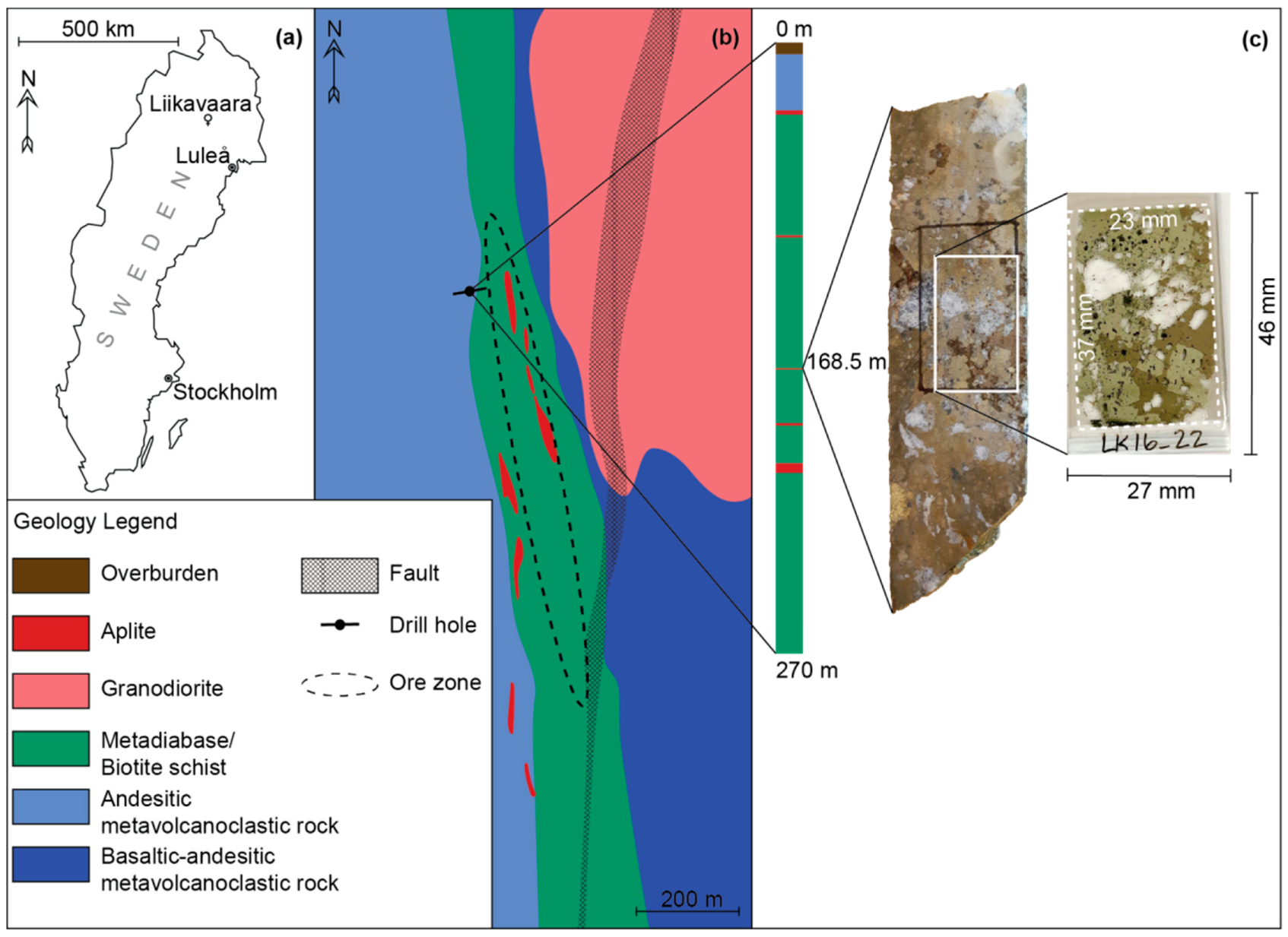
The sample selected was from the Liikavaara Cu-(W-Au) deposit, an intrusion-related vein-style deposit in Northern Sweden (Figure 1a,b), located close to the world-class Aitik Cu-Au deposit where the Liikavaara ore will be processed. Chalcopyrite, pyrite and pyrrhotite constitute the major ore minerals. Sphalerite, galena, scheelite, molybdenite, marcasite and magnetite are minor. The deposit also hosts several trace metals including Au, Ag, Bi and Sn which commonly occur in fine-grained minerals (<20 µm) [16]. The trace metal mineralogy is presented in

Table 1. Trace metal mineralogy of the Liikavaara Cu-(W-Au) deposit.

Trace Metal	Mineralogy
Au	native Au, electrum (Au-Ag-alloy, Ag > 20%)
Ag	hessite (Ag2Te), acanthite (Ag2S), native Au, electrum
Bi	native Bi, pilsenite (Bi4Te3), tetradymite (Bi2Te2S), bismuthinite (Bi2S3)
Sn	cassiterite (SnO2)

, and a detailed description of the geology and mineralogy of the deposit is given by Zweifel [17] and Warlo et al. [16].

The deposit is currently in the pre-production stage, and production is estimated to start in 2023. Copper will be the primary commodity and Au and Ag will be by-products. Production of W, despite its enrichment and classification as a CRM, would require an additional processing step and is thus unprofitable at present. Bismuth is known for its potential to contaminate and lower the quality of the Cu concentrate, thus having good control over its mineralogy and distribution is beneficial.

The pre-production stage of the Liikavaara deposit, its enrichment in several trace metals of interest, a diverse fine-grained mineralogy, and previous studies, make the Liikavaara Cu-(W-Au) deposit an ideal candidate for this type of study.

The selected core sample (mineralized quartz vein from the proximal ore zone) was prepared into a polished thin section of 27 × 46 mm with a sample size of 23 × 37 mm (Figure 1c). In the corresponding other half of the drill core, an Au-grade of ca. 6 ppm was measured over a 1.3 m section.

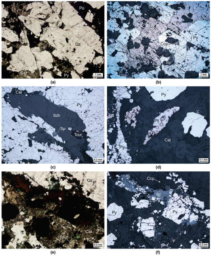
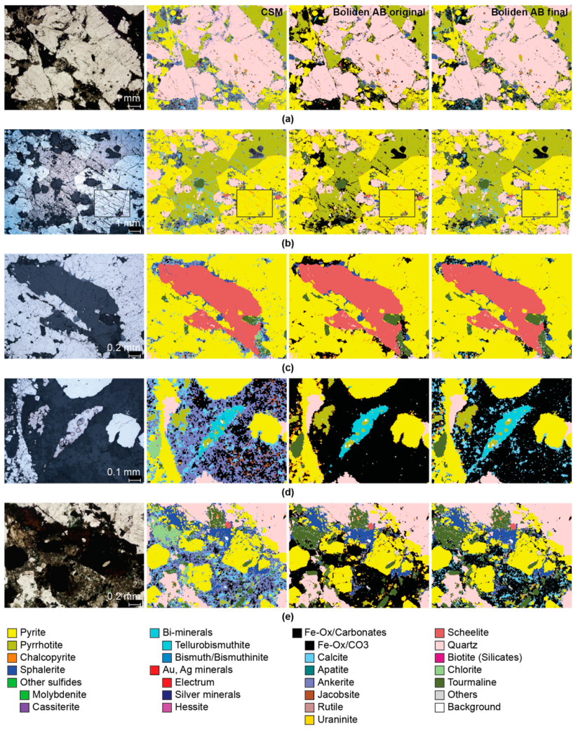
The sampled vein is composed of quartz with minor tourmaline and scattered patches altered by fine-grained (<20 µm) calcite and chlorite (Figure 2a,e). It is strongly mineralized by pyrite and pyrrhotite, and by minor chalcopyrite and sphalerite (Figure 2b,f). Pyrite and pyrrhotite vary in grain sizes from a few microns to several centimeters in width. Grains are often fractured but pyrite retains a subhedral shape (Figure 2b,f). Chalcopyrite and sphalerite exist mostly as crack fillings and along grain boundaries in pyrite and quartz, but are also associated with tourmaline and disseminated (<50 µm) in areas altered by calcite and chlorite (Figure 2b,f). 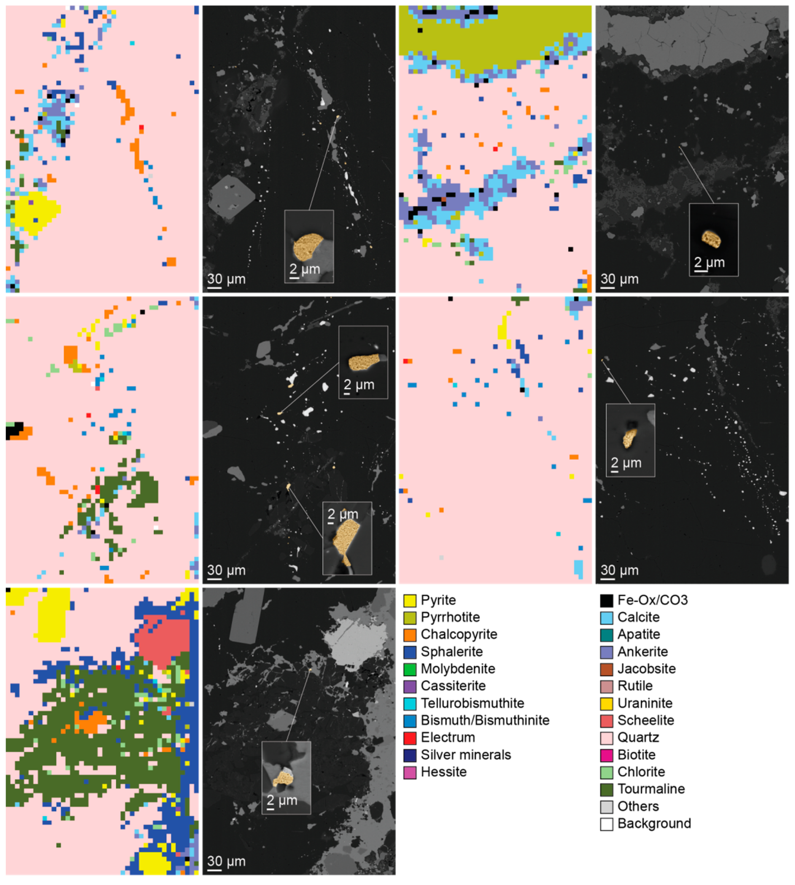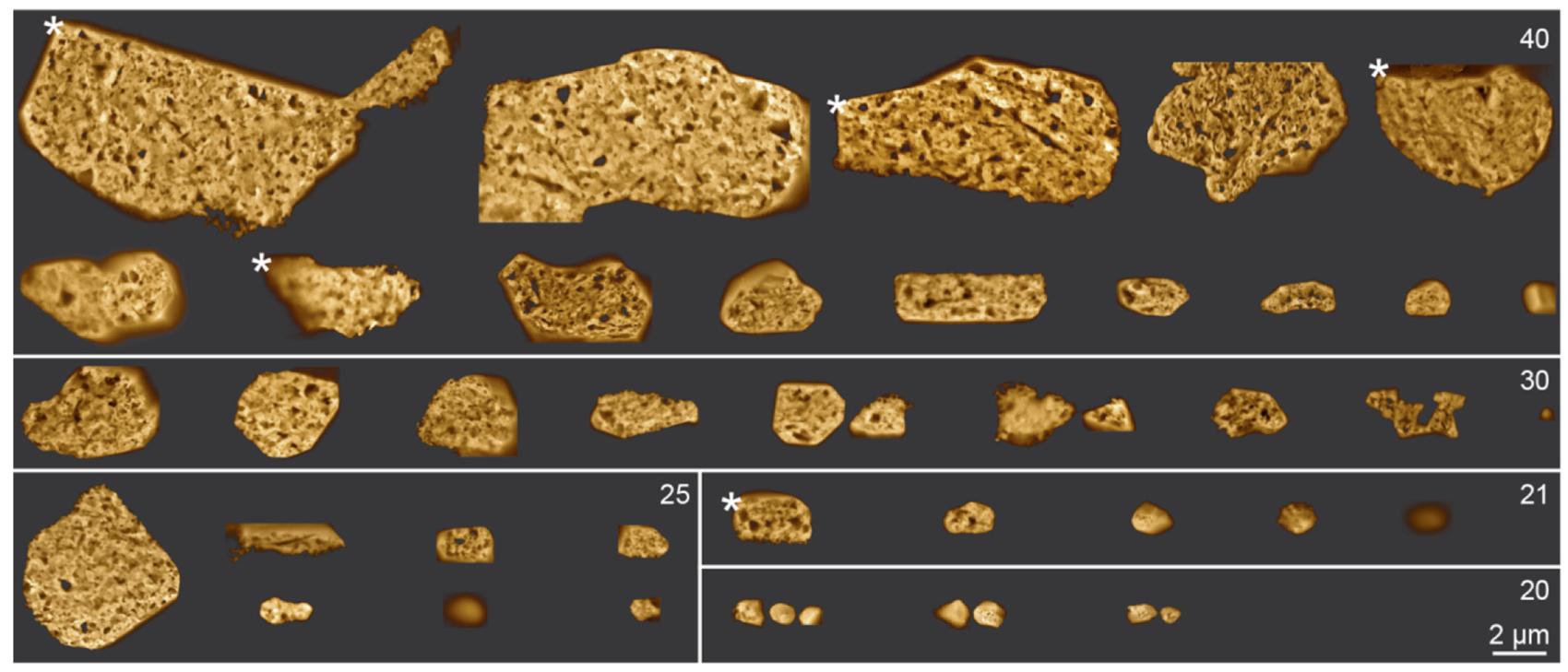Several grains of scheelite (>1 cm), and one 400 µm grain of pilsenite, are observed (Figure 2c–e). SEM-BSE imaging coupled with EDS analysis revealed the occurrence of native bismuth, hessite, bismuthinite and electrum. Grains were mostly below 10 µm in size (Figure 3a–d).

Petrography of the sample prior to QEMSCAN^® analysis was carried out with a petrographic microscope (Nikon ECLIPSE E600 POL) in transmitted and reflected light, and with a scanning electron microscope (Zeiss Merlin FEG-SEM) at Luleå University of Technology. The same SEM was used for verification of the trace minerals detected by the QEMSCAN^® analyses.

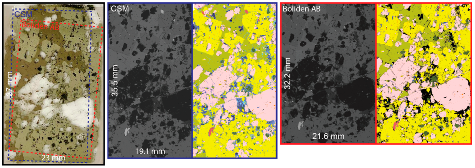
The polished thin section was first analyzed with the QEMSCAN^® system at Camborne School of Mines (CSM), University of Exeter, Penryn, UK, to comprehensively characterize the mineralogy of the sample with emphasis on the detection and identification of trace metal minerals. This consists of a QEMSCAN^® 4300 (Zeiss EVO® 50 SEM with W-filament, four EDS, and an electron backscatter detector) using iMeasure version 4.2 SR1 software for data collection, and iDiscover 4.2SR1 and 4.3 software for data processing. The sample was carbon coated to 25 nm at CSM prior to analysis. The fieldscan measurement mode was performed at an X-ray resolution of 10 µm using a horizontal field width of 1500 µm (150 × 150 analysis points per field), with a measurement area of approximately 19 mm × 35.5 mm (Figure 4), resulting in ~7 million analysis points and a scan time of 10:20 h. The X-ray count per pixel used the default of 1000 counts. For mineral identification, a modified version of the standard LCU5 Species Identification Protocol (SIP) was used, following the guidance in Section 7 of Rollinson et al. [18]. During data processing, particular emphasis was placed on the trace metal minerals to enable identification of these and take into account their small size (some were at the single pixel scale), which results in mixed spectra. This included electrum, bismuth minerals, molybdenite and the silver minerals. However, the SIP (mineral database) was customized to the entire sample, to ensure all the minerals in the sample were identified as accurately as possible, which involved checking all the minerals present and developing the database entries as required. This, for example, involved improving existing entries, adding boundary categories for existing minerals caused by mixed spectra, and adding new entries for the trace metal minerals to ensure they were as accurately captured as possible given their small size.

The same thin section was then measured at Boliden AB, Boliden, Sweden with a similar objective. However, settings were chosen to reflect a routine industrial application. At Boliden AB, a QEMSCAN^® 650 (FEI with W-filament, two EDS, and an electron backscatter detector) was used with iMeasure version 5.4 software for data collection and iDiscover 5.4 software for data processing. The fieldscan measurement mode was performed at an X-ray resolution of 5 µm using a horizontal field width of 1500 µm (300 × 300 analysis points per field), with a measurement area of approximately 21.5 mm × 32 mm (Figure 4), resulting in ~24.6 million analysis points and a scan time of 23:50 h. The X-ray count per pixel used the default of 1000 counts. For mineral identification, a custom SIP for the Aitik deposit, based on several scientific and in-house mineralogical studies, was modified and adapted to the mineralogy of the Liikavaara Cu-(W-Au) deposit. After the measurement, an initial search for unknown phases was performed and corresponding minerals added to the SIP. This was followed by a data processing routine. Comparison of the results with the analysis at CSM led to application of the “boundary phase processor” and to several more additions to the mineral list (especially for Au-phases) to improve data quality (see Section 3).

3. Results

3.1. Results Prior to Optimisation

Results from both QEMSCAN^® analyses, at CSM and Boliden AB, respectively, showed, overall, a good agreement with earlier detailed petrographic and SEM studies; however, there were some key differences between the data sets.

3.1.1. Measured Area

The areas scanned by QEMSCAN^® differed in size between CSM and Boliden AB and did not cover the entire sample (Figure 4). Limitations were set by the design of the sample holders. Furthermore, it was not possible to match the produced BSE and mineral maps of Boliden AB and CSM through image manipulation such as cutting, rotating, and stretching. The reason for this is not certain, but could be an issue with magnification calibration during stitching of the individual fields to a unified image for either operator. These issues prevented full quantitative comparison of the modal mineralogy and mineral association between the two datasets.

3.1.2. BSE Map

Several fields of the BSE map from Boliden AB showed a shift in brightness and contrast to the surrounding fields which was not observed in the CSM map (Figure 5). This potentially indicates a poor vacuum condition in the SEM chamber during measurement, or beam fluctuation; however, no impact on the mineral map was observed.

3.1.3. Mineralogy

The QEMSCAN^® analysis by CSM agreed with the mineralogy described by light optical microscopy and SEM of the selected sample (see Section 2). Major and minor sulfides and silicates were confirmed. Electrum, hessite, and Bi-minerals were all detected (Figure 6 and Figure 7d). Additionally, traces of molybdenite, cassiterite, uraninite and Ag-minerals (other than hessite) were detected. Many of these phases mark single pixels in the mineral map. The fine-grained clusters of calcite observed during petrographic analysis were resolved to be complex intergrowths of calcite, ankerite and Fe-Ox/CO₃ (mostly goethite) (Figure 7d,e). Bi-minerals were categorized into Bi-tellurides and native bismuth/bismuthinite. No differentiation was made between Bi-tellurides (e.g., pilsenite and tetradymite). Similarly, native bismuth and bismuthinite were grouped together due to difficulties in separating Bi and S at the scan resolution in QEMSCAN^® analysis. A total of seven pixels were identified as electrum (Figure 6). Follow-up work with the SEM-EDS confirmed these pixels correlated with six different grains of native Au and electrum in the sample. The grains were typically associated with quartz and often found within areas rich in Bi-minerals. The Au grains ranged in size from 6 × 12 µm to 2 × 3 µm (Figure 6). This means, despite their sub 10 µm grain sizes, a 10 µm resolution scan was sufficient to detect them. Further SEM-EDS studies revealed several more native gold and electrum grains (mostly <5 µm) in the immediate surrounding of the grains detected by the QEMSCAN^® scan. Additionally, sub 5 µm droplet-shaped grains of native bismuth with partitioning of gold were frequently observed [19]. None of the pixels corresponding to these grains were identified as Au-minerals by the QEMSCAN^® analysis of CSM.

Mineralogy was less detailed for the Boliden AB data set. Only 13 phases were distinguished by Boliden AB compared to 23 phases at CSM (which included all 13 phases from Boliden AB) (Figure 7). Minor sulfides were compiled under “other sulfides”. Similarly, silicates were grouped together with the exception of quartz, tourmaline and chlorite. For trace metals, only “Bi-minerals” and “Au, Ag minerals” were distinguished but no pixels were identified for the latter. This means that the routine industry scan did not detect any gold grains from the analysis.

3.1.4. Textures

Texturally, mineral maps from both Boliden AB and CSM reflected the recorded BSE image. The scan resolution was higher for Boliden AB (5 µm pixel size compared to 10 µm for CSM) but in both maps shapes of grains, cracks, and inclusions were clearly visible (Figure 7). Only the fine-grained clusters of calcite, ankerite and goethite were not resolved but marked as a single phase for Boliden AB due to their less-detailed mineral list in which these minerals were simply categorized as Fe-Ox/Carbonates (Figure 7d,e). Micro cracks filled with chalcopyrite in pyrite and quartz were resolved for both data sets, but in higher detail in the CSM mineral map (Figure 7a,b). However, comparison to reflected light images showed that many fine cracks were lost in the BSE images and the mineral maps, for both data sets (Figure 7a,b).

3.1.5. Modal Mineralogy

A qualitative comparison between modal mineralogy calculated for the data sets from CSM and Boliden AB showed variation between the data sets (

Table 2. Modal mineralogy based on mineral mass determined by QEMSCAN^®. Data is normalized and quoted to two decimal places only (100 ppm). The columns show the results of the analyses by CSM and for Boliden AB before and after reprocessing. For the Boliden AB data, some minerals were grouped together. The 1st update of the Boliden data includes an extension of the mineral list. The 2nd and 3rd updates include the “boundary phase processor” and a specific SIP-entry for Au. Phases with “N.A.” were not included in the Boliden AB SIP and hence, not analyzed.

Modal Mineralogy (Mineral Mass %)	CSM	Boliden AB (Original)	Boliden AB (1st Update)	Boliden AB (2nd + 3rd Update)
Chalcopyrite CuFeS2	0.72	1.58	1.58	0.80
Sphalerite (Zn,Fe)S	0.91	0.82	0.82	0.79
Pyrite FeS2	48.84	49.16	49.16	49.94
Pyrrhotite Fe1−xS	19.08	15.42	15.42	15.42
Other sulfides		<0.01
Molybdenite MoS2	<0.01		<0.01	<0.01
Cassiterite SnO2	0.01		<0.01	<0.01
Bi-minerals		0.02
Tellurobismuthite Bi2Te3	0.02		0.02	0.02
Bismuth/Bismuthinite Bi/Bi2S3	<0.01		<0.01	<0.01
Au, Ag minerals		0	0	<0.01
Electrum Au-Ag alloy	<0.01
Silver minerals	<0.01
Hessite Ag2Te	<0.01
Scheelite CaWO4	0.67	0.51	0.51	0.50
Quartz SiO2	18.02	18.43	18.43	18.56
Biotite K-Mg-Fe-Silicate	0.13	*0.04	<0.01	<0.01
Chlorite Mg-Fe-Silicate	0.62	<0.01	<0.01	<0.01
Tourmaline Ca-K-Na-Silicate	2.82	3.98	3.98	3.97
Fe-Ox/Carbonates		9.58
Uraninite UO2	<0.01		<0.01	<0.01
Rutile TiO2	0.01		<0.01	<0.01
Jacobsite MnFe2O4	0.14		N.A.	N.A.
Fe-Ox/CO3	1.96		3.28	7.54
Calcite CaCO3	2.89		6.30	1.94
Ankerite Ca(Fe,Mg,Mn)(CO3)2	3.15		N.A.	N.A.
Apatite Ca5(PO4)3(F,Cl,OH)	0.01		0.01	<0.01
Others	<0.01	0.45	0.49	0.51

* the category “Silicates” was used instead of “Biotite”.

, columns “CSM” and “Boliden AB (original)”). For the major and minor ore minerals, a ~4 % higher mineral mass of pyrrhotite for CSM and half the mineral mass of chalcopyrite are notable. Other differences were the variations in silicates, especially chlorite and tourmaline, and a higher mass of unidentified phases for Boliden AB (“Others” 0.45 % compared to <0.01% for CSM). Also, as mentioned above, no Au- or Ag-minerals were detected for Boliden AB.

For the silicates, the variations were likely caused by differences in pixel classification, e.g., grains classified as chlorite by CSM were classified as tourmaline by Boliden AB (Figure 7d,e). This is a common issue caused by overlapping spectra of chlorite and tourmaline. To achieve good separation, calibration to a real tourmaline standard and cross-checking against real samples is required. Similar peaks are also an issue for pyrite and pyrrhotite. But neither the mineral maps nor the quantitative data suggested this to have been an issue in this study. Rather, the difference in the area analyzed was likely responsible for the variation of pyrrhotite.

3.2. Results past Optimisation

Based on the supposedly better-quality data from CSM, results from the Boliden AB analysis were reprocessed in several iterations in an attempt to achieve similar or higher quality data compared to those of CSM.

3.2.1. Mineral List

An attempt was made to reproduce the mineral list used at CSM (Figure 7). Ankerite and jacobsite could not be differentiated from the category “Fe-Ox/CO₃” and also, gold and silver minerals remained undifferentiated. The change of the phase of “silicates” to “biotite” resulted in a loss in mineral mass. An equivalent mass was gained in the “others” category (Table 2 column “Boliden AB (1st update)”). This shows, that most pixels initially classified as “silicates” did not meet the requirements to be classified as “biotite” in the Boliden AB data. While the total mass of carbonates, oxides and phosphates was similar between the data sets (9.58% for Boliden, 8.25% for CSM), separation showed a large variation between individual phases (Table 2, column “Boliden AB (1st update)”). Regarding the Bi-minerals, separation into “Tellurobismuthite” and “Bismuth/Bismuthinite” produced similar quantitative results. However, this was somewhat deceiving due to masses only being quoted to 100 ppm because of a significant risk of misidentification of grains at or below the scan resolution. In fact, for Boliden AB, hardly any “Bismuth/Bismuthinite” was found and most Bi-pixels were attributed to “Tellurobismuthite”. Subsequent evaluation by SEM-EDS showed many of these pixels to actually be native Bi rather than Bi-tellurides. But even for the CSM data, the classification was not always correct.

3.2.2. Boundary Phase Processor

The Boliden AB data was reprocessed using the “boundary phase processor”, which is a post-analysis processing tool that aims to counter false pixel identification caused by mixed spectra at grain boundaries and erroneous energy dispersive spectra. A spurious signal may be collected due to the electron beam being deflected from topography in the sample, e.g., holes, or due to sudden fluctuations in beam intensity. The method works by reclassifying individual pixels (to a mineral defined by the person processing the data), if the surrounding pixels are homogeneous and not of the same phase, e.g., a single pixel of chalcopyrite in a homogeneous pyrite grain. It also reclassifies pixels if they sit between two or more otherwise homogeneous phases, such as grain boundaries. The pixel is then either reclassified to the surrounding phase or to unknown. The method can be applied to individual phases. It is not possible for the method to distinguish between true and erroneous signals; therefore, there is a risk of wrongly reclassifying pixels. Thus, if and when the method is applied, it must be carefully assessed by the operator. Boliden AB applies this method frequently on a case by case basis if modification of the SIP is too time-intensive and/or yields little result. In their experience, the ratio of erroneous to true signals for such single pixels is mostly in favor of the error, hence warranting application of the “boundary phase processor” in most cases. While some errors could be fixed by improving the SIP, using the “boundary phase processor” is faster and easier.

Here, this method was applied on the chalcopyrite and trace phases. For chalcopyrite, it resulted in a drop in mineral mass from 1.58% to 0.80%, very close to the 0.72% from CSM (Table 2, column “Boliden AB (2nd + 3rd update)”). This means that about every second pixel that was originally identified as chalcopyrite was reclassified, mostly as pyrite and quartz. In the original mineral map, many pyrite grains appeared coated with a pixel-thick layer of chalcopyrite that was neither present in the mineral map of CSM nor in optical images. The chalcopyrite pixels were consequently reclassified as pyrite by the “boundary phase processor”. However, many chalcopyrite-filled micro cracks within pyrite and quartz were also removed due to this method, despite them showing in the BSE and optical images (Figure 7a,b). For the trace phases, the change in bulk mineralogy was not noticeable due to most phases being <100 ppm. In the mineral map, the change was more apparent since many pixels of trace phases were reclassified to a major phase.

At CSM, issues with spurious signals were resolved through manual evaluation of the data and editing of the SIP. As a result, pyrite grains were uncoated and fine cracks filled with chalcopyrite were resolved. This shows the advantage of having an experienced operator spend time processing the data over relying on automated processing. Nevertheless, if either time or experience is lacking, the “boundary phase processor” is a helpful tool to improve the quality of analysis.

3.2.3. Gold Minerals

Next, the undetected Au-minerals in the Boliden AB analysis were targeted. In a first attempt, an entry in the SIP was created to identify any pixel with an Au-signal as Au. This entry was placed at the top of the SIP to guarantee that all pixels were filtered for Au. However, still, no pixels of Au were found. Manual inspection of some pixels that corresponded to Au-pixels in the CSM data revealed clear Au-signals, thus they should have been identified as Au based on the SIP. The problem was caused by the “boundary phase processor” used. Since Au-grains in the sample were dominantly below 5 µm in size, recorded Au-signals were mostly limited to single pixels. Consequently, processing of the data with the “boundary phase processor” reclassified all pixels that had been filtered as Au to their surrounding phase. Subsequent deactivation of the “boundary phase processor” for the Au-related SIP entries delivered a number of Au-pixels. However, evaluation by SEM-EDS revealed that many of the pixels were falsely classified, probably due to beam deflections. In order to exclude erroneous signals from being identified as Au, different threshold values for the Au-signal in the SIP were tested. Experimentally, the threshold was set to intensities of 20%, 30% and 40%, respectively, (compared to the Au elemental reference spectrum) and the results were verified by subsequent manual SEM analysis. The results are summarized in

Table 3. A range of Au signal intensity (SI) thresholds, defined in the SIP to identify pixels as Au, and their respective outcome after processing of the Boliden AB QEMSCAN^® analysis. Pixels identified as Au include the errors.

Au SI Threshold (%)	Pixels Identified as Au	Errors	Missed Au Pixels (Compared to 20 % SI)
20	69	20	0
21	58	12	3
22	48	4	5
23	46	3	6
24	43	2	8
25	39	0	10
26	37	0	12
27	34	0	15
28	31	0	18
29	30	0	19
30	30	0	19
40	20	0	29

. At an intensity of 20%, 69 pixels were identified as Au, of which 20 were false. At an intensity of 30%, 30 pixels of Au were identified, with no errors. At an intensity of 40%, 20 pixels were identified as Au and no errors were found. Further tests with thresholds between 20% and 30% revealed that a threshold of 25% was the lowest possible intensity to avoid errors. At 25%, 39 pixels were classified as Au. A few pixels contained several <2 µm Au grains while some grains, >10 µm, were covered by more than one pixel.

Figure 8 shows the Au grains detected by the Boliden AB analysis using different Au intensity threshold values (Table 3). As expected, there is a clear correlation between detectability and Au grain size. Generally, decreasing the threshold value allows detection of smaller grains because their excitation volume creates a weaker Au signal. However, it also increases the risk for errors. The detection limit is, on average, approximately 5%–10% per analysis point at 1000 counts and depends strongly on the element and the matrix [18,20]. At an optimal threshold value of 25% of the signal intensity (Au), several grains below 2 µm were detected. Compared to the six Au grains detected by CSM, four were detected even at a threshold of 40% in the Boliden AB data (Figure 7a,c,d), one at a threshold of 21% (Figure 7b), and one was not detected at all despite a grain size of ~5 µm (Figure 7e). It is possible that the undetected Au grain lay just between two beam spots and thus was not measured. Another explanation could be its close spatial association with pilsenite and sphalerite, whose signals may have overlaid the Au signal. In contrast, two grains detected by Boliden AB were large enough that the 10 µm scan from CSM could have picked them up too, but missed them. Manual SEM inspection of the CSM mineral map showed that one grain was classified as pyrite and the other as rutile, despite none of these minerals being in the vicinity of the respective pixels.

The experiments with the SIP-entry for Au showed that detection and correct differentiation were largely controlled by the SIP and that the same procedure used for the detection of Au could be applied to other trace metals. It could, therefore, be treated as a proxy for all trace metals. To test this methodology, a quick test confirmed that the detection of Ag-minerals was indeed possible by creating a SIP-entry specific for the detection Ag and placing it just below the entry for Au at the top of the SIP. Several tens of Ag-minerals were identified, despite none having been detected in the sample previously.

4. Discussion

Scans by both CSM and Boliden AB covered only about 75 % of the sample due to limitations of their sample holders (Figure 4). Obtaining representative samples of the rock/ore is challenging and samples have to be selected carefully. Structures, textures and mineral distribution are often heterogeneous and some features may be observed only in a small area of a sample. Although the edges are usually of poorer polish quality, a 75% scan can result in a significant loss of information and hence, an effort should be made to analyze the entire sample area (or as large an area as possible), using for instance, properly designed sample holders.

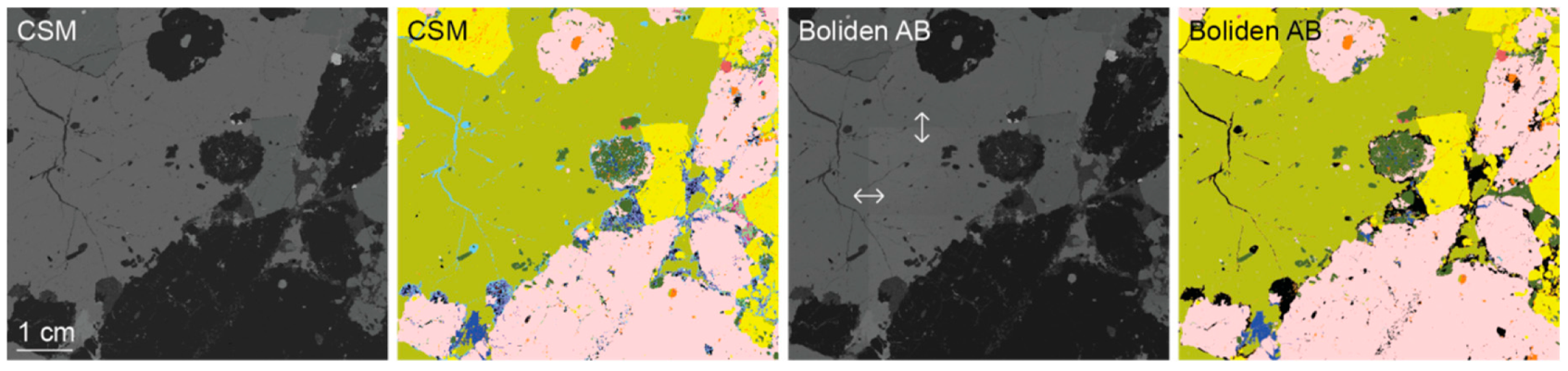
For Boliden AB, the backscattered electron image of the sample area showed several fields with shifts in grey-levels likely caused by poor vacuum conditions or a fluctuating beam current. However, the shifts were not reflected in the mineral map; therefore, the X-ray yield was not significantly affected and/or within the tolerance of the SIP. It is possible that this artefact would have been more problematic in an MLA system, as it relies primarily on the BSE signal for particle distinction. There are a plethora of possible interactions of components within and outside the instrument that can affect vacuum and beam stability, such as vacuum pumps in need of repair and unexpected highs/lows in the power supply or an old filament. Although the results of this analysis were not affected, future complications are possible. Thus, troubleshooting to find the root of the problem is recommended, although it exceeds the scope of this paper.

Regarding the spatial resolution of the scan, CSM opted for a pixel size of 10 µm compared to 5 µm for Boliden AB. The 10 µm resolution was chosen based on the findings of unpublished work by one of the authors (G.K.R.) and a study by Boni et al. [21], which showed the difference between a 10 µm and a 1 µm scan to be marginal from a bulk mineralogical point of view for most samples. Furthermore, this study did not show any significant differences in bulk mineralogy directly attributable to the difference in resolution between Boliden AB and CSM. However, this is deceiving when it comes to the identification and quantification of trace phases. Due to accuracy issues with quantities <100 ppm, no more precise values were reported for many trace phases. In fact, two Au grains detected by Boliden AB (after re-processing the data several times) were misidentified by CSM despite a grain size at CSM scan resolution. Additionally, dependent on the Au signal threshold value in the SIP of Boliden AB, many pixels were erroneously identified as Au. However, all Au grains detected by CSM were confirmed by SEM-EDS. Furthermore, this study showed that with the right SIP, the 5 µm scan at Boliden AB was able to exclude errors and resolve many more Au grains compared to the 10 µm scan at CSM, although quantitatively, they both were below 100 ppm. This means, a scan resolution <10 µm can improve quantification of trace phases if the SIP is of sufficient quality and the data is verified by another method. In fact, for studies focused only on the quantification of Au, even higher resolutions of 1–2 µm are used [8,12,22]. However, this is not realistic with the QEMSCAN^® technology for comprehensive routine analyses of uncrushed samples in the mining industry as the runtime would drastically increase. In this study, the 5 µm scan required already more than twice the amount of time compared to the 10 µm scan. Whether the benefit of a better trace mineral quantification outweighs the downside of a longer scan time is up to the mining company to decide. There is also always the option to follow up a fieldscan with a high-resolution scan in TMS mode or a high-resolution fieldscan of smaller areas of interest.

Concerning mineralogy, the differences between the QEMSCAN^® analyses at Boliden AB and at CSM are apparent. Camborne School of Mines as a research institution has the ambition to achieve the highest level of detail with as little unknowns (“Others”) as possible for every analysis. In this study, 23 phases were distinguished with less than 100 ppm mineral mass that was left unidentified. Most trace minerals were at or below the scan resolution in terms of grain size; however, they were often possible to separate from the surrounding phases and are marked as single pixels in the mineral map. While some single pixels were misclassified, all pixels of valuable trace minerals such as Au and Ag were confirmed by manual SEM-EDS. This was achieved by detailed work with the SIP using the SMART approach [23]. At CSM, the same SIP is used for every sample, regardless of type and origin (geology, archaeology, agriculture, forensics, etc.). However, with every analysis, the SIP is edited and adapted to account for natural compositional variations of minerals between samples. Unknown pixels are individually reviewed to try to deduct the mineral phase (or phases) responsible for the EDS signal and, if successful, a corresponding SIP-entry is added. With detailed mineralogical knowledge of a sample prior to QEMSCAN^® analysis, through thorough optical microscopy and SEM work, the output data will contain much fewer uncertainties. For this study, previous mineralogical studies by Warlo et al. [16] were initially used to better constrain the SIP entries of some phases.

In contrast, for Boliden AB, a rough understanding of the mineralogy of a sample is often considered sufficient. Gangue phases such as silicates, carbonates and oxides have no economic value for the company and similarly, minor and trace ore minerals are often too low in abundance to be economic. Boliden AB, therefore, does not prioritize a detailed characterization and separation of these particular phases. Furthermore, due to the much higher required sample throughput compared to CSM, thorough manual editing of the SIP for every analysis is too time consuming and, therefore, economically unfeasible for Boliden AB. Instead, for each deposit or process-mineralogical type of ore, an individual SIP is developed and consequently, used for the quantitative mineral analysis of the whole deposit. The time it takes to develop a customized SIP is strongly dependent on the mineralogical complexity of the deposit. These customized SIPs are commonly based on prior analysis by optical microscopy. In this case, the SIP for the nearby Aitik Cu-Au deposit was used as a basis due to its somewhat similar mineralogy to the Liikavaara deposit and the SIP being supported by several mineralogical studies even though the two deposits are genetically different. The SIP was then slightly adapted for this particular study, based on previous mineralogical studies by Warlo et al. [16]. The SIP is then typically used for every sample from the same deposit with editing focused mostly on adjusting for mineralogical variations between samples. This saves time (editing of ~14 samples per day) and commonly delivers data of sufficient quality for the mining operation. Nevertheless, the quality of analysis is dependent on how well mineralogy and chemical composition of the minerals in the sample fit with their definitions in the SIP. Major ore minerals are usually well-constrained but especially, mineralogy of gangue and minor and trace phases is not always fully studied/understood and consequently, their SIP-entries are vague or missing.

Furthermore, fine textures with phases smaller than the excitation volume of the electron beam (e.g., trace minerals) commonly produce mixed X-ray signals and thus, are not identified by conventional SIP entries. This explains the shorter mineral list of Boliden AB compared to CSM in this study and the larger variations in modal mineralogy for gangue and trace phases compared to major ore phases. It is also the reason for the amount of unidentified phases. However, although not of economic value, there is definitely a benefit in distinguishing the various gangue phases and trace ore minerals in a sample. The hardness of the gangue phases, for example, dictates crushing of the ore, sheet silicates affect the flotation, and some trace metals are deleterious to primary metals (main commodity). The importance of understanding the mineralogy of trace minerals and gangue minerals especially in Cu-Au ores is also highlighted by Agorhom et al. [24] in their review on trace element recovery in copper flotation. Hence, recognizing these potential problems should be of interest in a mining venture. Boliden AB showed the potential of their QEMSCAN^® system to separate between different gangue phases and minor ore minerals by expanding the mineral list to match CSM. However, it also showcased their limitations caused by a less-developed SIP. Ankerite and jacobsite, for example, could not be differentiated from “Fe-Ox/CO3” since no SIP-entries existed for these phases and no reference material was available to create new entries. To compensate for this less comprehensive SIP compared to CSM and its inability to handle mixed signals and also to deal with signal errors caused by a deflected beam, Boliden AB often applies the “boundary phase processor”. The results showed that it helped to increase similarity in the bulk mineralogy for chalcopyrite between Boliden AB and CSM and to remove falsely classified rims of chalcopyrite around pyrite grains, but at the expense of also removing previously resolved micro-cracks of chalcopyrite. Hence, a comprehensive SIP is a key requirement to high quality and meaningful data. This is, however, not limited to the QEMSCAN^® system. Although the means of mineral identification may differ between ASEM systems, all rely on a comparison of the recorded signal with a database for classification. If minerals are defined by grey-scale values, X-ray intensities, or stoichiometry is marginal. In fact, a study by Kern et al. [25], using the MLA system showed improvements in calculating Sn deportment in a skarn deposit by including mixed phases in their mineral reference list in order to resolve mixed spectra at grain boundaries rather than relying on so-called touchups (similar to a “boundary phase processor”).

Generally, the “scientific” and the “industrial” approach by CSM and Boliden AB, respectively, are both justified for their respective purpose. However, with the rising economic importance of many trace metals and their implications on ore processing and the environment, control over their occurrence and distribution should be of interest to the mining industry and consequently, aimed for with the use of some advanced automated quantitative mineralogical type of analysis. This study explored the potential of routinely identifying economic trace minerals in rocks prior to processing with industrial QEMSCAN^® settings. It was shown that by including single-element SIP-entries as filters at the top of the SIP detection, at best quantification of trace minerals is indeed possible, albeit without being able to distinguish between minerals of similar element composition (e.g., native Au and electrum). One challenge is erroneous signals that cause the misidentification of pixels. While for major ore minerals, Boliden AB utilizes the “boundary phase processor” to correct for these errors, it cannot be applied to trace minerals as they are themselves adversely affected by this method. Instead, a threshold value for the X-ray signal intensity of the trace metal mineral must be added to the single-element SIP-entry. The optimal threshold value to exclude all erroneous signals while including as many true signals as possible may differ between trace metals. To determine the optimal threshold value, QEMSCAN^® data has to be reviewed by other analytical methods, e.g., SEM-EDS to separate true from erroneous pixels. It is not plausible to fully implement this in an industrial routine. However, in this study, even with a threshold value 60% higher than the ideal value (40% compared to 25%), around half of the Au-pixels were captured (20 of 39 pixels). Thus, implementing SIP-entries with conservative threshold values for all economic trace metals in a deposit would already be beneficial with a minimum amount of work. While this, without follow-up analysis, will not provide reliable quantitative mineralogical information and data on grain size and shape, it should provide a basic overview of trace mineral association and distribution and allow for targeted follow-up studies.

5. Conclusions

This study investigated the potential of comprehensive routine quantitative mineralogical characterization of uncrushed rock samples by QEMSCAN^® (as an example of ASEM) in the mining industry, with emphasis on trace mineral quantification. Analytical quality and methodology between an industrial and a scientific application of the QEMSCAN^® system were compared. It was shown that in comparison to a scientific application, the quality of the industry data was largely reliant on the quality of the species identification protocol (SIP) or mineral library used. Especially, the capability to identify different gangue minerals and trace phases and to resolve mixed spectra was inferior for the analysis with settings for an industrial application. The resolution of mixed spectra was achieved through the “boundary phase processor” after modification of the SIP (the preferred method for the scientific analysis) proved too time intensive. It was demonstrated that by modification of the SIP for the analysis using industrial settings, gangue mineral differentiation could be improved. Additionally, the identification and quantification of trace minerals (in this case, Au-minerals) was significantly improved by the addition of single-element entries to the top of the SIP. Due to a potential of erroneous spectra caused by, e.g., a deflected electron beam, a threshold value had to be added to the single-element SIP. The lowest possible threshold value to avoid errors had to be determined experimentally (25% signal intensity for Au) and by verification with another analytical method (SEM-EDS). For a routine application, continuous verification is time consuming and thereby implausible, but a conservative threshold value could be implemented at the expense of missing some pixels of trace minerals. With this method, a 5 µm field scan was able to identify Au grains of less than 2 µm. It was also successfully tested for Ag. However, no information on trace metal mineralogy, grain size, and shape was collected. It thus cannot be compared to the data quality achievable with a 1 µm phase-specific search. However, as an add-on to routine quantitative mineralogical analysis focused on major ore minerals this method can also produce quantitative data and information on mineral association for trace minerals whose metals may be potential by-products in a mining operation. This method will then lay the foundation for further targeted analysis of, for instance, precious- and critical trace metals.

While this study was performed on a single thin section sample only, the method developed to quantify trace minerals should be reproducible for other samples as well. In general, the more complex the mineralogy and textures of a sample and the finer the trace minerals, the more challenging an analysis will be. Additionally, the quality of the analysis is dependent on the quality of polishing (issues with beam deflections). Although this may impact the threshold value necessary to exclude errors, it should not affect the usability of the method itself.

References

1. Study on the Review of the List of Critical Raw Materials; Criticality Assessments; European Commission: Brussels, Belgium, 2017. [CrossRef]
2. Goodall, W.R.; Scales, P.J. An Overview of the Advantages and Disadvantages of the Determination of Gold Mineralogy by Automated Mineralogy. Miner. Eng. 2007, 20, 506–517. [Google Scholar] [CrossRef]
3. Gottlieb, P.; Wilkie, G.; Sutherland, D.; Ho-Tun, E.; Suthers, S.; Perera, K.; Spencer, S.; Butcher, A.; Rayner, J. Using Quantitative Electron Microscopy for Process Mineralogy Applications. Jom 2000, 52, 24–25. [Google Scholar] [CrossRef]
4. Gu, Y. Automated Scanning Electron Microscope Based Mineral Liberation Analysis an Introduction to JKMRC/FEI Mineral Liberation Analyser. J. Miner. Mater. Charact. Eng. 2003, 2, 33–41. [Google Scholar] [CrossRef]
5. Miller, P.; Reid, A.; Zuiderwyk, M. QEM* SEM Image Analysis in the Determination of Modal Assays, Mineral Associations and Mineral Liberation. In Proceedings of the XIV International Mineral Processing Congress, Toronto, ON, Canada, 17–23 October 1982; pp. 1–20. [Google Scholar]
6. Reid, A.; Gottlieb, P.; MacDonald, K.; Miller, P. QEM* SEM Image Analysis of Ore Minerals: Volume Fraction, Liberation, and Observational Variances. In Proceedings of the Second International Congress on Applied Mineralogy in the Minerals Industry, Los Angeles, LA, USA, 22–25 February 1984; Won, C.P., Donald, M.H., Richard, D.H., Eds.; The Metallurgical Society of AIME: Englewood, CO, USA, 1984; pp. 191–204. [Google Scholar]
7. Hall, J. Composite Mineral Particles: Analysis by Automated Scanning Electron Microscopy. Ph.D. Thesis, University of Queensland, Brisbane, Austrilia, 1978. [Google Scholar]
8. Goodall, W.; Scales, P.; Butcher, A.R. The Use of QEMSCAN and Diagnostic Leaching in the Characterisation of Visible Gold in Complex Ores. Miner. Eng. 2005, 18, 877–886. [Google Scholar] [CrossRef]
9. Pirrie, D.; Rollinson, G.K. Unlocking the Applications of Automated Mineral Analysis. Geol. Today 2011, 27, 226–235. [Google Scholar] [CrossRef]
10. Hrstka, T.; Gottlieb, P.; Skála, R.; Breiter, K.; Motl, D. Automated Mineralogy and Petrology-Applications of TESCAN Integrated Mineral Analyzer (TIMA). J. Geosci. 2018, 63, 47–63. [Google Scholar] [CrossRef]
11. Graham, S.D.; Brough, C.; Cropp, A. An Introduction to ZEISS Mineralogic Mining and the Correlation of Light Microscopy with Automated Mineralogy: A Case Study using BMS and PGM Analysis of Samples from a PGE-bearing Chromite Prospect. Precious Met. 2015, 1–12. [Google Scholar]
12. Butcher, A.R.; Helms, T.A.; Gottlieb, P.; Bateman, R.; Ellis, S.; Johnson, N.W. Advances in the Quantification of Gold Deportment by QEMSCAN. In Proceedings of the Seventh Mill Operators Conference, Kalgoorlie, Australia, 12–14 October 2000; pp. 267–271. [Google Scholar]
13. Goodall, W.R. Characterisation of Mineralogy and Gold Deportment for Complex Tailings Deposits Using QEMSCAN®. Miner. Eng. 2008, 21, 518–523. [Google Scholar] [CrossRef]
14. Goodall, W.R.; Butcher, A.R. The Use of QEMSCAN in Practical Gold Deportment Studies. Miner. Process. Extr. Metall. 2012, 121, 199–204. [Google Scholar] [CrossRef]
15. Gy, P. Sampling for Analytical Purposes; John Wiley: New Jersey, NJ, USA, 1998; p. 153. [Google Scholar]
16. Warlo, M.; Wanhainen, C.; Martinsson, O.; Karlsson, P. Mineralogy and Origin of the Intrusion-Related Liikavaara Cu-(W-Au) Deposit, Northern Sweden. GFF 2019. (under review). [Google Scholar]
17. Zweifel, H. Aitik-Geological Documentation of a Disseminated Copper Deposit: A Preliminary Investigation. Ph.D. Thesis, Geological Survey of Sweden, Stockholm, Sweden, 1976. [Google Scholar]
18. Rollinson, G.K.; Andersen, J.C.Ø.; Stickland, R.J.; Boni, M.; Fairhurst, R. Characterisation of Non-Sulphide Zinc Deposits Using QEMSCAN®. Miner. Eng. 2011, 24, 778–787. [Google Scholar] [CrossRef]
19. Warlo, M.; Wanhainen, C.; Bark, G.; Karlsson, P. Gold and Silver Mineralogy of the Liikavaara Cu-(W-Au) Deposit, Northern Sweden. In Proceedings of the 15th SGA Biennial Meeting, Glasgow, UK, 27–30 August 2019. [Google Scholar]
20. Andersen, J.C.Ø.; Rollinson, G.K.; Snook, B.; Herrington, R.; Fairhurst, R. Use of QEMSCAN® for the Characterization of Ni-Rich and Ni-Poor Goethite in Laterite Ores. Miner. Eng. 2009, 22, 1119–1129. [Google Scholar] [CrossRef]
21. Boni, M.; Rollinson, G.; Mondillo, N.; Balassone, G.; Santoro, L. Quantitative Mineralogical Characterization of Karst Bauxite Deposits in the Southern Apennines, Italy. Econ. Geol. 2013, 108(4), 813–833. [Google Scholar] [CrossRef] [Green Version]
22. Agorhom, E.A.; Swierczek, Z.; Skinner, W.; Zanin, M. Combined QXRD-QEMSCAN Mineralogical Analysis of a Porphyry Copper-Gold Ore for the Optimization of the Flotation Strategy. In Proceedings of the XXVI International Mineral Processing Congress (IMPC), New Delhi, India, 23–28 September 2012. [Google Scholar]
23. Haberlah, D.; Owen, M.; Botha, P.W.S.K.; Gottlieb, P. Sem-Eds-Based Protocol for Subsurface Drilling Mineral Identification and Petrological Classification. In Proceedings of the 10th International Congress for Applied Mineralogy (ICAM), Trondheim, Norway, 1–5 August 2011; Springer: Berlin/Heidelberg, Germany, 2012; pp. 265–273. [Google Scholar]
24. Agorhom, E.A.; Lem, J.P.; Skinner, W.; Zanin, M. Challenges and Opportunities in the Recovery/Rejection of Trace Elements in Copper Flotation—A Review. Miner. Eng. 2015, 78, 45–57. [Google Scholar] [CrossRef]
25. Kern, M.; Möckel, R.; Krause, J.; Teichmann, J.; Gutzmer, J. Calculating the Deportment of a Fine-Grained and Compositionally Complex Sn Skarn with a Modified Approach for Automated Mineralogy. Miner. Eng. 2018, 116, 213–225. [Google Scholar] [CrossRef]
Figure 1. (a) Location of the Liikavaara Cu-(W-Au) deposit in Northern Sweden; (b) geological map of the Liikavaara deposit at 100 m below surface. Location of the drill hole for the sample analyzed in this study is shown; (c) thin section prepared from a drill core intersecting a mineralized quartz vein within an aplite dike. Modified from Warlo et al. [16].
Minerals 09 00440 g001
Figure 2. Petrographic images of the thin section analyzed by QEMSCAN® in this study. (a,e) are plane polarized light images, (bd,f) are reflected light images; (a) grains of quartz surrounded by patches of calcite, and pyrrhotite and pyrite; (b) massive pyrrhotite and subhedral pyrite. Sphalerite and chalcopyrite occur along the edges and in cracks of pyrite; (c) scheelite grain within pyrite; (d) grain of pilsenite with patches of pyrrhotite surrounded by calcite; (e) and (f) assemblage of sphalerite, pyrite, calcite and tourmaline surrounded by quartz. Abbreviations: Cal—calcite, Ccp—chalcopyrite, Pil—pilsenite, Po—pyrrhotite, Py—pyrite, Qz—quartz, Sch—scheelite, Sp—sphalerite, Tour—tourmaline.
Minerals 09 00440 g002
Figure 3. Backscattered (ac) and secondary (d) electron images of the thin section prior to QEMSCAN® analysis; (a) intergrowth of native Bi and hessite in a crack between grains of pyrite and sphalerite; (b) droplet-shaped grains of native bismuth with Au in quartz; (c) grains of electrum at the border of sphalerite and tourmaline, respectively; (d) magnified image of (c). Abbreviations: Au—gold, Bi—native bismuth, Cal—calcite, Ccp—chalcopyrite, Chl—chlorite, Ele—electrum, Hes—hessite, Pil—pilsenite, Py—Pyrite, Qz—quartz, Sp—sphalerite, Tour—tourmaline.
Minerals 09 00440 g003
Figure 4. Optical scan of the sample and corresponding QEMSCAN® images (backscattered electrons (BSE) and mineral map) from Camborne School of Mines (CSM) and Boliden AB.
Minerals 09 00440 g004
Figure 5. BSE image and corresponding mineral map of a part of the thin section analyzed in this study for CSM (left) and Boliden AB (right). A grey-level shift in the BSE image of Boliden AB can be observed (indicated by arrows). This shift was not observed for CSM and is not reflected in the mineral map.
Minerals 09 00440 g005
Figure 6. Areas of the QEMSCAN® mineral map by CSM (left) containing pixels identified as electrum (red) and corresponding backscattered electron images of the same areas by FEG-SEM (right). Gold grains detected by CSM and Boliden AB (after reprocessing) are false-colored in the BSE images. The Au grains detected by the CSM scan are also magnified. The magnified images are secondary electron images recorded by FEG-SEM.
Minerals 09 00440 g006
Figure 7. (a–e) Optical microscopy images and corresponding areas in the QEMSCAN® mineral maps of CSM and Boliden AB. In (b), the smaller squares show a magnified image of the underlying area to highlight differences in the micro fracture density between the optical images and the mineral maps. The CSM map includes all the minerals presented in the legend. The original Boliden AB map does not subdivide groups and uses “Silicates” instead of “Biotite”. The final version by Boliden AB uses the same mineral list as CSM but lacks “Ankerite”, “Jacobsite” and subdivision of “Au, Ag minerals”. It includes application of the “boundary phase processor” on chalcopyrite and a single-element entry to the SIP (database) with a 25% intensity threshold for Au.
Minerals 09 00440 g007
Figure 8. Secondary electron images of false-colored gold grains detected by the QEMSCAN® analysis of Boliden AB for a range of signal intensity thresholds (20%–40%) of Au defined in the SIP-entry for the identification of Au minerals. A clear correlation between detectability and size exists. For the grains close to each other, they were marked by a single pixel in the mineral map and it was impossible to discern which had been hit by the electron beam. The grains with an asterisk were also detected by the QEMSCAN® analysis of CSM.
Minerals 09 00440 g008