
Thermoporoelastoplastic Wellbore Breakout Modeling by Finite Element Method

1
School of Mathematics and Physics, University of Science and Technology Beijing, Beijing 100083, China
2
Department of Petroleum Engineering, University of Wyoming, Laramie, WY 82071, USA
3
Geological Survey of Canada, Calgary, AB T2L 2A7, Canada
4
Department of Civil and Environmental Engineering, University of Waterloo, Waterloo, ON N2L 3G1, Canada
*
Author to whom correspondence should be addressed.
Mining 2022, 2(1), 52-64; https://0-doi-org.brum.beds.ac.uk/10.3390/mining2010004
Submission received: 30 September 2021
/
Revised: 6 January 2022
/
Accepted: 20 January 2022
/
Published: 24 January 2022
(This article belongs to the Special Issue Application of Empirical, Analytical, and Numerical Approaches in Mining Geomechanics)
Abstract
:Drilling a hole into rock results in stress concentration and redistribution close to the hole. When induced stresses exceed the rock strength, wellbore breakouts will happen. Research on wellbore breakout is the fundamental of wellbore stability. A wellbore breakout is a sequence of stress concentrations, rock falling, and stress redistributions, which involve initiation, propagation, and stabilization sequences. Therefore, simulating the process of a breakout is very challenging. Thermoporoelastoplastic models for wellbore breakout analysis are rare due to the high complexity of the problem. In this paper, a fully coupled thermoporoelastoplastic finite element model is built to study the mechanism of wellbore breakouts. The process of wellbore breakouts, the influence of temperature and the comparison between thermoporoelastic and thermoporoelastoplastic models are studied in the paper. For the finite element modeling, the D-P criterion is used to determine whether rock starts to yield or not, and the maximum tensile strain criterion is used to determine whether breakouts have happened.
1. Introduction
When a hole is drilled into the crust, the rock mass removed from the hole will not support the surrounding rocks, which leads to the stress concentration and redistribution. If the induced stresses exceed the rock strength, parts of rock fall from the wellbore wall, which is called a wellbore breakout [1,2]. Wellbore breakouts result in problematic wellbore stability and affects drilling efficiency, so the research of wellbore breakouts is important in petroleum engineering [3,4].
Numerous studies have been made to explain the mechanism of wellbore breakouts. Zoback found the analytical solution of initial breakout zone by incorporating the Mohr-Coulomb criterion to the Kirsch equation [2]. The studies of wellbore breakouts show that the wellbore breakouts occur by a series of successive spalls that result from shear failure subparallel to the direction of the local minimum principal stress [3,5,6,7,8,9]. In addition, some studies also show that a wellbore breakout can also influence the wellbore breakdown pressure [10]. To consider the effect of pore pressure and obtain effective stress distribution in a porous medium, Biot [11] proposed a linear poroelastic model based on Terzaghi’s theory and introduced Biot’s coefficient. Later, Fluid seepage and pressure diffusion between the wellbore and the formation were considered for both vertical and inclined wells [12,13,14]. Recently, numerical methods were also used to analyze the breakout mechanisms [15,16,17,18,19].
Most of these models do not consider the influence of plastic damage of the rock. For the plastic model, different yield criteria are used to analyze the character of rock and soil. The Mohr-Coulomb criterion is the most popular one, which relates the shearing resistance to the contact forces and friction [20]. The Drucker-Prager criterion is an extended version of the Von Mises criterion [21]. Whittle and Kavvadas [22] presented the MIT-E3 soil model to describing the behavior of overconsolidated clays that obey normalized behavior and are rate-independent. Akl and Whittle [23] analyzed horizontal wellbore stability in clay shale based on MIT-E3 soil model. Zhang and Yin [24] made a wellbore study using the tangent stiffness matrix method based on the Drucker-Prager criterion.
However, in reality, a wellbore breakout is a complex time-dependent process including initiation, propagation, and stabilization sequences [25]. The breakout initiation and its propagation are the result of stress concentration on the wellbore wall, further stress concentration at the tip of breakout, and the formation of a plastic zone around the tip [26]. Poroelastoplastic analysis of wellbore breakouts is still not well studied due to the complexity of the problem.
With the development of a deep well, consideration of the thermal effects is essential. Coupled thermal-hydraulic-mechanical processes play an important role in the stability of wells in thermal reservoir formations [27]. Lewis [28] used FE simulation to study thermal recovery processes and heat losses problems to surrounding strata. Aboustit et al. [29] used a general variational principle to investigate thermo-elastic consolidation problems, and Vaziri [30] also presented a fully coupled thermo-hydro-mechanical FE model.
In this paper, a fully coupled thermoporoelastoplastic finite element model is built to study the mechanism of wellbore breakouts. The Drucker-Prager criterion is used to determine whether rock starts to yield or not, and the maximum tensile strain criterion is used to determine whether breakouts happened.
2. Model Structure and Methodology
To simulate wellbore breakouts in plastic rock, the Drucker-Prager yield criterion and maximum tensile strain criterion are used to analyze the yield and failure of the rock. The finite element implementation of thermoporoelasticity is based on Biot’s theory with the compressible fluid flowing through the saturated non-isothermal deformable porous medium.
2.1. Rock Failure Criteria
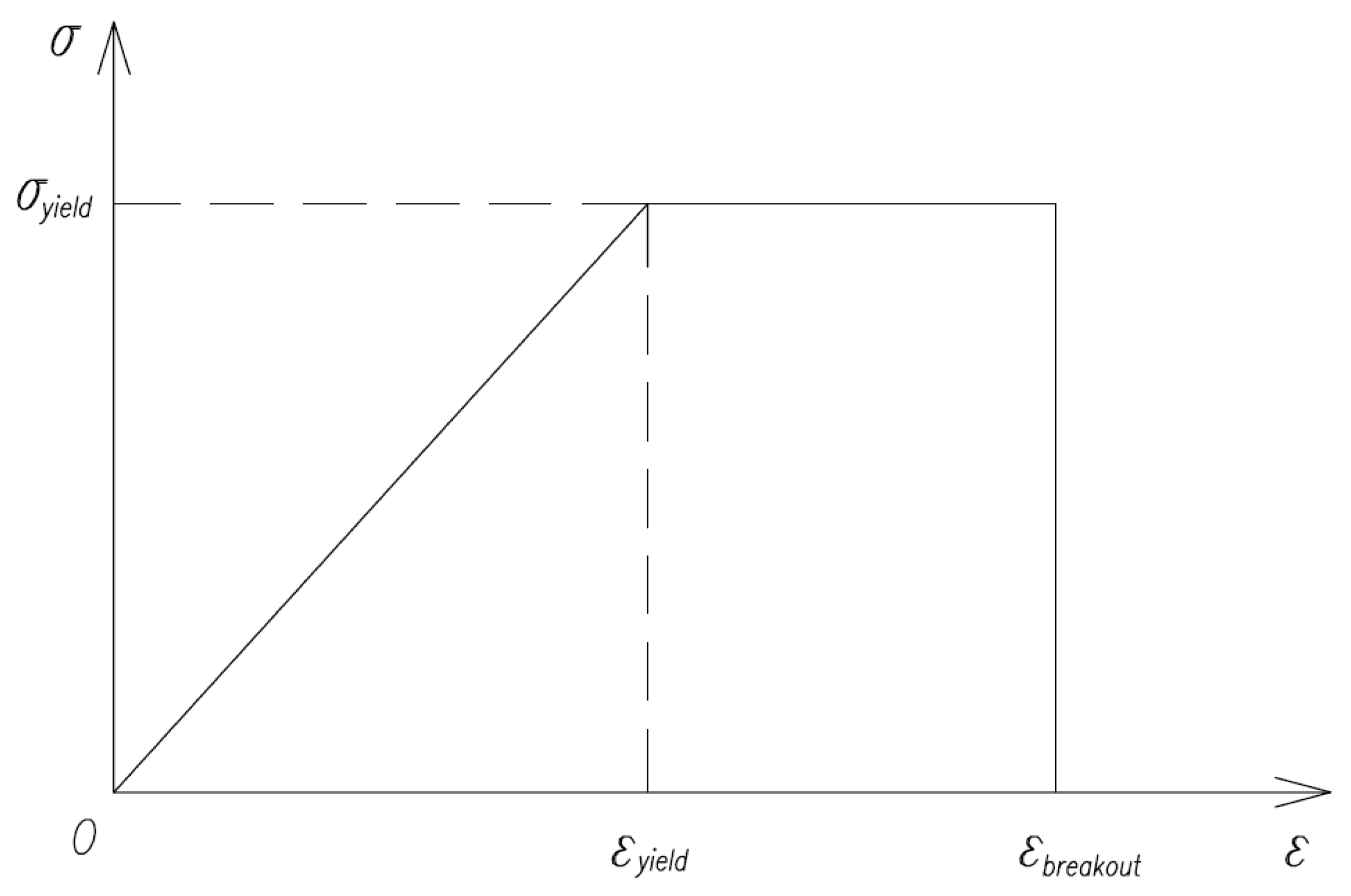
In this paper, the Drucker-Prager yield criterion and maximum tensile strain criterion are used to analyze the yield and failure of the rock. Figure 1 shows a simplified sketch for the relationship between stress and strain in the condition of yield and failure of the rock, where and are the yield stress and strain of rock, is the maximum allowable tensile strain of rock.
The Drucker-Prager yield criterion is an extended version of the Von Mises criterion. To obtain a smooth yield surface approximate to Mohr-Coulomb surface, Drucker and Prager [21] put forward the following yield criterion:
where is is the yield criterion, I1 is the first stress invariant, J2 is the second deviatoric stress invariant, and are the material constants.
Two of the most common approximations used are obtained by making the yield surfaces of the Drucker-Prager and Mohr-Coulomb criteria coincident either at the outer or inner edges of the Mohr-Coulomb surface. Coincidence at the outer edges is obtained when
whereas, coincidence at the inner edges is given by the choice
where is the cohesion of the material; is the internal friction angle of the material.
The yield condition of rock can be determined by the following equation.
The failure (breakout) condition of rock can be determined by the following equation.
2.2. Finite Element Implementation
The general theory of thermoporoelasticity is based on Biot’s theory. With the compressible fluid flowing through the saturated non-isothermal deformable porous medium, in the form of displacements, pressure and temperature as unknowns, the governing equations can be described as follows [31].
where and are the bulk moduli of the skeleton, fluid and matrix, respectively. is the permeability of the porous medium, is the viscosity of the fluid, and are Lamé constants. , and pt denote the displacement of the porous medium, the pore pressure and its time derivative, is the porosity of the porous medium, is the thermal conductivity matrix of the porous media, and Tt are the temperature and time derivative, is the heat capacity of the solid phase, is the heat capacity of the fluid phase, is the thermal expansion coefficient of the matrix, and is the thermal expansion coefficient of the fluid. Furthermore, = [1, 1, 1, 0, 0, 0], and is the elastic stiffness matrix, the subscript denotes time derivative.
Using Galerkin finite element method to approximate the governing equations, the final form of the FEM solution is as follows.
where , are the vectors of unknown variables and corresponding time derivatives, and is the vector for the nodal loads, flow source and heat sources. The explicit expressions of above matrixes are as follows.
To integrate the above equations with respect to time ( method), the equation becomes:
where is the increment of displacement, pore pressure, is the increment vector for the nodal loads and flow source, is the increment of time, is the time integration coefficient, is the initial vector for the nodal loads in a time step, and is the initial vector for the pore pressure in a time step.
If the stresses are in the plastic state at a special time based on the yield criterion, Equation (19) becomes Equation (20) at the special time [32].
where is the set of element nodal forces round the node, and is the unbalanced force. For an ideal elastoplastic body, .
In the process of iteration, the convergence condition can be described as:
where is the norm of vector , and is the convergence precision.
For different iterative methods, the global stiffness matrixes are different, which are shown in Figure 2. For the constant stiffness method, the values in Equation (20) can be calculated based on Equations (10)–(18). For the tangent stiffness method, the explicit expressions of the values in Equation (20) are as follows.
where is elastic-plastic matrix [32,33]. For an ideal elastoplastic body, .
The tangent stiffness method is adopted in this paper.
3. Numerical Experiments
Thermoporoelastoplastic wellbore breakouts are simulated for a vertical well, and there are four parts in this section: the relationship between breakout shape and in situ stresses, verification of wellbore breakout process, influence of drilling fluid temperature, and a comparison between thermoporoelastic and thermoporoelastoplastic modeling.
3.1. Thermoporoelastoplastic Finite Element Modeling of Wellbore Breakouts
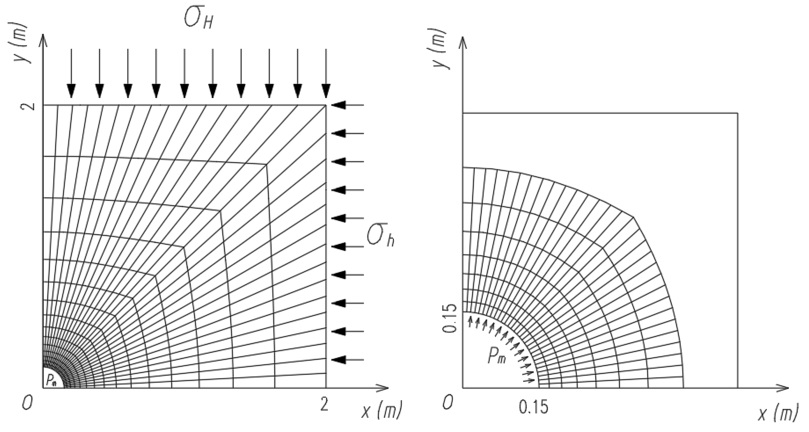
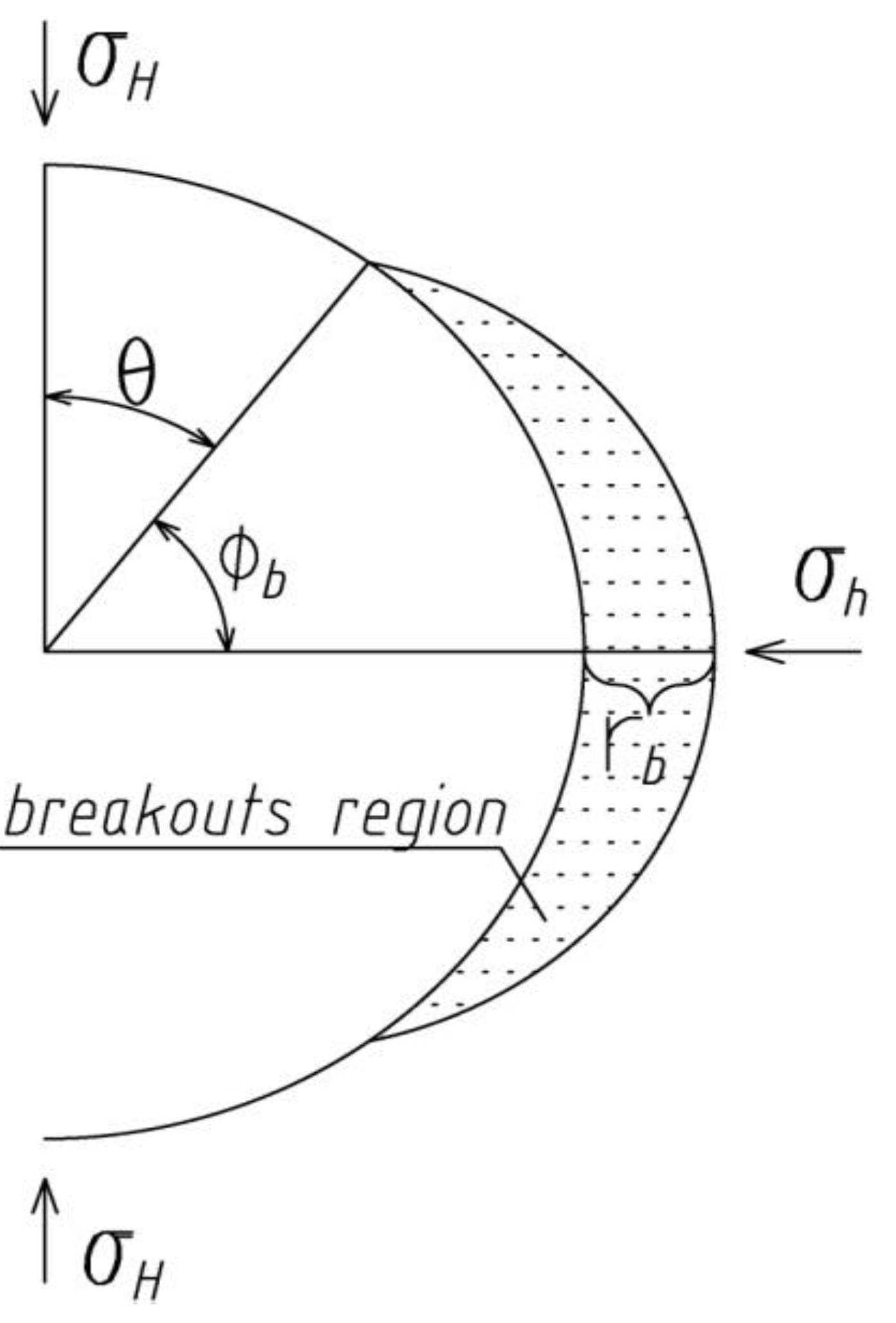
For a vertical wellbore shown in Figure 3 that is subjected to horizontal in-situ stresses and , the shape of breakouts and can be acquired by finite element modeling, where is the depth of breakouts, and is the width of breakouts (Figure 4).
The yield condition of rock is determined by Equation (4), and the failure (breakout) condition of rock is determined by Equation (5).
The geometric and mechanical parameters are shown in Table 1.
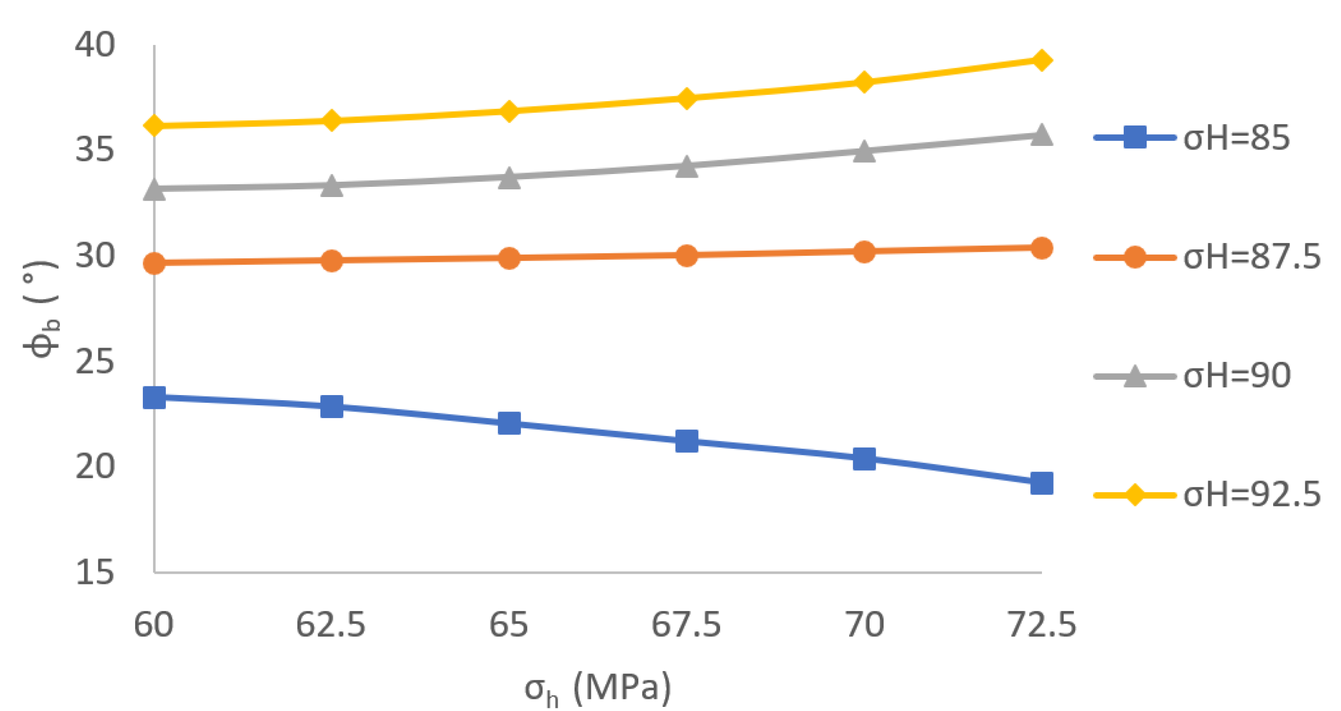
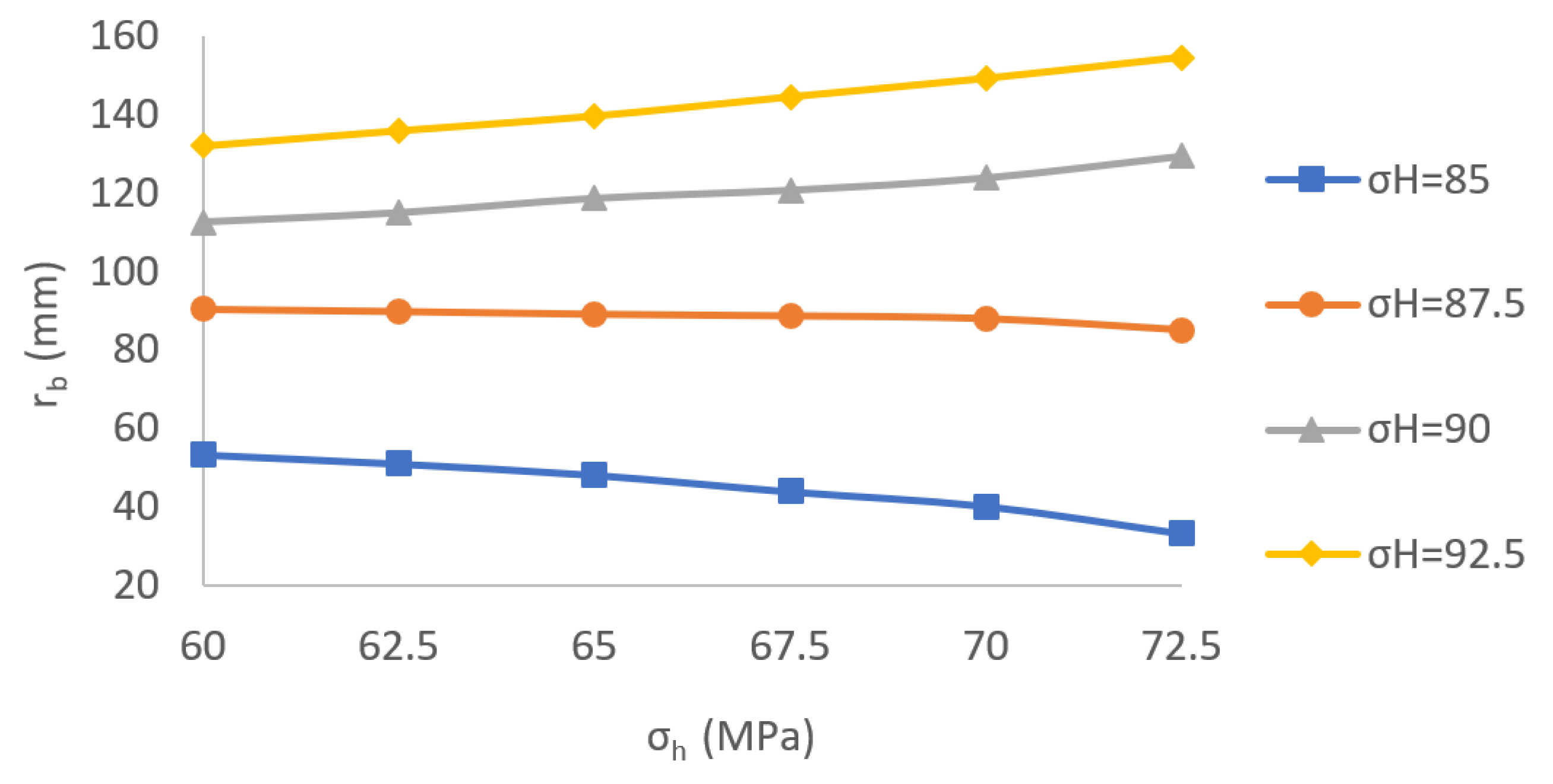
The results of the breakout shape are shown in Table 2. From Table 2, Figure 5 and Figure 6, it can be seen that the relationship between breakout shape and in situ stresses is nonlinear. With relatively large σH and difference between σH and σh, as σh increases, the breakout width and depth increase. With relatively small σH and difference between σH and σh, as σh increases, the difference between σH and σh is smaller, the in situ stress is closer to symmetric in situ stresses state, and the breakout width and depth decrease.
3.2. Verification of Wellbore Breakout Process
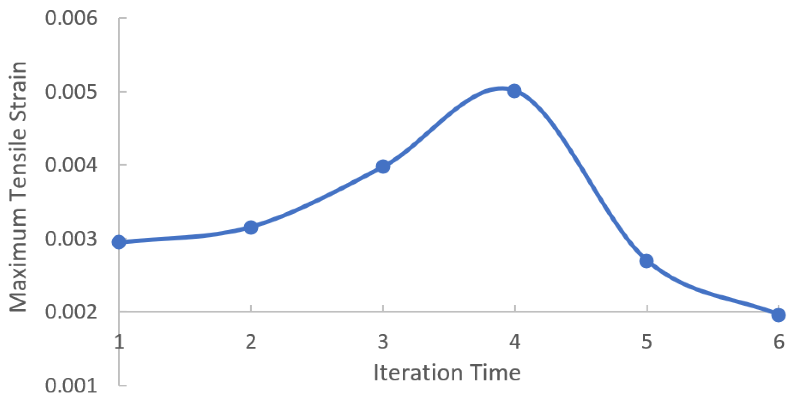
For a vertical well shown in Figure 5, associated with horizontal in situ stresses = 87.5 MPa, = 72.5 MPa and other parameters are listed in Table 1, the process of well breakout is shown in Table 3 and Figure 7, Figure 8 and Figure 9.
From Table 3 and Figure 7, Figure 8 and Figure 9, the principal stresses of elements close to the tip of wellbore breakouts are increasing in the process of breakouts, but the maximum tensile strain changes to less than . As a breakout develops, the breakouts depth increases and the breakout width decreases, which means the depth of breakouts increases till a stable state, but the width of breakouts remains unchanged [3].
3.3. Influence of Drilling Fluid Temperature
For a vertical well shown in Figure 3, associated with horizontal in situ stresses = 85 MPa, = 72.5 MPa, and the temperature difference between drilling fluid and surrounding rock , and other parameters are listed in Table 1, the breakout shape for different drilling fluid temperature is shown in Figure 10.
Based on Figure 10, it can be seen that as temperature of drilling fluid increases, the breakout width and depth will increase.
3.4. Comparison between Thermoporoelastic and Thermoporoelastoplastic Modeling
For a vertical well, shown in Figure 3, which is subjected to horizontal in-situ stresses and , thermoporoelastic and thermoporoelastoplastic modeling are compared in this section, and parameters are listed in Table 1.
For the thermoporoelastoplastic model, the yield condition of rock is determined by Equation (4), and the failure (breakout) condition of rock is determined by Equation (5). For the thermoporoelastic model, the failure (breakout) condition of rock can be determined by Equation (4).
Figure 11 and Figure 12 show different breakout depths and widths corresponding to different in situ stresses by thermoporoelastic and thermoporoelastoplastic modeling.
From Figure 11 and Figure 12, it can be found that for different I -situ stresses, the width and depth of wellbore breakouts for thermoporoelastoplastic model are smaller than those for thermoporoelastic model. For the plastic model, the yield condition of rock is determined by Equation (4), and the failure (breakout) condition of rock is determined by Equation (5). For the elastic model, the failure (breakout) condition of rock can be determined by Equation (4). Therefore, in elastic model, when F > 0 in Equation (4), a breakout happens, but in plastic model, rocks just enter plastic state and no breakouts happened. Therefore, the breakout widths and depths are greater for the elastic model compared to the plastic model.
4. Discussion
In this paper, wellbore breakout process is simulated by the finite element method. Plasticity and temperature influence are considered, and results are compared with elastic model. There are some limits for this study. First, mud cake is assumed to be perfect, and there is no liquid transfer across the mud cake. Second, ideal elastictoplastic stress-strain relationship is used. Third, results are not verified by experimental data and field data. Future work is expected to address this in the next step.
5. Conclusions
In this paper, the finite element method is employed to simulate wellbore breakouts based on the thermoporoelastoplastic model. Numerical experiments on finite element modeling of wellbore breakouts show the contrasting tendency of breakouts shape with different in situ stress, and some conclusions can be made as follows:
- The relationship between breakout shape and in situ stresses is nonlinear. If the is constant, as increases, the breakout width and depth become greater. If the is kept constant while the difference between and is relatively large, as increases, the breakout width and depth increase greater. However, if the is kept constant while the difference between and is relatively small, as increases, the breakout width and depth decrease instead.
- In the process of wellbore breakouts, the breakout depth increases till a stable state, but the breakout width remains unchanged.
- As temperature of drilling fluid increases, the breakout width and depth will increase.
- For different in situ stresses, the width and depth of wellbore breakouts for thermoporoelastoplastic model are smaller than those for thermoporoelastic model.
Author Contributions
L.Z. and H.Z.: modeling; K.H., Z.C. and S.Y.: supervision. All authors have read and agreed to the published version of the manuscript.
Funding
This research received no external funding.
Data Availability Statement
Not applicable.
Conflicts of Interest
The authors declare no conflict of interest.
References
- Bell, J.S. The stress regime of the scotian shelf offshore eastern Canada to 6 km depth and implications for rock mechanics and hydrocarbon migration. Int. J. Rock Mech. Min. Sci. Geomech. Abstr. 1991, 28, A88. [Google Scholar]
- Zoback, M.D.; Moos, D.L.; Mastin, L.; Anderson, R.N. Wellbore breakout and insitu stress. J. Geophys. Res. 1985, 90, 5523–5538. [Google Scholar] [CrossRef]
- Zheng, Z.; Kemeny, J.; Cook, N.G.W. Analysis of borehole breakouts. J. Geophys. Res. 1989, 94, 7171–7182. [Google Scholar] [CrossRef]
- Ito, T.; Zoback, M.D.; Peska, P. Utilization of mud weights in excess of the least principal stress to stabilize wellbores: Theory and practical examples. SPE Drill. Complet. 2001, 16, 221–229. [Google Scholar] [CrossRef]
- Haimson, B.C.; Herrick, C.G. In situ stress evaluation from borehole breakouts experimental studies. In Proceedings of the 26th US Rock Mechanics Symposium, Rapid City, South Dakota, 10 June 1985; Balkema: Rotterdam, The Netherlands, 1985; pp. 1207–1218. [Google Scholar]
- Haimson, B.C.; Herrick, C.G. Borehole breakouts-a new tool for estimating in situ stress? In Proceedings of the First International Symposium on Rock Stress and Rock Stress Measurement, Stockholm, Sweden, 1–3 September 1986; Centek Publications: Lulea, Sweden, 1986; pp. 271–281. [Google Scholar]
- Haimson, B.C. Micromechanisms of borehole instability leading to breakouts in rocks. Int. J. Rock Mech. Min. Sci. 2007, 44, 157–173. [Google Scholar] [CrossRef]
- Papamichos, E. Borehole failure analysis in a sandstone under anisotropic stresses. Int. J. Numer. Anal. Methods Geomech. 2010, 34, 581–603. [Google Scholar] [CrossRef]
- Yuan, S.C.; Harrison, J.P. Modeling breakout and near-well fluid flow of a borehole in an anisotropic stress field. In Proceedings of the 41st ARMA/USRMS, Golden, Colorado, 17–21 June 2006; pp. 6–1157. [Google Scholar]
- Zhang, H.; Yin, S.; Aadnoy, B.S. Numerical investigation of the impacts of borehole breakouts on breakdown pressure. Energies 2019, 12, 888. [Google Scholar] [CrossRef] [Green Version]
- Biot, A. General theory of three dimensional consolidations. J. Appl. Phys. 1941, 12, 155–164. [Google Scholar] [CrossRef]
- Bratli, R.K.; Horsrud, P.; Risnes, R. Rock mechanics applied to the region near a wellbore. In Proceedings of the 5th ISRM Congress, International Society for Rock Mechanics, Melbourne, Australia, 10 April 1983. [Google Scholar]
- Abousleiman, Y.; Roegiers, J.C.; Cui, L.; Cheng, A.H.D. Poroelastic solution of an inclined borehole in a transversely isotropic medium. In Proceedings of the 35th U.S. Symposium on Rock Mechanics (USRMS), American Rock Mechanics Association, Lake Tahoe, CA, USA, 1 January 1995. [Google Scholar]
- Cui, L.; Cheng, A.H.D.; Abousleiman, Y. Poroelastic solution for an inclined borehole. J. Appl. Mech. 1997, 64, 32–38. [Google Scholar] [CrossRef]
- Fakhimi, A.; Carvalho, F.; Ishida, T.; Labuz, J.F. Simulation of failure around a circular opening in rock. Int. J. Rock Mech. Min. Sci. 2002, 39, 507–515. [Google Scholar] [CrossRef]
- Cook, B.K.; Lee, M.Y.; DiGiovanni, A.A.; Bronowski, D.R.; Perkins, E.D.; Williams, J.R. Discrete element modeling applied to laboratory simulation of near-wellbore mechanics. Int. J. Geomech. 2004, 4, 19–27. [Google Scholar] [CrossRef]
- Rahmati, H. Micromechanical Study of Borehole Breakout Mechanism. Ph.D. Thesis, University of Alberta, Edmonton, AB, Canada, 2013. [Google Scholar]
- Mostafa, G.; Goodarznia, I.; Shadizadeh, S.R. Transient thermo-poroelastic finite element analysis of borehole breakouts. Int. J. Rock Mech. Min. Sci. 2014, 71, 418–428. [Google Scholar]
- Lee, H.; Moon, T.; Haimson, B.C. Borehole breakouts induced in Arkosic sandstones and a discrete element analysis. Rock Mech. Rock Eng. 2016, 49, 1369–1388. [Google Scholar] [CrossRef]
- Jaeger, J.C.; Cook, N.G.W. Fundamentals of Rock Mechanics; Chapman & Hall: London, UK, 1979. [Google Scholar]
- Drucker, D.C.; Prager, W. Soil mechanics and plastic analysis for limit design. Q. Appl. Math. 1952, 10, 157–165. [Google Scholar] [CrossRef] [Green Version]
- Whittle, A.J.; Kavvadas, M. Formulation of the MIT-E3 constitutive model for overconsolidated clays. J. Geotech. Eng. 1994, 120, 173–198. [Google Scholar] [CrossRef]
- Akl, S.A.; Whittle, A.J. Analysis of horizontal wellbore stability in clay shale. In Proceedings of the 46th US Rock Mechanics/Geomechanics Symposium, Chicago, IL, USA, 24–27 June 2012. ARMA12-559. [Google Scholar]
- Zhang, H.; Yin, S. Poroelastoplastic borehole modeling by tangent stiffness matrix method. Int. J. Geomech. 2020, 20, 04020010. [Google Scholar] [CrossRef]
- Li, X.; ELMohtar, C.S.; Gray, K.E. Numerical modeling of borehole breakout in ductile formation considering fluid seepage and damage-induced permeability change. In Proceedings of the 50th US Rock Mechanics/Geomechanics Symposium, Houston, TX, USA, 26–29 June 2016. ARMA16-244. [Google Scholar]
- Mastin, L. The Development of Borehole Breakouts in Sandstone. Master’s. Thesis, Stanford University, Stanford, CA, USA, 1984. [Google Scholar]
- Yin, S.; Towler, B.F.; Dusseault, M.B.; Rothenburg, L. Fully coupled THMC modeling of wellbore stability with thermal and solute convection considered. Transp. Porous Media 2010, 84, 773–798. [Google Scholar] [CrossRef]
- Lewis, R.W.; Majorana, C.E.; Schrefler, B.A. A coupled finite element model for the consolidation of non-isothermal elastoplastic porous media. Transp. Porous Media 1986, 1, 155–178. [Google Scholar] [CrossRef]
- Aboustit, B.L.; Advani, S.H.; Lee, J.K. Variational principles and finite element simulations for thermo-elastic consolidation. Int. J. Numer. Anal. Methods Geomech. 1985, 9, 49–69. [Google Scholar] [CrossRef]
- Vaziri, H.H.; Britto, A.M. Theory and application of a fully coupled thermalhydro-mechanical finite-element model. Comput. Struct. 1996, 61, 131–146. [Google Scholar]
- Yin, S. Geomechanics-Reservoir Modeling by Displacement Discontinuity-Finite Element Method. Ph.D. Thesis, University of Waterloo, Waterloo, ON, Canada, 2008; pp. 22–23. [Google Scholar]
- Zhu, B. The Finite Element Method; Tsinghua University Press: Beijing, China, 2018. [Google Scholar]
- Neto, E.S.; Peric, D.; Owen, D. Computational Methods for Plasticity; Wiley: Chichester, UK, 2008. [Google Scholar]
Figure 1.
Sketch of the stress-strain relationship.

Figure 2.
(A) Constant stiffness method, (B) Tangent stiffness method.

Figure 3.
Mesh of finite element model.

Figure 4.
Schematic of a wellbore breakout shape.

Figure 5.
Breakout width for different in situ stresses.

Figure 6.
Breakout depth for different in situ stresses.

Figure 7.
Principal stresses for the element in the breakout tip in the process of breakouts.

Figure 8.
Maximum strain in the breakout tip in the process of breakouts.

Figure 9.
Changing of breakout region in the process of breakouts.

Figure 10.
Breakout width and depth for different drilling fluid temperature.

Figure 11.
Comparison of breakout width between thermoporoelastic and thermoporoelastoplastic model.
Figure 11.
Comparison of breakout width between thermoporoelastic and thermoporoelastoplastic model.

Figure 12.
Comparison of breakout depth between thermoporoelastic and thermoporoelastoplastic model.
Figure 12.
Comparison of breakout depth between thermoporoelastic and thermoporoelastoplastic model.


Table 1.
Geometric and mechanical parameters.
| Parameter | Value |
|---|---|
| Young’s Modulus, (MPa) | 14,400 |
| Poisson Ratio, | 0.2 |
| Cohesion, (MPa) | 6 |
| Inner friction angle, (°) | 35 |
| Radius of well, | 0.15 |
| Bulk modulus of skeleton, | 8000 |
| Bulk modulus of matrix, | 36,000 |
| Bulk modulus of fluid, | 2250 |
| Porosity of the porous medium, | 0.19 |
| Permeability of the porous medium, | 0.19 |
| Viscosity of the fluid, | 10−9 |
| Thermal conductivity, | 2.5 |
| Thermal expansion coefficient of solid, | 2.1 × 10⁻⁵ |
| Thermal expansion coefficient of liquid, | 2.0 × 10⁻⁴ |
| Specific heat of solid, | 800 |
| Specific heat of liquid, | 4200 |
| Maximum principal stress, | 85~92.5 |
| Minimum principal stress, | 60~72.5 |
| Vertical stress, | 80 |
| Drilling fluid pressure, | 45 |
| Temperature difference between drilling fluid and surrounding, | −50 |
| Maximum allowable tensile strain, | 0.002 |
Table 2.
Result of the shape of wellbore breakouts and by FEM.
| No. | σh | σH | rb | No. | σh | σH | rb | ||
|---|---|---|---|---|---|---|---|---|---|
| MPa | MPa | ° | mm | MPa | MPa | ° | mm | ||
| 1 | 85.0 | 60.0 | 23.3 | 53.5 | 13 | 90.0 | 67.5 | 33.2 | 112.7 |
| 2 | 85.0 | 62.5 | 22.9 | 51.2 | 14 | 90.0 | 70.0 | 33.3 | 115.1 |
| 3 | 85.0 | 65.0 | 22.1 | 48.3 | 15 | 90.0 | 72.5 | 33.7 | 118.8 |
| 4 | 85.0 | 67.5 | 21.2 | 44.1 | 16 | 90.0 | 60.0 | 34.3 | 120.9 |
| 5 | 85.0 | 70.0 | 20.4 | 40.3 | 17 | 90.0 | 62.5 | 35.0 | 124.0 |
| 6 | 85.0 | 72.5 | 19.3 | 33.4 | 18 | 90.0 | 65.0 | 35.8 | 129.6 |
| 7 | 87.5 | 60.0 | 29.7 | 90.6 | 19 | 92.5 | 67.5 | 36.2 | 132.2 |
| 8 | 87.5 | 62.5 | 29.8 | 90.1 | 20 | 92.5 | 70.0 | 36.4 | 136.1 |
| 9 | 87.5 | 65.0 | 29.9 | 89.3 | 21 | 92.5 | 72.5 | 36.9 | 139.8 |
| 10 | 87.5 | 67.5 | 30.0 | 88.9 | 22 | 92.5 | 60.0 | 37.5 | 144.6 |
| 11 | 87.5 | 70.0 | 30.2 | 88.2 | 23 | 92.5 | 62.5 | 38.2 | 149.3 |
| 12 | 87.5 | 72.5 | 30.4 | 85.2 | 24 | 92.5 | 65.0 | 39.3 | 154.6 |
Table 3.
Data of effective principal stresses and breakout region in the process of breakouts.
| Elem | Iteration1 | Iteration2 | Iteration3 | |||||||||
| σ1′ (MPa) | σ2′ (MPa) | σ3′ (MPa) | εmax | σ1′ (MPa) | σ2′ (MPa) | σ3′ (MPa) | εmax | σ1′ (MPa) | σ2′ (MPa) | σ3′ (MPa) | εmax | |
| 1 | −19.64 | −87.86 | −54.31 | 0.00294 | −20.56 | −91.03 | −55.97 | 0.00315 | −28.26 | −113.46 | −66.27 | 0.00397 |
| 2 | −19.86 | −87.44 | −54.21 | 0.00292 | −20.79 | −90.46 | −55.86 | 0.00314 | −28.98 | −111.17 | −65.55 | 0.00387 |
| 3 | −20.29 | −86.59 | −54.00 | 0.00288 | −21.28 | −89.41 | −55.64 | 0.00311 | −30.35 | −106.72 | −64.05 | 0.00362 |
| 4 | −20.93 | −85.35 | −53.70 | 0.00282 | −21.97 | −87.94 | −55.30 | 0.00305 | −31.98 | −99.88 | −61.76 | 0.00328 |
| 5 | −21.73 | −83.74 | −53.31 | 0.00275 | −23.08 | −86.13 | −54.89 | 0.00295 | −33.25 | −90.66 | −58.60 | 0.00290 |
| 6 | −22.67 | −81.78 | −52.84 | 0.00266 | −24.60 | −84.05 | −54.28 | 0.00277 | −33.25 | −79.86 | −54.76 | 0.00236 |
| 7 | −23.71 | −79.54 | −52.31 | 0.00257 | −26.56 | −81.64 | −53.33 | 0.00248 | −29.37 | −64.73 | −48.08 | 0.00168 |
| 8 | −24.85 | −77.08 | −51.74 | 0.00246 | −27.60 | −78.51 | −51.49 | 0.00211 | −25.69 | −53.71 | −43.49 | 0.00133 |
| 9 | −26.13 | −74.51 | −51.08 | 0.00231 | −27.75 | −73.95 | −50.08 | 0.00191 | −23.57 | −49.53 | −40.89 | 0.00094 |
| 10 | −27.67 | −71.91 | −50.22 | 0.00205 | −27.14 | −66.88 | −48.84 | 0.00199 | −23.10 | −47.39 | −40.83 | 0.00091 |
| Elem | Iteration4 | Iteration5 | Iteration6 | |||||||||
| σ1′ (MPa) | σ2′ (MPa) | σ3′ (MPa) | εmax | σ1′ (MPa) | σ2′ (MPa) | σ3′ (MPa) | εmax | σ1′ (MPa) | σ2′ (MPa) | σ3′ (MPa) | εmax | |
| 1 | −44.48 | −142.16 | −85.00 | 0.00501 | −73.96 | −174.26 | −101.91 | 0.00270 | −89.52 | −181.38 | −111.19 | 0.00196 |
| 2 | −44.71 | −128.38 | −76.66 | 0.00523 | −64.49 | −137.95 | −83.14 | 0.00305 | −58.62 | −116.89 | −72.32 | 0.00194 |
| 3 | −42.72 | −108.77 | −70.07 | 0.00433 | −39.34 | −69.62 | −54.19 | 0.00185 | −25.22 | −50.52 | −42.48 | 0.00083 |
| 4 | −40.12 | −87.33 | −61.17 | 0.00323 | −17.79 | −38.71 | −37.73 | 0.00080 | −15.15 | −29.09 | −35.71 | −0.00004 |
| 5 | −32.66 | −62.74 | −49.07 | 0.00195 | −17.15 | −29.80 | −36.13 | −0.00007 | −15.68 | −26.52 | −35.48 | −0.00014 |
| 6 | −23.86 | −45.66 | −40.42 | 0.00097 | −16.17 | −27.53 | −35.79 | −0.00006 | −15.10 | −24.65 | −34.91 | −0.00012 |
| 7 | −20.75 | −38.00 | −37.25 | 0.00014 | −15.95 | −25.85 | −35.30 | −0.00008 | −15.20 | −23.19 | −34.55 | −0.00014 |
| 8 | −19.36 | −36.17 | −37.26 | 0.00020 | −16.14 | −25.73 | −35.25 | −0.00006 | −15.57 | −23.52 | −34.70 | −0.00013 |
| 9 | −19.50 | −36.24 | −37.52 | 0.00019 | −16.71 | −26.65 | −35.51 | −0.00006 | −16.02 | −24.40 | −34.95 | −0.00012 |
| 10 | −19.25 | −36.35 | −37.60 | 0.00020 | −16.87 | −27.24 | −35.63 | −0.00004 | −16.25 | −25.08 | −35.11 | −0.00010 |
Publisher’s Note: MDPI stays neutral with regard to jurisdictional claims in published maps and institutional affiliations. |
© 2022 by the authors. Licensee MDPI, Basel, Switzerland. This article is an open access article distributed under the terms and conditions of the Creative Commons Attribution (CC BY) license (https://creativecommons.org/licenses/by/4.0/).
Share and Cite
MDPI and ACS Style
Zhang, L.; Zhang, H.; Hu, K.; Chen, Z.; Yin, S. Thermoporoelastoplastic Wellbore Breakout Modeling by Finite Element Method. Mining 2022, 2, 52-64. https://0-doi-org.brum.beds.ac.uk/10.3390/mining2010004
AMA Style
Zhang L, Zhang H, Hu K, Chen Z, Yin S. Thermoporoelastoplastic Wellbore Breakout Modeling by Finite Element Method. Mining. 2022; 2(1):52-64. https://0-doi-org.brum.beds.ac.uk/10.3390/mining2010004
Chicago/Turabian StyleZhang, Lijing, Hua Zhang, Kezhen Hu, Zhuoheng Chen, and Shunde Yin. 2022. "Thermoporoelastoplastic Wellbore Breakout Modeling by Finite Element Method" Mining 2, no. 1: 52-64. https://0-doi-org.brum.beds.ac.uk/10.3390/mining2010004