Modelling and Planning Evolution Styles in Software Architecture †


1
LS2N-UMR CNRS 6004, 44300 Nantes, France
2
FST-USTTB, University of Science, Techniques and Technology, Bamako, BPE 3206, Mali
*
Author to whom correspondence should be addressed.
†
This paper is the extension of the conference paper: Djibo, K.; Oussalah, M. and Konate, J. Evolution Style Mining in Software Architecture. In Proceedings of the 15th International Conference on Evaluation of Novel Approaches to Software Engineering, Prague, Czech Republic, 5–6 May 2020.
Modelling 2020, 1(1), 53-76; https://0-doi-org.brum.beds.ac.uk/10.3390/modelling1010004
Submission received: 21 July 2020
/
Revised: 31 August 2020
/
Accepted: 11 September 2020
/
Published: 15 September 2020
(This article belongs to the Special Issue Feature Papers of Modelling)
Abstract
:The purpose of this study is to find the right model to plan and predict future evolution paths of an evolving software architecture based on past evolution data. Thus, in this paper, a model to represent the software architecture evolution process is defined. In order to collect evolution data, a simple formalism allowing to easily express software architecture evolution data is introduced. The sequential pattern extraction technique is applied to the collected evolution styles of an evolving software architecture in order to predict and plan the future evolution paths. A learning and prediction model is defined to generate the software architecture possible future evolution paths. A method for evaluating the generated paths is presented. In addition, we explain and validate our approach through a study on two examples of evolution of component-oriented software architecture.
1. Introduction
Software systems are becoming more complex day after day, and integrate many components. Thus, some research has focused on planning and prediction of software evolution [1,2,3,4]. However, software architectures go hand in hand with the software products they document, they evolve together and constantly. While a lot of works have been directed towards the problem of reusing the evolution of software architectures [5,6,7,8], it is very tedious to evolve the architecture of complex systems (distributed systems, some embedded systems, etc.). The best would be to plan and predict the future evolution paths of an evolving software architecture based on data from previous changes. So, little work has focused on the problem of planning and prediction of the future evolution of software architectures. The majority of research efforts focused on the specification, development, deployment of software architectures [9,10,11] and the analysis, design and reuse of the software architectures evolution [6,12]. However, little works, to our knowledge, are devoted to planning and prediction of futures evolutions paths in software architectures.
From previous evolution data of an evolving architecture over time to , the problem is to determine the recurrent evolution sequences, the architectural elements most or least affected in order to identify and propose the possibilities and skills required to move towards . To achieve this goal, we reuse the evolution style approach introduced by Oussalah et al., 2006 in order to make the process of software architecture evolution reusable and the sequentials patterns extraction techniques to determine recurrent evolution styles. In this paper, our goal is to define a generic approach to predict and plan the future evolution paths of a component-oriented software architecture. Thus, following previous evolutions of software architectures, we build libraries of evolution styles from which we extract the sequential patterns of software architectures evolution. To do this, we define a simple formalism to express the evolution styles with more convenience. Sequentials patterns extraction technique as introduced in [13] is applied to an evolving software architecture evolution styles expressed according to the defined formalism, to extract the software architecture evolution sequentials patterns in order to predict and plan the software architecture future evolution paths. The sequential patterns extraction is a very important area of data mining. It has been used in several studies on specific types of data including the web [14], music [15], software engineering [16,17,18,19], ontology [20], medicine [21]. However, the main challenge in extracting sequential patterns is related to the high costs of processing due to the large amount of data. Thus different algorithms have been proposed in previous studies to optimize data processing costs to determine sequential patterns [13,22,23,24,25,26]. In this paper, we use the principles of sequential patterns extraction on software architectures evolution styles expressed through the formalism that we defined in order to determine the software architecture evolution sequentials patterns. By analogy with the approach of Agrawal et al. in [13], we reorganize the data (the evolution styles expressed) into a seven-field table where we associate with an architectural element, the date of evolution operation undergone, the name, the evolution style header. From this table, we define an algorithm to define evolution sequences by architectural element, then we determine the sequential patterns that define the recurrent evolution sequences. We define another algorithm that, based on a database of evolution sequences, determines the evolution rate of architectural elements and the participation rate of actors in evolution operations. We explain our approach through a study on two examples of component-oriented software architecture evolution. In this study, we are interested in the evolution of the structure of architecture.
This paper is organized as follows: Bellow related work on software architecture evolution, software architecture evolution planning and prediction solutions and knowledge extraction from data (data mining) is presented. In Section 2, we present the case study on which the approach will be applied. The Section 3 presents the introduced evolution model. The planning model is presented in Section 4. The proposed prediction methodology is explained in the Section 5. Finally in Section 6, we conclude and give the perspectives of our work.
1.1. Related Work
Some existing work related to software architecture evolution styles and data mining are presented below.
1.1.1. Architecture Evolution
Much work has been proposed to support the architect in the process of software architecture evolution. In this document, we will limit ourselves to present the work by team on the evolution style approach.
An evolution style captures a characteristic way of evolving all or part of a software architecture. It serves as a guide for an architect who must conform to the style [27]. Evolution styles aim to make the evolution activity reusable to prevent architects from starting from scratch with each evolution activity. They promote knowledge sharing but also learning and knowledge extraction. We present some team approaches. According to [28], an evolution style expresses the evolution of software architecture as a set of potential evolution paths from the initial architecture to the target architecture. Each path defines a sequence of evolution transitions, each of which is specified by evolution operators. In [12], the authors defined evolution styles based on architectural knowledge (AKdES), which are also based on architecture design decisions each time an evolution step is made. Each stage of evolution is preformed because a decision of evolution is taken following the verification of an evolution decision. According to [27], the main idea of an evolution style is to model software architecture evolution activity in order to provide reusable expertise of domain-specific evolution. They consider an architectural evolution as consisting of modifications (addition, update, deletion) of architectural elements (component, connector, interface).
1.1.2. Software Architecture Evolution Planning and Prediction Solutions
In [29], the authors proposed a method and the accompanying tool set to aid the user in selecting the “best” evolution alternative. The user specifies the desired types of evolutions and inputs the initial architecture (also specified in xADL). The proposed tools, first, convert the initial architecture to a graph and, then, fetch architectural changes (from the repository) whose categories match the desired evolutions. Next, the evolution alternatives are generated with a graph transformation tool. Quality attributes are evaluated for each evolution alternative based on the impact of different architectural changes. Finally, the user can query and score the evolution alternatives according to the desired structural and path properties.
In [30], Garlan et al. presented an approach for automated generation of software architecture evolution path. Their approach is much more goal-directed. Instead of beginning with the initial architecture and blindly applying operators in the hope of attaining a suitable path with a suitable end state, they begin by defining both the initial architecture and the target architecture. Then, they use a planner to generate a path by which the initial architecture can be evolved into the target architecture.
1.1.3. Extracting Knowledge from Data (Data Mining)
Extracting knowledge from data (data mining) has been used in many areas to find patterns to solve decision-making or future projection problems in companies. We then present some work done in this direction. Agrawal et al. [13], introduced the sequential pattern discovery problem. From a database of client transactions, they define a sequence database where each sequence represents all the items purchased during a transaction. It was a question of discovering all the sequential patterns with a specified minimum support. They defined three algorithms to solve the problem including the AprioriAll, AprioriSome and DynamicSome algorithms. In 1996, the same team proposed an improvement of the previous result with three modifications as follows: First, they add time constraints that specify a minimum and/or maximum time period between adjacent elements of a pattern. Second They relax the restriction that the items of an element of a sequential pattern must come from the same transaction, allow the elements to be present in a set of transactions whose transaction time is within a time window defined by the user. Third, given that a user-defined taxonomy (is a hierarchy) on items, they allow sequential patterns to include items at all levels of taxonomy [22]. The authors present the GSP algorithm for the discovery of generalized sequential patterns. A performance evaluation performed in [22] indicates that GSP is performing better than AprioriAll presented in [13]. In [20] the change of ontology was studied. They analyze ontology change logs represented as graphs to determine frequent and recurring changes. These frequent and recurring changes are identified as patterns of change that can be reused. For this, they introduced two algorithms to determine ontology change patterns, which are the algorithm for searching complete and ordered change patterns (OCP) and the search algorithm for complete and unordered change patterns ( PCU). They then performed a performance study of the two algorithms to determine the different limitations.
The new approach that we introduce to express and analyze software architectures evolution styles in order to predict and plan future evolutions of theses is presented below. In order to better explain our approach, we open a case study in the following section.
2. Case Study
In this section, the proposed methodology and the three models defined to respectively represent software architecture evolution process, analyze evolution data and predict future evolution path are applied on two examples of trivial and non-trivial component-oriented software architecture evolution that we present.
2.1. Goal
The objective of this study is to find the right models to respectively represent and plan the software architecture evolution process and the right methodology to predict future evolution paths of an evolving Component-Oriented software architecture based on past evolution data.
Starting from an initial architecture evolving to , it is a question of using the data of evolutions from to to propose to the architect the possibilities and to define a principle of evaluation of each proposed possibility.
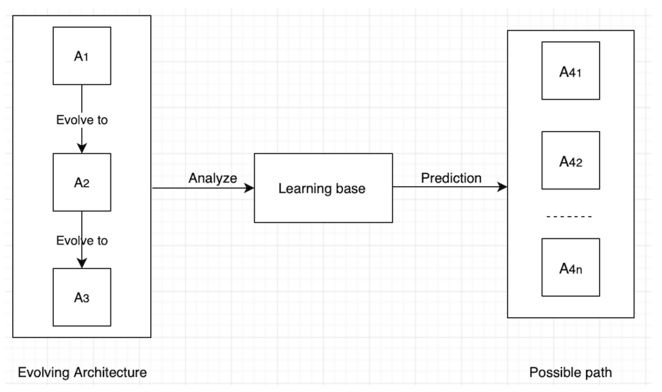
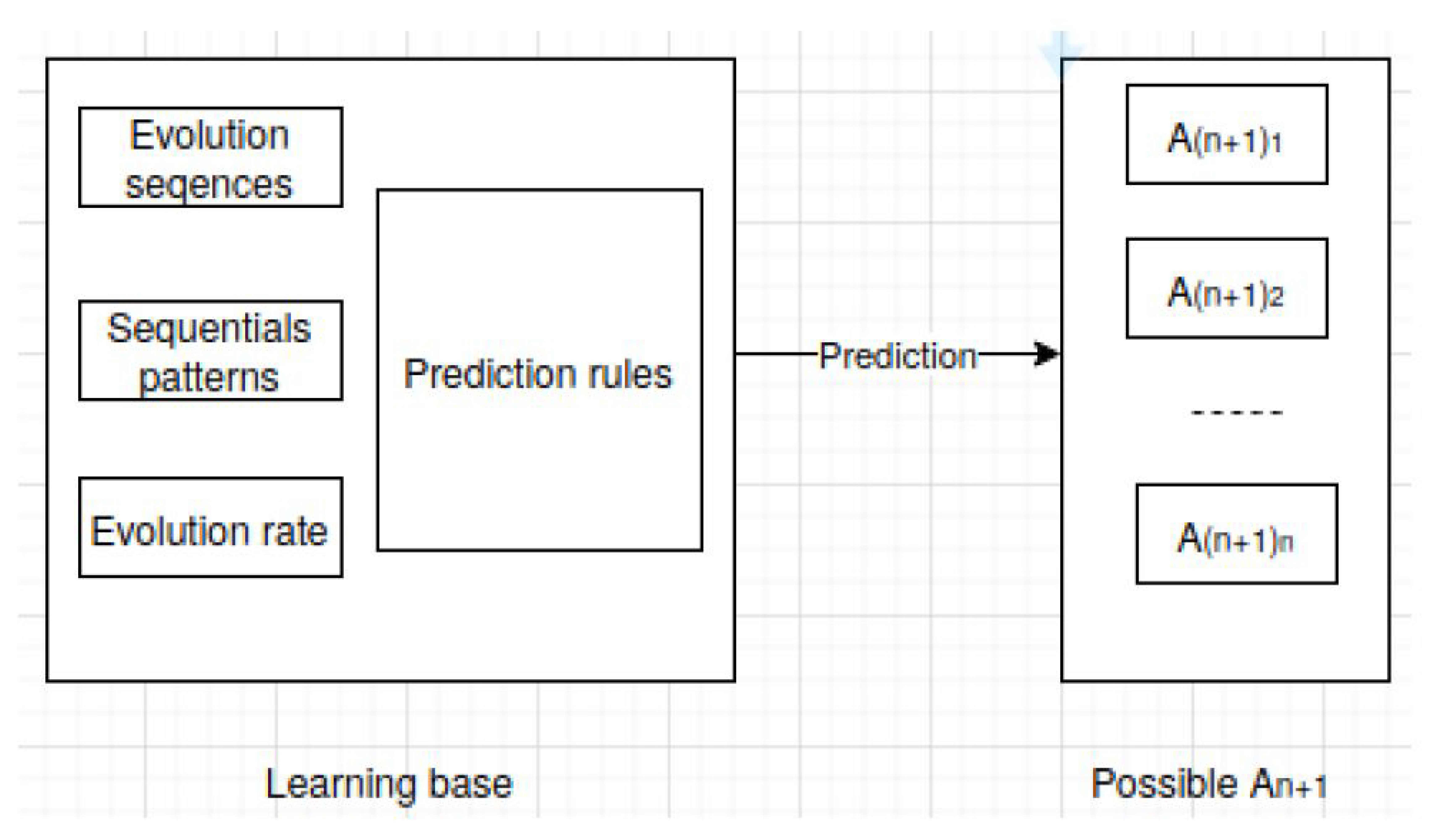
To better explain the approach, we take two examples of the evolution of component-oriented software architecture. In the first example, a trivial architecture evolution is taken, in the second, we take a non-trivial evolution case where an initial architecture evolves to , sequential pattern extraction techniques are applied to predict the possible (, , …, ) as shown in Figure 1 below.
2.2. Examples
For ease of understanding by the reader, we have chosen two simple examples to unfold the models and methodology introduced. The first example presents a simple case of evolution with only operations of creation and modification of architectural elements. The second example, presents a case a little more complex than the first with operations of creation, modification and deletion of architectural elements. The process will be much more complex in the second example. Thus, the two examples reflect the level of difficulty in the process, depending on the number of operations and types of operations combined.
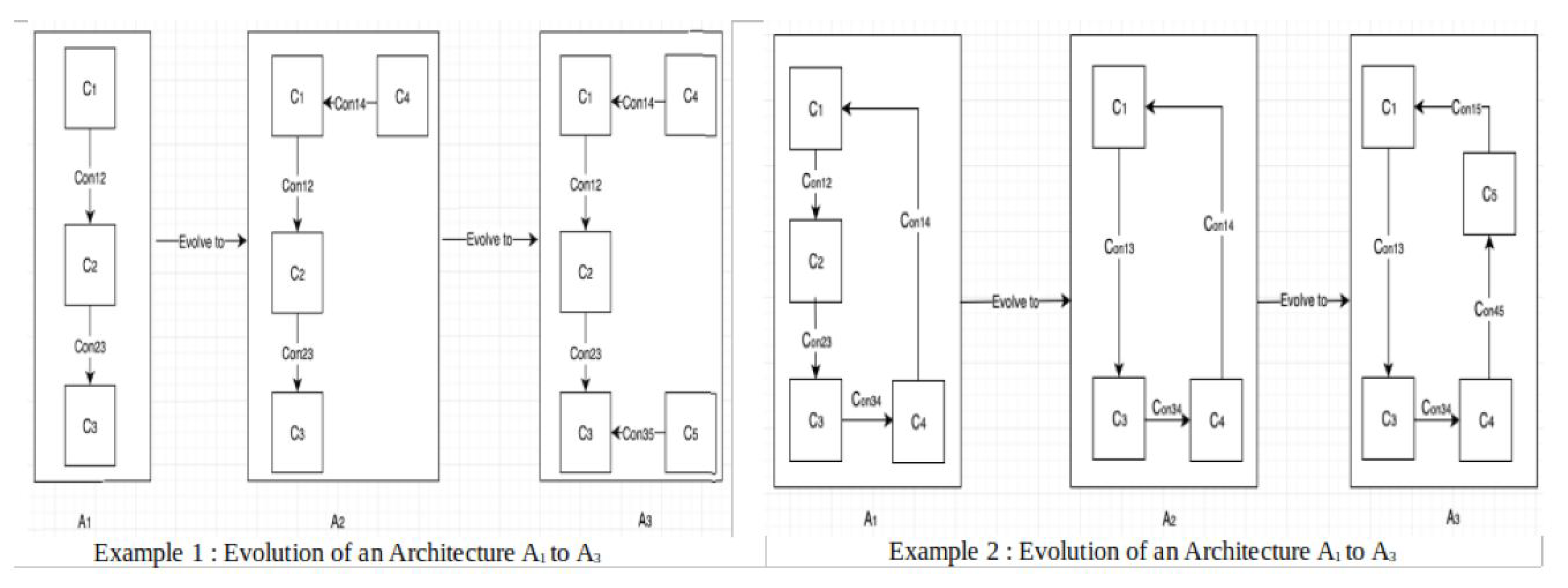
In both examples (Figure 2), we start from a component-oriented architecture evolving to . It is a question of defining a generic model making it possible to predict the possible from the data of evolution from to .
Example 1.
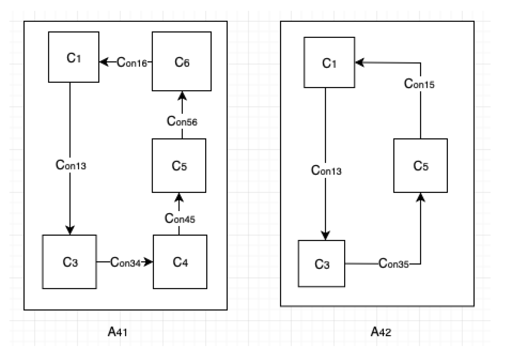
The architecture at the beginning has three components , and . Components are connected by connectors and . The software architect decides to migrate to by creating the component and the connector . In this case study we start with two categories of architectural elements (connector and component).
Example 2.
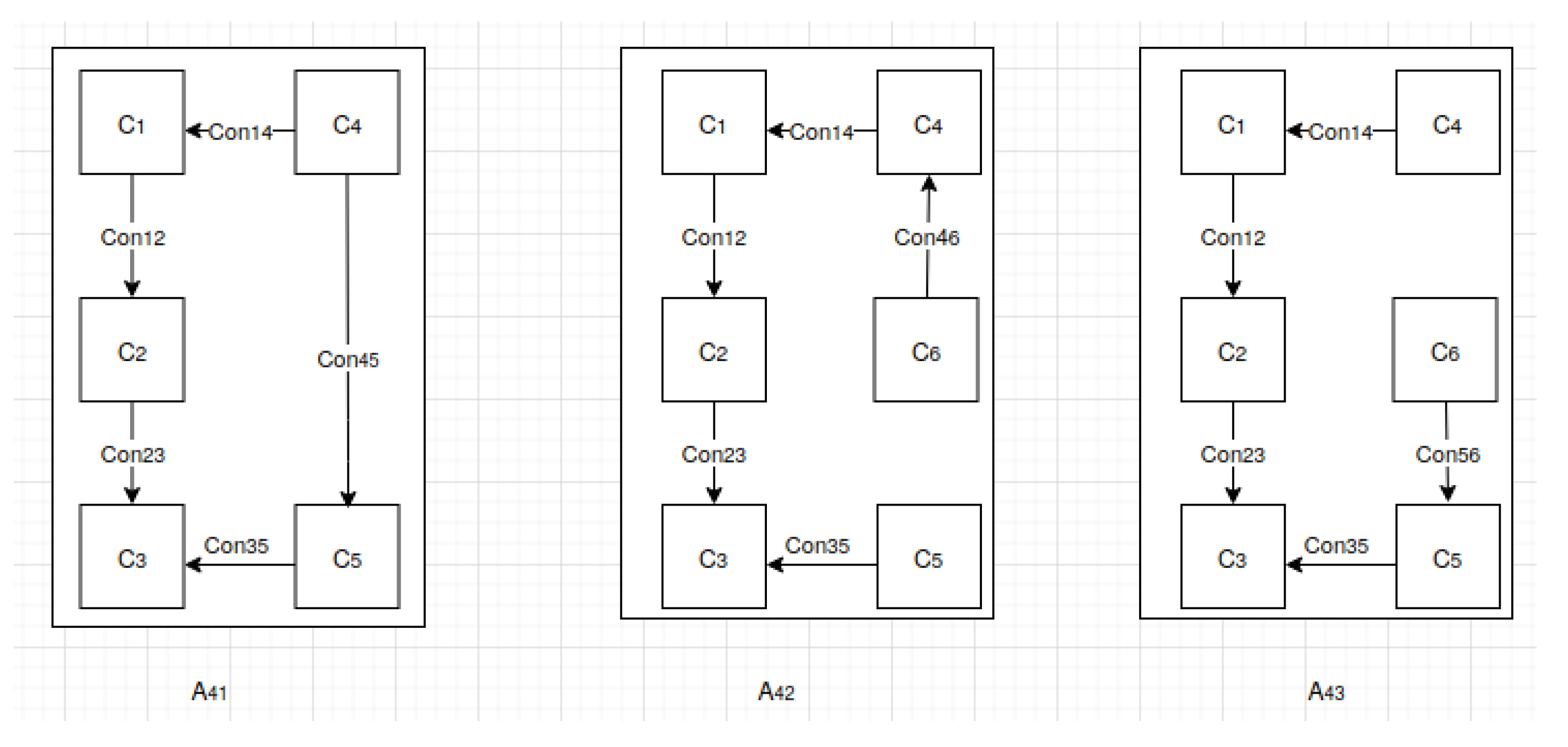
The architecture at the beginning has four components , , and . Components are connected by connectors , , and . The software architect decides to migrate to by deleting the , connectors and the component and creating the connector. has evolved to by removing the connector , creating the component and the connectors and .
In this case study two categories of architectural elements (connector and component) are considered. The evolutions concern the structural aspects of architecture, the behavioural aspects (internal properties) are not taken into account to make the examples more flexible. To achieve our goals, we must first have a database of evolution styles expressed according to the introduced meta-model. For this, a model to represent software architecture evolution is defined in the following section.
3. Evolution Model
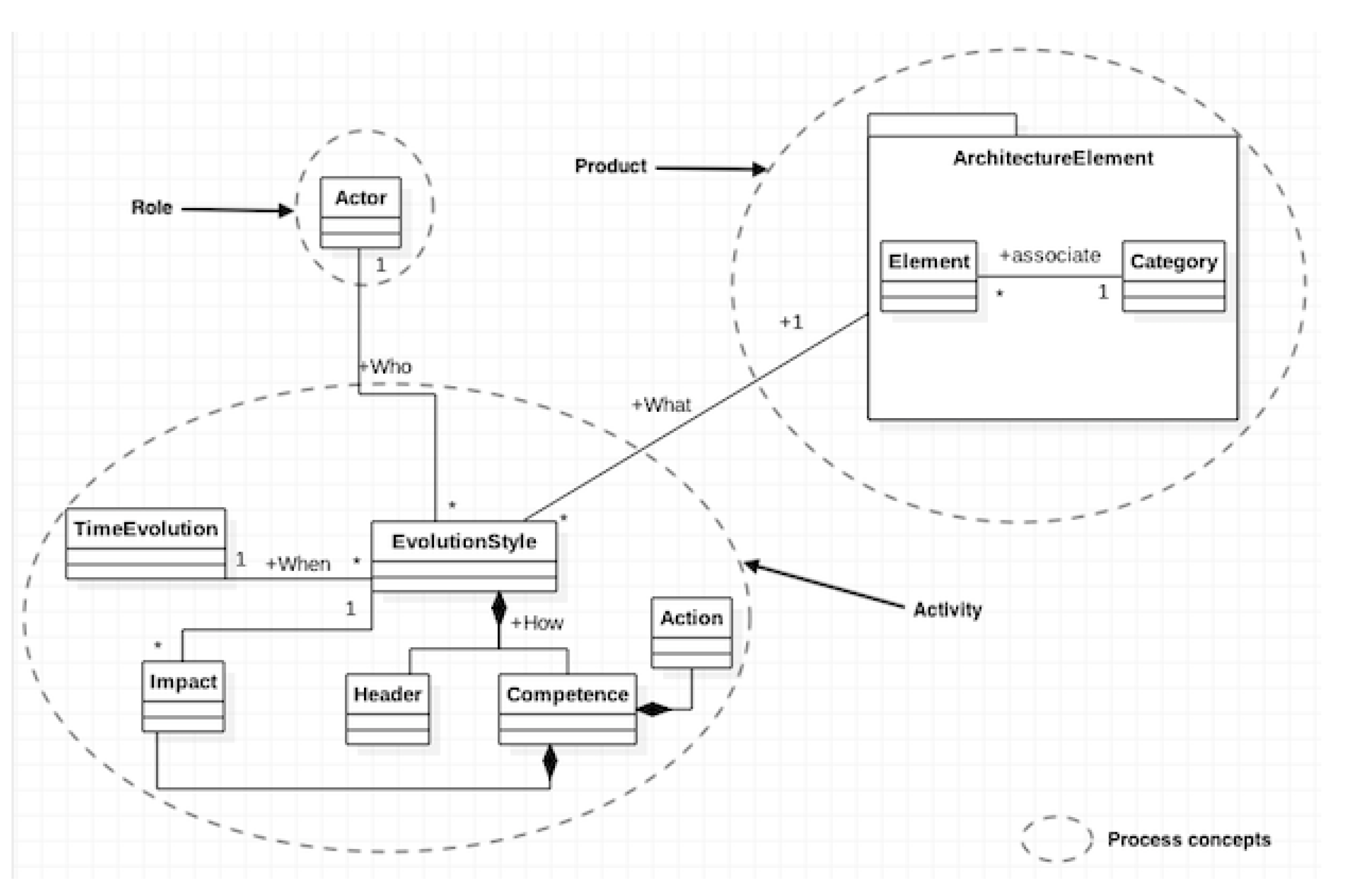
An evolution style captures a characteristic way of evolving all or part of a software architecture. Previously, a meta-model of evolution style was defined [27]. We extend it to define an evolution style as a process (Figure 3) by specifying the role, the architectural element and the operation. Thus, the extended meta-model (Figure 3) answers the following questions: What? (what is evolving?) through the ArchitectureElement package, who? (who did it?) through the Actor concept, when? (when to evolve?) from the TimeEvolution concept and how? (how to make it evolve?) through the concepts Header, Competence, Action ands Impact. All the concepts Header, Competence, Action, Impact define the operation. Through the class diagram in Figure 3 bellow, we highlight the concepts and relations of our model that we call MSAES.
The concept EvolutionStyle is the core of our model, it encapsulates what allows to describe and apply an operation of evolution to an architectural element. It consists of two complementary parts: A header and a competence. The Header class describes the signature of the operation. The competence class is split into Action and Impact. Action is a procedure or function of evolution that focuses on the evolving architectural element. It describes an implementation unit corresponding to the header. The Impact class specifies the evolution styles that will be impacted by the execution of the currently defined style. It allows to establish a relationship between the evolution styles. The Actor concept defines the actor, either a natural person or a program that triggers the operation. The ArchitectureElement package including the evolving element and its category allows to model and reify any significant element of an evolving architecture. If an architectural concept is an instance of this class (in the object-oriented sense), then it becomes possible to associate evolution styles with it. In addition, the Category concept allow to share architectural elements of the same nature in a class. The TimeEvolution class indicates the date on which the evolution operation is performed on the evolving element.
It is the role (defined through the Actor concept), the architectural element and the operation (defined through the Header, Competence, Action and Impact concepts) that allow our meta-model to define an evolution style as a process (Figure 3).
- An instantiation of MSAES on Example 1
- ArchitectureElement: Category of component, Element .
- Action: Creation of component .
- Actor: By Jean.
- TimeEvolution: on 15 December.
- Impact: Creation of connector .
- Header: Creation.
- Each instantiation of the meta-model corresponds to an evolution style.
In the next, the Planning model is presented.
4. Planning Model
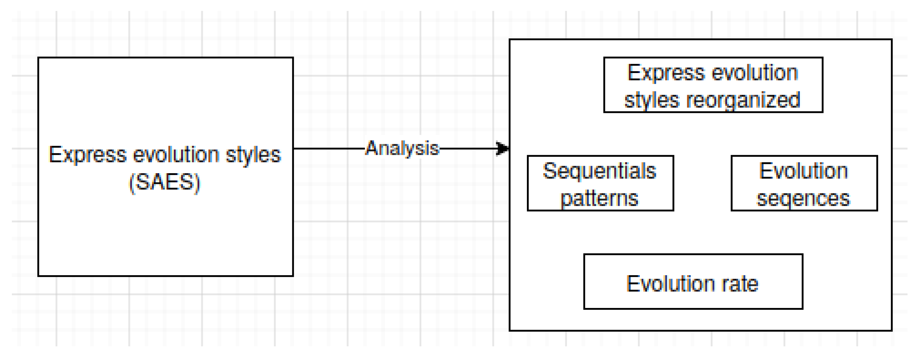
This model is divided into two phases, including The evolution style expression phase, wich uses the previous model (MSAES) and the analysis phase of the expressed evolution styles.
4.1. Expression Phase of Evolution Styles
To easily express evolution styles, we propose a simple expression of evolution style that we call SAES. This expression allows to collect evolution styles of an evolving architecture according to MSAES. SAES specifies the actor, the architectural element, the operation and the evolution date. In MSAES, the operation is defined through the Header and Competence concepts. A Competence is composed of action and impact. The header defined through the Header concept, identifies the evolution operation signature. It is unique, so the operation is replaced by the concept Header. The architectural element is a package including the evolving element and its category, so Element and Category are taken. Figure 4 below represents the formalism.
Finaly, SAES (Figure 4) will allow to name and express one by one all the evolution styles of an evolving architecture to . After expressing all the evolution styles of the evolving architecture with SAES, a large amount of Evolution data is obtained, it can be use to extract the sequential evolution patterns of software architectures, discover the architectural elements change rate and the actors participation rate in evolution operations in order to plan and predict all possible paths towards the architecture.
Below we use SAES to express all evolution styles for evolving to on the two defines examples.
Application to Examples
An architecture structural evolution consists of creation (C), suppression (S) and modification (M) of architectural elements. An architecture can be created (C), suppressed (S), modified (M) or migrated (Mg). The latter results in the creation of a new architecture (advanced version of the previous one). An architecture structural change (M) consists of adding components (), adding connectors (), removing components (), removing connectors () and changing architectural elements. An architectural elements modification consists of adding ports ( and ), deleting ports ( and ) and changing ports () for components and () for connectors.
| Example 1: Evolution style from evolving to | Example 2: Evolution style from evolving to |
| : <Act1, (, Component), , 01-05-2017>. Creation of the component . | : < Act1, (, Component), , 01-05-2017 >. Component creation. |
| : < Act1, (, Component), , 02-05-2017 >. Creation of the component . | : < Act1, (, Component), , 01-05-2017 >. Component creation. |
| : < Act1, (, Connector), , 03-05-2017 >. Creation of the connector . | : < Act1, (, Connector), , 01-05-2017 >. Connector creation. |
| : < Act2, (, Component), , 03-05-2017 >. Creating a port on the component . | : < Act2, (, Component), , 01-05-2017 >. Port creation on . |
| : < Act2, (, Connector), , 03-05-2017 >. Creating a port on the connector . | : < Act2, (, Connector), , 01-05-2017 >. Port creation on . |
| : < Act3, (, Component), , 03-05-2017 >. Modification of the port on the component to connect . | : < Act3, (, Component), , 01-05-2017 >. Port modification on . |
| : < Act3, (, Connector), , 03-05-2017 >. Modification of the port on the connector to connect . | : < Act3, (, Connector), , 01-05-2017 >. Port modification on . |
| : < Act1, (, Component), , 04-05-2017 >. Creation of the component . | : < Act1, (, Component), , 02-05-2017 >. Component creation. |
| : < Act1, (, Connector), , 05-05-2017 >. Creation of the connector . | : < Act1, (, Connector), , 02-05-2017 >. Connector creation. |
| : < Act2, (, Component), , 05-05-2017 >. Creating a port on the component . | : < Act2, (, Component), , 02-05-2017 >. Port creation on . |
| : < Act2, (, Connector), , 05-05-2017 >. Creating a port on the connector . | : < Act2, (, Connector), , 02-05-2017 >. Port creation on . |
| : < Act3, (, Component), , 05-05-2017 >. Modification of the port on the component to connect . | : < Act3, (, Component), , 02-05-2017 >. Port modification on . |
| : < Act3, (, Connector), , 05-05-2017 >. Modification of the port on the connector to connect . | : < Act3, (, Connector), , 02-05-2017 >. Port modification on . |
| : < Act2, (, Component), , 05-05-2017 >. Creating a port on the component . | : < Act2, (, Component), , 02-05-2017 >. Port creation on . |
| : < Act2, (, Connector), , 05-05-2017 >. Creating a port on the connector . | : < Act2, (, Connector), , 02-05-2017 >. Port creation on . |
| : < Act3, (, Component), , 05-05-2017 >. Modification of the port on the component to connect . | : < Act3, (, Component), , 02-05-2017 >. Port modification on . |
| … | … |
| : < Act3, (, Component), , 11-05-2019 >. | : < Act3, (, Connector), , 01-05-2019 >. Port modification on . |
4.2. Analysis Phase of the Expressed Evolution Styles
The expressed evolution styles from the previous phase are analyzed by sequential pattern extraction techniques in order to discover sequential software architecture evolution patterns.
In artificial intelligence, there are 2 main extraction techniques, algorithmic and deep learning. We choose the algorithmic. Referring to the definitions in [13], we define some concepts that we use for the sequential patterns extraction of software architectures evolution.
Evolution sequence: We call an evolution sequence an ordered sequence of evolution style headers applied to a given architectural element or performed by a given actor. The order is established according to the dates of evolution.
Support: The support of an evolution sequence is the percentage of appearance of this sequence in the other evolution sequences.
Sequential pattern: We define sequential pattern of software architectures evolution an ordered sequence of evolution operations carried out in the same order on a defined number of architectural elements. This number defined by the user represents the minimum support of an evolution sequence to be admitted as a sequential pattern.
The sequence length: is the total number of evolution style headers contained in the sequence.
An architectural evolution is an ordered set of evolution operations carried out on the architectural elements (modification of architectural elements) in order to reach a targeted result. An evolution style is a process that describes an evolution operation carried out on a given architectural element during an architectural evolution. Thus, an architectural evolution can be represented by an ordered set of evolution styles. Based on this principle, we use the formalism introduced to extract the sequential evolution patterns of architectures in order to define evolution sequences by architectural element in a category. To do this, we reorganize the styles expressed by defining a table in which we define in column each element of the formalism.
To better explain, let’s apply to the two examples.
Application to the Examples
Inspired by [13], we apply the techniques of sequential patterns extraction to the expressed evolution styles in order to determine the recurrent evolution sequences by category of architectural elements, the rate of change of architectural elements and the actors participation rate in the evolution operations. First, we reorganize the data expressed in a table (Table 1 for example 1, Table 2 for example 2).
Indeed, we are interested in the evolution operations carried out on the architectural elements of the same category during an architectural evolution and the actors associated to these operations. The evolution date allows us to define the operations in sequence by architectural element. After reorganizing the data, we define a second table (Table 3 and Table 4) in which, from the first table defined (Table 1 and Table 2), in a given category we associate with each architectural element the evolution sequence corresponding as in Table 3 and Table 4. The empty sequence () is associated with the element that has not undergone any evolution operation.
| Example 1 | Example 2 |
| ine An interpretation of a line from Table 3 would be: The architectural element after its creation has undergone four evolution operations of header creating component port , component port modification , creating component port and component port modification respectively. From Table 3 we can determine the architectural elements most or least affected by the length of their evolution sequence. The length of the evolution sequence associated with is four, while the length of the sequence associated with is two, we conclude that among the components , , have undergone more evolution operations. We associate with each architecture its sequence of evolution, we note that the architecture has undergone after its creation (C) ten modifications including a component addition , connector addition , etc. before migrating (Mg). | An interpretation of a line from Table 4 would be: The architectural element after its creation has undergone height evolution operations of header creating component port , component port modification , creating component port and five others component port modification respectively. From Table 3 the architectural elements most or least affected can be determined by the length of their evolution sequence. The length of the evolution sequence associated with is six, while the length of the sequence associated with is four, in conclusion, among the components which has the length of eight has undergone more evolution operations. In the same way, the Table 4 associate with each architecture its evolution sequence, so the architecture has undergone after its creation (C) fifteen modifications including a connector suppression , component port modification etc. before migrating (Mg). |
From the tables Table 3 and Table 4, we determine the support of each sequence by category in the following Table 5 for example 1 and Table 6 for example 2, in order to discover the sequential patterns.
We retain as a sequential pattern all evolution sequences with a support value greater than twenty-five percent (25%). This value is arbitrary and can be defined by the user. Table 7 (example 1), Table 8 (example 2) represents the sequential patterns by category of architectural elements.
| Example 1 | Example 2 |
| ine More than twenty-five percent (25%) of components have undergone evolution sequences ( ) and ( ). More than twenty-five percent (25%) of connectors have undergone the sequence ( ). More than twenty-five percent (25%) of architectures have undergone the sequence ( Mg). (Table 7) | More than twenty-five percent (25%) of components have undergone evolution sequences ( ) and ( ). More than twenty-five percent (25%) of connectors have undergone the sequence ( ), ( ) and ( ). More than twenty-five percent (25%) of architectures have undergone the sequence ( Mg), ( Mg) and ( ). (Table 8) |
The sequential evolution patterns of software architectures correspond, in this case, to the evolution sequences or subsequences appearing in the evolution sequences of a number of architectural elements greater than the minimum support specified by the user (k). Thus, to extract them from the Table 3 or Table 4, each sequence must be compared to all the other evolution sequences of the table. If a match is detected its support is incremented. At the end of the table’s path its support is calculated. All the evolution sequences in Table 3 or Table 4 are candidate sequences, i.e., the associated support must be computed in order to extract the software architecture evolution sequential patterns. However, during the table run if an evolution sub-sequence is read in another sequence, this sub-sequence will also be added to the candidate sequences. Its support will also be computed. A sub-sequence ends, begins or is surrounded by the notation () depending on its position respectively start, end or middle of the sequences which contain it. Finally, all the sequences or subsequences having a calculated support greater than k are retained as software architectures evolution sequential patterns. Given the amount of evolution data and processing complexity, it is not easy to extract sequential patterns manually. Thus, an algorithm allowing to extract the sequential patterns from any organized table like the Table 3 or Table 4 whatever the quantity of data is proposed. However, the main challenge in defining sequential pattern extraction algorithms is the high cost of processing due to the high amount of data [23]. Many studies have been carried out in this context, proposing efficient and effective algorithms for the sequential patterns extraction [13,22,23,24,31]. Thus, the objective is centered on the software architecture evolution sequential patterns extraction. Inspired by this work already done to optimize algorithms for extracting sequential patterns, computer algorithms are proposed to extract software architecture evolution sequential patterns from defined data formats (Ex Table 3 or Table 4), compute the evolution rate of an architectural element and the participation rate of an actor in evolution operations.
The Figure 5 below gives a graphic overview of the planning model.
In the next, the methodology used to predict (generate) furture evolution path is presented.
5. Methodology
In order to generate the future evolution paths, we develop a prediction model that uses the output of the planning model and the rules defined for the prediction. Thus, we define two phases including the future path prediction phase and the evaluation phase of proposed paths. In addition, the principles used to extract sequential patterns of software architectures evolution and compute evolution rate are explained, with the overview of some algorithms.
5.1. Future Path Prediction Phase
To propose the possibles (the possibles for this case study) to the architect, a learning and prediction model (Figure 6) is developed. the tables resulting from the analysis carried out in the previous phase are loaded. Figure 6 below provides an overview of the learning and prediction model.
Looking at the two examples:
| Example 1 | Example 2 |
| ine We retain ten possible paths including: Path 1: Creating component , connector between and . Path 2: Creating component , connector between and . Path 3: Creating component , connector between and . Path 4: Creating component , connector between and . Path 5: Creating component , connector between and . Path 6: Creating connector between and . Path 7: Creating connector between and . Path 8: Creating connector between and . Path 9: Creating connector between and . Path 10: Creating connector between and . | We retain eight possible paths including: Path 1: Remove connector , create , and . Path 2: Remove connector and connectors and , create . Path 3: Remove connector and connectors and , create . Path 4: Remove Component and connectors and , create . Path 5: create the component and the connector . Path 6: create the component and the connector . Path 7: create the component and the connector . Path 8: create the component and the connector . |
In order to reduce the possibilities and to retain only the most relevant paths, Some rules are defined for prediction. The rules are dynamic, they can be modified by the architect.
Rule 1
The component connectability notion is defined. A component is said to be connectable if it is possible to connect it to another component via a connector. Indeed, the components contain the ports number property (variable and definable by the architect), if the number of existing connections reaches the component port number, it becomes not connectable. Thus its status can switch to connectable as soon as one of its ports is released following a deletion or a modification. The port number is specified in the component properties. An unconnectable component will not be affected during the prediction.
Rule 2
The architect can define an architectural element that is not sensitive to evolution (Properties, structure and behaviour that make the element non-sensitive). In this case, it will not be affected by future evolution operations.
Rule 3
Architectural elements that have undergone an evolution rate greater than X% (X definable by the architect) are no longer sensitive to evolution.
Rule 4
The architecture must be for example a connected graph.
Rule 5
The expensive elements, whose evolution is expensive are less privileged.
Rule 6
Evolutions involving the architectural elements least affected by previous evolution operations are given priority to evolution.
Let’s Apply Rules to the Examples:
Rules Individual Application
Rule 1: All components have two defined ports, including an incoming port and an outgoing port, you cannot go beyond these two connections on a component.
| Example 1 | Example 2 |
| ine Path 1, 2, 3, 6, 7, 9 and 10 will be totally excluded for rule 1 violation. The possibilities remain paths 4, 5 and 8. | Paths 5, 6, 7 and 8 will be totally excluded for rule 1 violation. The possibilities remain paths 1, 2, 3 and 4. |
Rule 2: The component is defined not sensitive to evolution.
| Example 1 | Example 2 |
| ine Path 2 and 7 will be totally excluded for rule 2 violation. The possibilities remain paths 1, 3, 4, 5, 6, 8, 9 and 10. | only Path 4 will be excluded for rule 2 violation. The other paths remain possible alternatives. |
Rule 3: X (maximum architectural element change rate) is set at seventy-five percent (75%). For this, refer to the evolution rate by architectural element. It does not take effect, because no element has reached the indicated threshold.
Rule 4: For example, and are defined as expensive items.
| Example 1 | Example 2 |
| ine Paths 2, 3, 7 and 10 will be totally excluded for rule 4 violation. The possibilities remain paths 1, 4, 5, 6, 8 and 9. | Paths 3 and 4 will be totally excluded for rule 4 violation. The possibilities remain paths 1, 2, 5, 6, 7 and 8. |
Rule 5: Referring to the evolution rate, components and have a lower priority for evolution.
| Example 1 | Example 2 |
| ine Paths 1, 2, 6, 7 and 9 will be totally excluded for above rule violation. The possibilities remain paths 3, 4, 5, 8 and 10. | Paths 4 will be totally excluded for above rule violation. The possibilities remain paths 1, 2, 3, 5, 6, 7 and 8. |
Rules Together Application:
Thus, the paths not violating any of the rules of all the categories involved are retained.
- -
- Rules 1–3:
Example 1 Example 2 ine Paths 4, 5 and 8 are retained. Paths 1, 2 and 3 are retained.
- -
- Rules 1, 5 and 6:
Example 1 Example 2 ine Paths 4, 5 and 8 are retained. Paths 1 and 2 are retained.
- -
- Rules 1 to 6:
Example 1 Example 2 ine Paths 4, 5 and 8 are retained. Paths 1 and 2 are retained.
Whatever order you choose (Rule 1 and Rule 2 or Rule 2 and Rule 1), the same paths retained is obtained.
For this case study, all difined rules apply together are considered. The paths chosen for each example are highlight:
| Example 1 | Example 2 |
ine
|
5.2. Evaluation Phase of Proposed Paths
This evaluation is based on Table 7 and Table 8, the sequence associated with the architecture being migrated is compared to the sequential patterns associated with the architecture discovered (Table 7 and Table 8), if the sequence is identical to one of the sequential patterns discovered the weight one (1) is associated with the possibility otherwise the zero weight (0). Otherwise if it has identical parts to a sub-sequence pattern, the half weight (0.5) is associated with it. In table (Table 9 for example 1 and Table 10 for example 2), the proposed paths evaluation is presented.
By considering that the priorities given to the different rules could give a better quality of results. This choice will ultimately be left to the architect.
In addition, the evolution sequences by actor (Table 4) and the actors participation rate calculation in the evolution operation allow to plan the future evolution operations proposed. Indeed, for each path, the skills (actors) that can intervene can be proposed.
Table 11 and Table 12 give a global overview of the other results obtained at the end of example 2 in addition to the other defined tables.
In the next, The principles adapted for software architecture evolution sequentials patterns extraction and architectural elements evolution rate computation are explained, with the overview of some algorithms.
5.3. Principle to Extract Sequential Patterns of Software Architectures Evolution
A first functionis defined, which starting from the Table 1, associates with each architectural element, the corresponding evolution sequence. The function named Sequence (Algorithm 1), retrieves the table (Table 1) sorted on the Category, TimeEvolution and Element columns and associates with each architectural element the corresponding evolution sequence. It provides as an output an equivalent of Table 2. The second function named SequenceSupport (Algorithm 2) allows to compute and associate to each candidate sequence its support, it takes as input the candidate sequences defined from Table 2 (output of the previous function), then computes and associates to each sequence its total number of appearance among all the other candidate sequences. It provides as an output a table that associates each candidate sequence with its total appearances number. The SequentialPattern function (Algorithm 3) returns sequential patterns by category of architectural elements with k support provided as a parameter. For example, if a k equal to twenty-five percent is taken, the sequential patterns will correspond to all the evolution sequences or sub-sequences appearing in the evolution sequences of more than twenty-five percent of architectural elements in the same category. It takes as input the output of the previous function, computes and associates to each candidate sequence its support in percentage and compares it to the minimum support k provided in parameter. If a superiority is read, the current sequence is stored in the sequential pattern table. At the end of the process, it provides this sequential pattern table which contains all the sequences with a support higher than the k provided.
| Algorithm 1 Sequence |
|
| Algorithm 2 Sequence Support |
|
| Algorithm 3 Sequentials Patterns |
|
5.4. Principle for Calculating the Rate of Change of Architectural Elements
The PercentageEvolution function (Algorithm 4) takes as input any table similar to Table 2 associated with Table 1 that contains all the evolution operations performed. It associates to each architectural element, its evolution rate by multiplying the evolution sequence size associated with the element by hundred then dividing the result by n (the size of Table 1 or the total number of evolution styles involved in the search for sequential patterns). As an output, the algorithm provides a two-column table where, to each architectural element is associated its evolution rate or to each actor its participation rate in evolution operations.
| Algorithm 4 PurcentageEvolution |
|
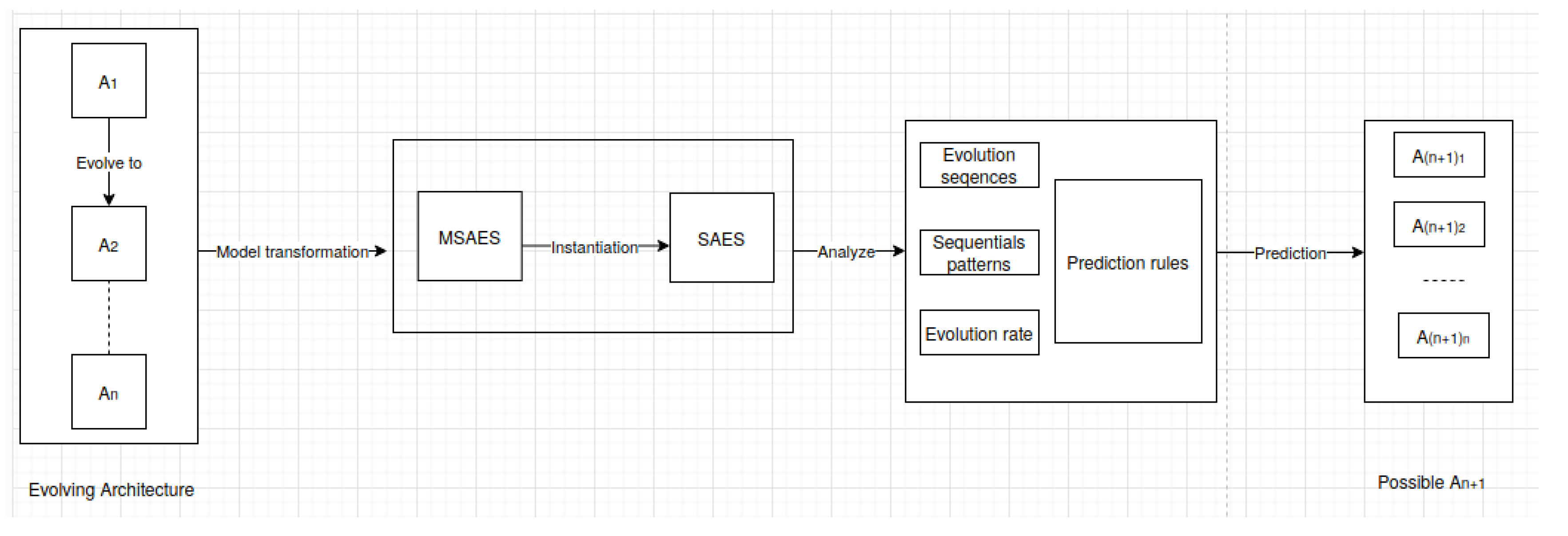
In Figure 9 below, we give a graphical overview of the models and the methodology presented with the transition flow between the models.
6. Discussion and Conclusions
In the literature, we found two works similar to that proposed in this paper. These are [29,30]. Even if the two works and ours propose a solution to automate the software architecture evolution process, there is still a big difference with respect to the final objectives and the methodologies used to achieve the objectives. According to [29], the user must specify the desired types of evolution and introduce the initial architecture (specified in xADL). Then the evolution alternatives are generated with a graph transformation tool. According to [30], the user must specify the initial architecture and the target architecture. Then, using an automatic planner the path (in terms of transition architectures) by which the initial architecture can evolve towards the target architecture is generated. While, we propose in this paper an approach based on Oussalah et al. evolution style approach and sequential pattern extraction techniques to learn through previous evolutions of the evolving architecture, to predict and plan possible future evolution paths. The user only has to provide the previous evolution data, by learning the system generates all the possible evolution paths. In addition, we provide a means of evaluating the different evolution paths generated through the learning of previous evolution data to support the architect in the choice of the best path.
At this stage of the work, the user must provide the system with all previous data on the evolution of the architecture, from its initial state to its latest version according to SAES. This can be tedious or even impossible depending on the amount of evolution data. Thus, to make it easier for the user, a model transformation allowing the automatic translation of the architecture evolution graphical representation (e.g., Figure 2) to the evolution styles expressed by the SAES formalism is required.
In this paper, a solution for predicting and planning future evolution paths of software architecture is presented. It is applied, tested and validated on two examples of trivial and non-trivial component-oriented software architecture evolution. The two examples, cases of trivial and non-trivial evolution, allow us to theorically validate our model on component-oriented software architectures. However, further work is needed to definitively and completely validate the model and extend it to other types of architectures.
In the near future, the validity of the model on other types of architectures will be evaluated. An implementation of the model with a programming language is envisaged, with the possibility of a model transformation to move from a graphical representation of an architecture evolution using any xADL to our formalisms.
Author Contributions
Methodology, K.D. and M.C.O.; supervision, M.C.O. and J.K.; validation, M.C.O.; writing—original draft preparation, all authors; writing—review and editing, all authors. All authors have read and agreed to the published version of the manuscript.
Funding
This research received no external funding.
Conflicts of Interest
The authors declare no conflict of interest.
References
- Bhattacharya, P.; Iliofotou, M.; Neamtiu, I.; Faloutsos, M. Graph-based analysis and prediction for software evolution. In Proceedings of the 2012 34th International Conference on Software Engineering (ICSE), Zurich, Switzerland, 2–9 June 2012; pp. 419–429. [Google Scholar]
- Goulão, M.; Fonte, N.; Wermelinger, M.; e Abreu, F.B. Software evolution prediction using seasonal time analysis: A comparative study. 2012 16th European Conference on Software Maintenance and Reengineering? In Proceedings of the16th European Conference on Software Maintenance and Reengineering, CSMR 2012, Szeged, Hungary, 27–30 March 2012; pp. 213–222. [Google Scholar]
- Herbold, V. Mining Developer Dynamics for Agent-Based Simulation of Software Evolution. Ph.D. Thesis, University of Göttingen, Göttingen, Germany, 2019. [Google Scholar]
- Jaafar, F.; Lozano, A.; Guéhéneuc, Y.; Mens, K. Analyzing software evolution and quality by extracting Asynchrony change patterns. J. Syst. Softw. 2017, 131, 311–322. [Google Scholar] [CrossRef]
- Gasmallah, N.; Amirat, A.; Oussalah, M.; Seridi-Bouchelaghem, H. Developing an evolution software architecture framework based on six dimensions. Int. J. Simul. Process. Model. 2019, 14, 325–337. [Google Scholar] [CrossRef]
- Hassan, A.; Oussalah, M.C. Evolution Styles: Multi-View/Multi-Level Model for Software Architecture Evolution. JSW 2018, 13, 146–154. [Google Scholar] [CrossRef]
- Hassan, A.; Oussalah, M. Meta-Evolution Style for Software Architecture Evolution. In SOFSEM 2016: Theory and Practice of Computer Science—42nd International Conference on Current Trends in Theory and Practice of Computer Science, Harrachov, Czech Republic, 23–28 January 2016; Freivalds, R.M., Engels, G., Catania, B., Eds.; Lecture Notes in Computer Science; Springer: Berlin/Heidelberg, Germany, 2016; Volume 9587, pp. 478–489. [Google Scholar] [CrossRef]
- Filho, J.W.; de Figueiredo Carneiro, G.; Maciel, R.S.P. A Systematic Mapping on Visual Solutions to Support the Comprehension of Software Architecture Evolution. In Proceedings of the 25th International DMS Conference on Visualization and Visual Languages, DMSVIVA 2019, Hotel Tivoli, Lisbon, Portugal, 8–9 July 2019; Joseph, J.P., Jr., Ed.; KSI Research Inc. and Knowledge Systems Institute Graduate School: Skokie, IL, USA, 2019; pp. 63–82. [Google Scholar] [CrossRef]
- Smeda, A.; Oussalah, M.; Khammaci, T. Madl: Meta architecture description language. In Proceedings of the Third ACIS International Conference on Software Engineering, Research, Management and Applications (SERA 2005), Mt. Pleasant, MI, USA, 11–13 August 2005; pp. 152–159. [Google Scholar]
- Magee, J.; Kramer, J. Dynamic structure in software architectures. In ACM SIGSOFT Software Engineering Notes; ACM: New York, NY, USA, 1996; Volume 21, pp. 3–14. [Google Scholar]
- Dashofy, E.M.; Van der Hoek, A.; Taylor, R.N. A highly-extensible, XML-based architecture description language. In Proceedings of the 2001 Working IEEE / IFIP Conference on Software Architecture (WICSA 2001), Amsterdam, The Netherlands, 28–31 August 2001; pp. 103–112. [Google Scholar]
- Cuesta, C.E.; Navarro, E.; Perry, D.E.; Roda, C. Evolution styles: Using architectural knowledge as an evolution driver. J. Softw. Evol. Process 2013, 25, 957–980. [Google Scholar] [CrossRef]
- Agrawal, R.; Srikant, R. Mining Sequential Patterns. In Proceedings of the Eleventh International Conference on Data Engineering, Taipei, Taiwan, 6–10 March 1995; pp. 3–14. [Google Scholar]
- Wu, Y.H.; Chen, A.L. Prediction of web page accesses by proxy server log. World Wide Web 2002, 5, 67–88. [Google Scholar] [CrossRef]
- Hsu, J.L.; Liu, C.C.; Chen, A.L. Discovering nontrivial repeating patterns in music data. IEEE Trans. Multimed. 2001, 3, 311–325. [Google Scholar]
- Xie, T.; Thummalapenta, S.; Lo, D.; Liu, C. Data mining for software engineering. Computer 2009, 42, 55–62. [Google Scholar] [CrossRef]
- Amaral, J.N.; Jocksch, A.P.; Mitran, M. Mining Sequential Patterns in Weighted Directed Graphs. U.S. Patent 8,683,423, 1 April 2014. [Google Scholar]
- Ahmad, A.; Jamshidi, P.; Arshad, M.; Pahl, C. Graph-based implicit knowledge discovery from architecture change logs. In Proceedings of the 2012 Joint Working IEEE/IFIP Conference on Software Architecture and European Conference on Software Architecture, WICSA/ECSA 2012, Helsinki, Finland, 20–24 August 2012; pp. 116–123. [Google Scholar]
- Bogorny, V.; Avancini, H.; de Paula, B.C.; Kuplich, C.R.; Alvares, L.O. Weka-STPM: A Software Architecture and Prototype for Semantic Trajectory Data Mining and Visualization. Trans. GIS 2011, 15, 227–248. [Google Scholar] [CrossRef]
- Javed, M.; Abgaz, Y.M.; Pahl, C. Graph-Based Discovery of Ontology Change Patterns. In Proceedings of the International Semantic Web Conference (ISWC) Workshops: Joint Workshop on Knowledge Evolution and Ontology Dynamics (EvoDyn), Bonn, Germany, 24 October 2011. [Google Scholar]
- Wright, A.P.; Wright, A.T.; McCoy, A.B.; Sittig, D.F. The Use of Sequential Pattern Mining to Predict Next Prescribed Medications. J. Biomed. Inform. 2015, 53, 73–80. [Google Scholar] [CrossRef] [PubMed] [Green Version]
- Srikant, R.; Agrawal, R. Mining sequential patterns: Generalizations and performance improvements. In Proceedings of the International Conference on Extending Database Technology; Springer: Berlin/Heidelberg, Germany, 1996; pp. 1–17. [Google Scholar]
- Chiu, D.Y.; Wu, Y.H.; Chen, A.L. An efficient algorithm for mining frequent sequences by a new strategy without support counting. In Proceedings of the 20th International Conference on Data Engineering, ICDE 2004, Boston, MA, USA, 30 March–2 April 2004; pp. 375–386. [Google Scholar]
- Ziembiński, R. Algorithms for context based sequential pattern mining. Fundam. Inform. 2007, 76, 495–510. [Google Scholar]
- Alkan, O.K.; Karagoz, P. CRoM and HuspExt: Improving efficiency of high utility sequential pattern extraction. In Proceedings of the 32nd IEEE International Conference on Data Engineering, ICDE 2016, Helsinki, Finland, 16–20 May 2016; pp. 1472–1473. [Google Scholar] [CrossRef]
- Mooney, C.; Roddick, J.F. Sequential pattern mining—Approaches and algorithms. ACM Comput. Surv. 2013, 45, 19:1–19:39. [Google Scholar] [CrossRef]
- Oussalah, M.C.; Le Goaer, O.; Tamzalit, D.; Seriai, A. Evolution Shelf: Exploiting Evolution Styles within Software Architectures. In Proceedings of the Twentieth International Conference on Software Engineering & Knowledge Engineering (SEKE’2008), San Francisco, CA, USA, 1–3 July 2008; pp. 387–392. [Google Scholar]
- Garlan, D. Evolution Styles-Formal Foundations and Tool Support for Software Architecture Evolution; School of Computer Science, Carnegie Mellon University: Pittsburgh, PA, USA, 2008; p. 650. [Google Scholar]
- Ciraci, S.; Sozer, H.; Aksit, M. Guiding architects in selecting architectural evolution alternatives. In Proceedings of the European Conference on Software Architecture, Essen, Germany, 13–16 September 2011; pp. 252–260. [Google Scholar]
- Barnes, J.M.; Pandey, A.; Garlan, D. Automated planning for software architecture evolution. In Proceedings of the 2013 28th IEEE/ACM International Conference on Automated Software Engineering, ASE 2013, Silicon Valley, CA, USA, 11–15 November 2013; pp. 213–223. [Google Scholar]
- Mahajan, S.; Pawar, P.; Reshamwala, A. Performance Analysis of Sequential Pattern Mining Algorithms on Large Dense Datasets. Int. J. Appl. Innov. Eng. Manag. 2014, 3, 345–351. [Google Scholar]
Figure 1.
Goal.

Figure 2.
The two examples.

Figure 3.
Software architecture evolution style meta-modèle (MSAES).

Figure 4.
SAES.

Figure 5.
Planning model.

Figure 6.
Learning and prediction model.

Figure 7.
Example 1: Possibilities.

Figure 8.
Example 2: Possibilities.

Figure 9.
Graphical overview.


Table 1.
Example 1: The evolution styles of architecture to reorganised.
| Architecture Evolution | Style Name | Actor | Element | Category | Header | TimeEvolution |
|---|---|---|---|---|---|---|
| Act1 | Component | 01-05-2017 | ||||
| Act1 | Component | 02-05-2017 | ||||
| Act1 | Connector | 03-05-2017 | ||||
| Act2 | Component | 03-05-2017 | ||||
| Act2 | Connector | 03-05-2017 | ||||
| Act3 | Component | 03-05-2017 | ||||
| Act3 | Connector | 03-05-2017 | ||||
| Act2 | Component | 03-05-2017 | ||||
| Initial | Act2 | connector | 03-05-2017 | |||
| architecture | Act3 | Component | 03-05-2017 | |||
| creation | Act3 | connector | 03-05-2017 | |||
| Act1 | Component | 04-05-2017 | ||||
| Act1 | connector | 05-05-2017 | ||||
| Act2 | Component | 05-05-2017 | ||||
| Act2 | Connector | 05-05-2017 | ||||
| Act3 | Component | 05-05-2017 | ||||
| Act3 | Connector | 05-05-2017 | ||||
| Act2 | Component | 05-05-2017 | ||||
| Act2 | Connector | 05-05-2017 | ||||
| Act3 | Component | 05-05-2017 | ||||
| Act3 | Connector | 05-05-2017 | ||||
| Act1 | Component | 06-05-2018 | ||||
| Act1 | Connector | 07-05-2018 | ||||
| Act2 | Component | 07-05-2018 | ||||
| Act2 | Connector | 07-05-2018 | ||||
| Act3 | Component | 07-05-2018 | ||||
| Act3 | Connector | 07-05-2018 | ||||
| Act2 | Component | 07-05-2018 | ||||
| Act2 | Connector | 07-05-2018 | ||||
| Act3 | Component | 07-05-2018 | ||||
| Act3 | Connector | 07-05-2018 | ||||
| Act1 | Component | 10-05-2019 | ||||
| Act1 | Connector | 11-05-2019 | ||||
| Act2 | Component | 11-05-2019 | ||||
| Act2 | Connector | 11-05-2019 | ||||
| Act3 | Component | 11-05-2019 | ||||
| Act3 | Connector | 11-05-2019 | ||||
| Act2 | Component | 11-05-2019 | ||||
| Act2 | Connector | 11-05-2019 | ||||
| Act3 | Component | 11-05-2019 | ||||
| Act3 | Connector | 11-05-2019 |
Table 2.
Example 2: The evolution styles of architecture to reorganised.
| Architecture Evolution | Style Name | Actor | Element | Category | Header | TimeEvolution |
|---|---|---|---|---|---|---|
| Act1 | Component | 01-05-2017 | ||||
| Act1 | Component | 02-05-2017 | ||||
| Act1 | Connector | 03-05-2017 | ||||
| Act2 | Component | 03-05-2017 | ||||
| Act2 | Connector | 03-05-2017 | ||||
| Act3 | Component | 03-05-2017 | ||||
| Act3 | Connector | 03-05-2017 | ||||
| Act2 | Component | 03-05-2017 | ||||
| Initial | Act2 | connector | 03-05-2017 | |||
| architecture | Act3 | Component | 03-05-2017 | |||
| creation | Act3 | connector | 03-05-2017 | |||
| Act1 | Component | 04-05-2017 | ||||
| Act1 | connector | 05-05-2017 | ||||
| Act2 | Component | 05-05-2017 | ||||
| Act2 | Connector | 05-05-2017 | ||||
| … | … | … | … | … | … | |
| Act4 | Connector | 01-06-2018 | ||||
| Act4 | Component | 01-06-2018 | ||||
| Act4 | Component | 01-06-2018 | ||||
| Act4 | Connector | 02-06-2018 | ||||
| Act4 | Component | 02-06-2018 | ||||
| Act4 | Component | 02-06-2018 | ||||
| Act4 | Component | 03-06-2018 | ||||
| Act1 | Connector | 03-06-2018 | ||||
| Act2 | Connector | 03-06-2018 | ||||
| … | … | … | … | … | … | |
| Act4 | Connector | 01-04-2019 | ||||
| Act4 | Component | 01-04-2019 | ||||
| Act4 | Component | 01-04-2019 | ||||
| Act1 | Component | 10-04-2019 | ||||
| Act1 | Connector | 10-04-2019 | ||||
| Act2 | Connector | 11-04-2019 | ||||
| Act3 | Component | 11-04-2019 | ||||
| Act3 | Connector | 11-04-2019 | ||||
| Act2 | Component | 11-04-2019 | ||||
| … | … | … | … | … | … |
Table 3.
Example 1: Evolution sequence by architectural element and category.
| Category | Element | Evolution Sequence |
|---|---|---|
| ( ) | ||
| ( ) | ||
| Component | ( ) | |
| ( ) | ||
| ( ) | ||
| ( ) | ||
| Connector | ( ) | |
| ( ) | ||
| ( ) | ||
| Architecture | ( Mg) | |
| ( Mg) |
Table 4.
Example 2: Evolution sequence by element in category.
| Category | Element | Evolution Sequence |
|---|---|---|
| ( ) | ||
| ( ) | ||
| Component | ( ) | |
| ( ) | ||
| ( ) | ||
| ( ) | ||
| ( ) | ||
| ( ) | ||
| Connector | ( ) | |
| ( ) | ||
| ( ) | ||
| ( ) | ||
| ( Mg) | ||
| Architecture | ( Mg) | |
| () | ||
| Act1 | ( ) | |
| Act2 | ( ) | |
| Actor | Act3 | ( ) |
| Act4 | ( ) |
Table 5.
Example 1: Support by architectural element and category.
| Category | Evolution Sequence | Support |
|---|---|---|
| Architecture | ( Mg) | 66.6% |
| Component | ( ) | 60% |
| ( ) | 100% | |
| Connector | ( ) | 100% |
Table 6.
Example 2: Support by sequence in category.
| Category | Evolution Sequence | Support |
|---|---|---|
| ( Mg) | 33.33% | |
| Architecture | ( Mg) | 33.33% |
| ( ) | 66.66% | |
| ( ) | 66.66% | |
| ( ) | 20% | |
| ( ) | 20% | |
| ( ) | 20% | |
| Component | ( ) | 20% |
| ( ) | 80% | |
| ( ) | 100% | |
| ( ) | 42.86% | |
| Connector | ( ) | 57.14% |
| ( ) | 100% |
Table 7.
Example 1: Sequential pattern by category of architectural elements.
| Category | Sequential Pattern >25% |
|---|---|
| Architecture | ( Mg) |
| Component | ( ) |
| ( ) | |
| Connector | ( ) |
Table 8.
Example 2: Sequential pattern by category of architectural elements.
| Category | Sequential Pattern >25% |
|---|---|
| ( Mg) | |
| Architecture | ( Mg) |
| ( ) | |
| ( ) | |
| Component | ( ) |
| ( ) | |
| ( ) | |
| Connector | ( ) |
| ( ) |
Table 9.
Example 1: Evaluation.
| Possibilities | Evolution Sequence | Weight |
|---|---|---|
| ( Mg) | 1 | |
| ( Mg) | 1 | |
| ( Mg) | 0.5 |
Table 10.
Example 2: Evaluation.
| Possibilities | Evolution Sequence | Weight |
|---|---|---|
| ( Mg) | 1 | |
| ( Mg) | 1 |
Table 11.
Example 1: Other results.
| Category | Result |
|---|---|
| Architectural elements most affected | , , , , , , |
| Architectural elements less affected | and |
| The selected architecture | or |
| The most active actors | Act2 and Act3 |
| The least active actors | Act1 |
Table 12.
Example 2: Other results.
| Category | Result |
|---|---|
| Architectural elements most affected | , , , , , , |
| Architectural elements less affected | , , , , |
| The selected architecture | or |
| The most active actors | Act2 and Act3 |
| The least active actors | Act1 |
© 2020 by the authors. Licensee MDPI, Basel, Switzerland. This article is an open access article distributed under the terms and conditions of the Creative Commons Attribution (CC BY) license (http://creativecommons.org/licenses/by/4.0/).
Share and Cite
MDPI and ACS Style
Djibo, K.; Oussalah, M.C.; Konate, J. Modelling and Planning Evolution Styles in Software Architecture. Modelling 2020, 1, 53-76. https://0-doi-org.brum.beds.ac.uk/10.3390/modelling1010004
AMA Style
Djibo K, Oussalah MC, Konate J. Modelling and Planning Evolution Styles in Software Architecture. Modelling. 2020; 1(1):53-76. https://0-doi-org.brum.beds.ac.uk/10.3390/modelling1010004
Chicago/Turabian StyleDjibo, Kadidiatou, Mourad Chabane Oussalah, and Jacqueline Konate. 2020. "Modelling and Planning Evolution Styles in Software Architecture" Modelling 1, no. 1: 53-76. https://0-doi-org.brum.beds.ac.uk/10.3390/modelling1010004