Stochastic Earthmoving Fleet Arrangement Optimization Considering Project Duration and Cost


1
Department of Civil and Environmental Engineering, University of Alberta, Edmonton, AB T6G 1H9, Canada
2
Department of Civil and Environmental Engineering, University of Central Florida, Orlando, FL 32816, USA
3
Building Construction Science Department, College of Architecture, Art and Design, Mississippi State University, P.O. Box 6222, Starkville, MS 39762, USA
*
Author to whom correspondence should be addressed.
Modelling 2020, 1(2), 156-174; https://0-doi-org.brum.beds.ac.uk/10.3390/modelling1020010
Submission received: 14 September 2020
/
Revised: 2 November 2020
/
Accepted: 3 November 2020
/
Published: 7 November 2020
(This article belongs to the Special Issue Feature Papers of Modelling)
Abstract
:Earthmoving is one of the main processes involved in heavy construction and mining projects. It requires a significant share of the project budget and can dictate its overall success. Earthmoving related activities have a stochastic nature that affects the project cost and duration. In common practice, the equipment required for a project is selected using average operating cycles, neglecting the stochastic nature of operations and equipment. Ultimately this can lead to rough estimates and poor results in meeting the projects’ objectives. This research aims to provide a decision-support tool for earthmoving operations and achieve the best arrangement of equipment based on project objectives and equipment specifications by utilizing historical data. Operation simulation is identified as an efficient technique to model and analyze the stochastic aspects of the cost and duration of earthmoving operations in construction projects. Therefore, two simulation models—namely the Decision-Support Model and the Estimation Model, have been developed in the Symphony.net modeling environment to address the industry needs. The Decision-Support Model provides the best arrangement of equipment to maximize global resource utilization. In contrast, the Estimation Model captures more of the project details and compares various equipment arrangements. In this paper, these models are created, and the modeling logic is validated through a case study employing a real-world earthmoving project that demonstrates the model’s capabilities. The decision support model showed promising results in determining the optimized fleet selection when considering equipment and shift variations, and the cost model helped better quantifying the impact of the decision on the cost and profit of the project. This modeling approach can be reproduced by others in any case of interest to gain optimal fleet management.
1. Introduction
In terms of scope and detail, heavy construction projects can be categorized as some of the largest industries in the world. Earthmoving is an integral part of heavy construction projects and requires substantial financial investments in the purchasing or renting of heavy equipment, in addition to signficant operational and maintenance costs [1]. The optimum employment of equipment is a vital responsibility for the project management team, and, if done properly, can lead to considerable savings in both the time and cost of earthmoving operations.
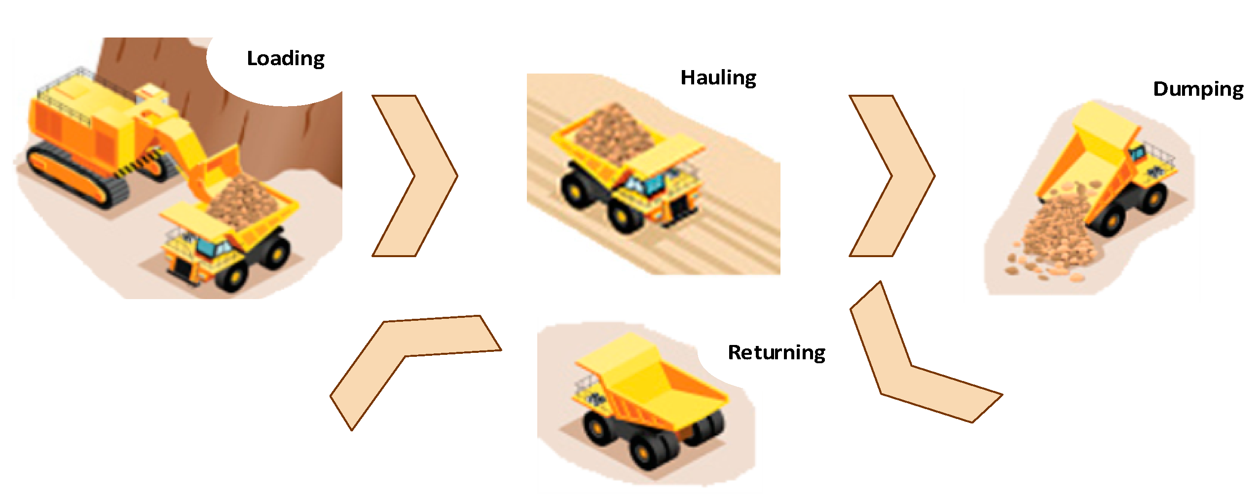
Earthmoving consists of several tasks, as shown in Figure 1, some of which include excavating, loading, hauling, dumping, crushing, and compacting [2]. The excavator/loader loads the hauler (i.e., truck) with the disposal material, the hauler starts its trip to the dumping zone, then the hauler dumps the material. Finally, it returns to the loading zone to begin the cycle anew. Earthmoving operations depend on heavy equipment for their various tasks, all of which require planning and control of the relevant methods and resources involved [3].
In a land-based operation, the main goal is to implement the project with a minimum operating cost. A critical factor to this implementation is the role of machinery and their efficient selection and management in order to minimize the overall operation costs. Due to the large scale of heavy construction projects, even a small improvement in operational efficiency could be highly cost-effective [4]. Making the right decision for an earthmoving project on both a strategic and tactical level is considered one of the most challenging phases of the project [1]. Decisions on a strategic level, i.e., long-term decisions, include both the type of equipment to be purchased or leased, and the equipment quantity. These decisions can determine if the project can be executed while complying with time and cost constraints [1]. Decisions on the tactical level, i.e., short-term decisions, include management of equipment operations, and solving unexpected issues that arise due to the uncertainty of operation processes [1]. Many difficulties can be encountered due to the nature of construction operations. These difficulties include: (1) the complicated interaction between the different resources needed to execute the required task, (2) the uncertainties and varying conditions that occur during execution that can affect operations, and (3) variability and the dynamic nature of the construction industry [5]. The recommended technique to overcome the abovementioned difficulties is the employment of computer simulations in order to model and predict the uncertainties encountered in construction operations [6]. Computer simulation can aid in the decision-making process, resulting in cost savings and increased productivity [7]. This research aims to provide a stochastic based decision-support tool for earthmoving operations to achieve the best equipment arrangement based on specific project objectives and equipment specifications utilizing empirical data. The activities’ sequence and duration are captured through simulation modeling and distribution fitting. The Decision-Support Model provides a range for optimal fleet arrangement by considering different number and types of loading and hauling equipment. The Estimating Model provides cost implications and interactions between cost, duration, and risk. The simulation is based on empirical data from construction projects, subjected to different project parameters such as: the day or night shifts, loaded dirt, and fuel consumption. Statistical distributions are used to capture activity uncertainties. The proposed decision support system consists of two parts, the Decision-Support Model, and the Estimation Model. The Decision-Support Model provides an initial prediction of the number of required trucks based on the highest possible utilization of loaders and trucks. The initial value of truck numbers is then used in the Estimation Model to estimate the cost and project duration and to perform trials around this initial estimation to achieve a project-cost tradeoff. Herein, a case study is presented in the results section to validate the developed framework of this study.
In common practice, the equipment required for a project is selected using average operating cycles, neglecting the stochastic nature of operations and equipment. Ultimately this can lead to rough estimates and poor results in meeting the projects’ objectives. The overarching research question in this article is “How to optimize earthmoving fleet arrangement by relying on empirical earthmoving data and considering interacting and influencing parameters?”.
Particularly, this research attempts to answer the following questions:
- (1)
- How to select proper fleet size and arrangement while considering the uncertain nature construction operations?
- (2)
- How to balance project cost, schedule, and level of risk/uncertainty when comparing different equipment types and fleet arrangement?
- (3)
- How project cost and duration interact considering the uncertainties involved in the day to day operations?
Specifically, this study strives to address the following objectives:
- Developing a Decision-Support Model for optimizing earth moving fleet arrangement.
- Developing an Estimation Model in the Symphony.net modeling environment to incorporate the cost aspect in the overarching model.
- Creating simulation models utilizing the empirical distributions from the previous step.
- Implement the decision support model with the goal of maximum utilization of a loader, as the loader is the most expensive resource in this study.
The potential stakeholders of the scope of this study are local agencies, planners, superintendent, project manager, equpiement owner, contractor, sub contractor, client, and logistics sectors. By employing the developed simulation model of this study, they would be able to optimize earthmoving fleet arrangement time and cost more efficiently. The simulation model enables them to plan for uncertainties and measure the cost implications of different fleet arrangements.
2. Literature Review
2.1. Modeling and Simulation
Earthmoving operations encompass a sizable portion of infrastructure projects. Mining and heavy construction projects, such as highway and dam construction, require different equipment and methods of construction. Therefore, the optimal use of resources is a critical task for contractors. Optimizing earthmoving operations has involved the development of various models employing different techniques, including simulation optimization [6,8,9], simulation and genetic algorithm (Parente and Gomez) in [10], computer simulation [11,12], linear programming [13], and artificial intelligence [14].
Simulation is defined as “imitation of a real-world process or system over time” [15]. Computer simulation tools are used to build models to provide an image of different project activities, resources used in work execution, and the surrounding environment of the project [16]. Models can be used in developing better plans for projects, optimizing the usage of resources, minimizing project costs and duration, and improving overall performance and productivity [16].
Construction simulation is the application of computer-based systems to model construction operations to understand their behavioral pattern and make decision-making models more precise [17]. When construction projects are longer and more complex, they become more challenging to manage with traditional methods; computer simulation methods can be useful in analyzing such problems. The diversified evolution of the construction simulation tool has expanded, along with the scope of its application. Various scenarios can therefore be tested to overcome real-life construction project problems. Typically, the main goal in such simulations is to minimize costs and project duration, and to explore various operation scenarios in different project types. Simulation tools can provide a holistic image of the long-term and cyclic operations which serve to generate more reliable results for these operations as compared to other methods [16]. The simulation models are built through four consecutive phases: (1) determining the product to be built, (2) abstracting and reducing the resources, processes, and environment to models, (3) carrying out the simulation and testing the model, and finally, (4) the decision-making phase [16].
2.2. Simulation in Construction
Computer simulation has also been used in other aspects of the construction process such as scheduling and planning. Liu et al. [18] established an integrated scheduling platform under resource constraints, and Bi et al. [19] conducted a schedule risk analysis to study long-distance diversion tunnels. Moreover, Lin et al. [20] employed multi-objective optimizations for construction resource allocation schemes. Tang et al. [21] investigated the impact of construction management strategies on project greenhouse gas emissions using interactive simulation. Additionally, Alzraiee et al. [22] developed the dynamic planning of construction activities by employing a hybrid simulation model to study both the operational and strategic planning aspects of a project. Finally, [23] utilized real-time data to develop a framework to simulate earthmoving projects using location tracking technologies.
Discrete event simulation (DES), a stochastic modeling method that incorporates random variables and follows a specific probability distribution, has been employed to model cyclic operations and to analyze complicated construction systems [24,25]. Several construction simulation systems have been developed within the last fifty years. For example, CYClic Operation NEtwork (CYCLONE) which was first introduced by [26], works by making modifications to the conventional Activity Cycle Diagram (ACD) to give a clearer image of different activities that are carried out in construction operations. MicroCYCLONE, which is a site level construction processes simulation program, was developed by [27]. Later, CYCLONE was further advanced as a graphical simulation software through the introduction of State- and ResOurce-Based Simulation of Construction ProcEsses (STROBOSCOPE) [28] and EZSTROBE [29]. SIMPHONY was developed in 1996 and was considered one of the most successful simulation software that aids the modeler in developing complicated models by using a user-friendly interface [30]. Simplified Discrete-Event Simulation Approach (SDESA) was first introduced in 2003, leading to the development of the ACD simulation method and the proposal of the disposal resource concept [31]. A further development was introduced in the construction process simulation by developing the Simphony.NET 3.5 [17] and COSYE [30] based on the concept of High-Level Architecture. Ince [6] developed a simulation model that dynamically predicts the Roughness Defect Score of the road as the traffic increases and gives an optimal maintenance management program based on the impacted cost parameters by employing Simphony.Net. Additionally, Ince incorporated a Markov model in the system to accommodate a more realistic modeling of the road deterioration status over time.
There are primarily two components involved in construction simulation models, activity, and resource [16]. These refer to the activities involved in a project, and the resources required to accomplish those activities. Construction activities have a degree of uncertainty, due to the stochastic nature of their processes, and several parameters that affect productivity and performance. Labor skills, weather conditions, and equipment breakdown are just a few examples of the uncertainties involved during the duration of construction activity [32]. Modeling all possible factors of influence would be a daunting task. Even if every aspect of an operation is modeled, it would be near impossible to properly include all site conditions and factors that can occur while executing the project. Comparably, it would be too simplistic to rely on average cycle times and choose an integer value for the number of equipment without considering the consequences. An appropriate solution then, is to simulate the operation activities stochastically. As a result, the simulation would not have constant activity durations; activity durations would be randomly selected from its associated probability density, representing the reality on the ground [17]. Moreover, the success of a simulation experiment depends mainly on the accuracy of the input modeling [1]. In developing a simulation model for construction processes, the models can be based either on observations of historical data, or an experts’ judgment and knowledge of the processes [33]. The use of historical data is advisable when the user does not expect any significant change in the underlying assumptions of the process. While the experts’ judgment is an appropriate choice for conceptualizing inputs that are expected to vary in the future due to unexpected changes in the underlying factors.
After reviewing the role of simulation in the construction industry, and the modeling of stochastic durations, it is essential to discuss the reasons behind modeling earthmoving operations. According to [34], an earthmoving simulation model should address the following: (1) modeling earthmoving operations in a simple way to understand and providing a clear image of the process, (2) modeling complex construction operations and increasing the productivity of operations, (3) visualizing the complex and dynamic interactions between different activities and resources, (4) optimizing the earthmoving operations in terms of fuel consumption, productivity, and resource utilization, and (5) reducing the fuel consumption for haulers (trucks) for both monetary and environmental reasons.
2.3. Identified Gap
The focus of this study is in optimizing earthmoving operations. Earthmoving operations are costly and involve many different variables that once optimized can lead to significant savings of cost and time. In earthmoving operations, you deal with four main activities including loading, hauling, dumping, and returning. These activity durations are impacted by uncertainties resulting in a stochastic behavior [34]. Earthmoving operations have many interacting activities and resources that need to be planned accurately to ensure successful project execution. As a result, a comprehensive and adaptable modeling approach is needed to address this complexity. There have been multiple studies carried out in the past three decades for modeling the uncertainties in a earthmoving operation that indicate the uniform, triangular, normal and lognormal [35], beta [33], and Erlang [36] distributions are suitable for expressing the uncertainties in construction processes. AbouRizk and Halpin [33] recommended using flexible distributions with tractable parameters that can be estimated from sample data and should be bounded between upper and lower limits. This approach was adopted in this study to model the uncertainties in the production and consumption rates of the heavy machinery.
3. Methodology
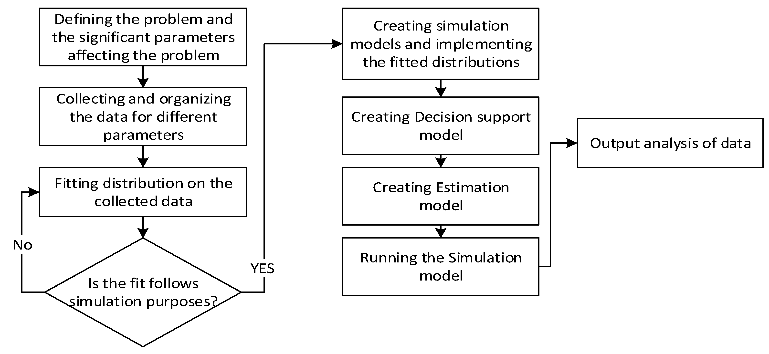
This research aims to provide a decision support tool through a simulation model that is capable of modeling earthmoving operations in terms of the total cost of ownership (TCO), fuel consumption, productivity, and resource utilization. Figure 2 illustrates a flowchart of the methodology presented in this research. A problem or gap in the industry is defined along with and the leading parameters affecting the earthmoving operation (In common practice, the equipment required for a project is selected using average operating cycles, neglecting the stochastic nature of operations and equipment. Ultimately this can lead to rough estimates and poor results in meeting the projects’ objectives.). Empirical data for different parameters under the study is collected and organized, and various distributions on the collected data is fitted to find the representative distributions for each parameter. Particularly, this study strives to address the following objectives:
- Developing a Decision-Support Model for optimizing earth moving fleet arrangement.
- Developing an Estimation Model in the Symphony.net modeling environment to incorporate the cost aspect in the overarching model.
- Creating simulation models utilizing the empirical distributions from the previous step.
- Implement the decision support model with the goal of maximum utilization of a loader, as the loader is the most expensive resource in this study.
Ultimately, these objectives resulted in a prediction model covering the cost estimation aspects of the earth moving project that is based on realistic assumptions.
A basic earthmoving project can be summarized into four significant components: the loading, hauling, dumping, and returning of trucks. However, selecting the proper number of trucks considering the cost and duration of the project, while maintaining allowable confidence levels may not be a straightforward task. Figure 3 depicts the activities and steps that each truck follows to assist in the completion of an earthmoving project. This abstraction is adopted for simulation purposes in this study. All durations of the activities illustrated in the following flowchart, as well as the amount of dirt being moved by each truck, have a stochastic nature, and follow a probability distribution in the real world. The problem defined in this research is how to select the proper fleet size and configuration given the uncertainties in the nature of an earthmoving fleet’s activities and operations. Parameters such as truck types and capacity, loader bucket capacity, hauling speed, and many more (listed in Table 1) can have a major impact on fleet selection, as well as the cost and duration associated.
The cost components that affect an earthmoving project can be defined as the operational cost of equipment (i.e., the hourly equipment cost for owner and operator costs), and the fuel cost. In reality, these values are not constant and depend on the idle time of the truck and hauling distances. Capturing and including this variation in a simulation model is one of the advantages to this research. The list of all the simulation variables used in this study is illustrated in Table 1.
4. Case Study
The duration and productivity of construction activities can experience uncertainties best captured by a range of distributions. The range of each activity is governed by the parameters affecting that activity, and to some extent can be obtained by analyzing activity duration/productivity over time. As a result, the more data gathered, the more accurately parameters and ranges can be generalized to fit a problem. To give a full scope of the earthmoving variables and parameters, the data encompassed in this study is provided for two truck types and two loader types under the same soil conditions. The data set collected in this research includes more than 1400 data points capturing the duration of all the activities in heavy haul operations with 750 data points from the day shifts and 650 data points from the night shifts. As a result, two 10-h shifts were taken on every 24-h day. To make the simulation results more generalizable to possible scenarios, distributions were fitted to the collected data with the defined parameters in Table 1, considering the following two concepts:
- Distributions should be at bounded on the left side as the duration or fuel consumption cannot have negative values.
- For simulation purposes, having the right side unbounded could result in irrationally large numbers, which may cause an error in the simulation.
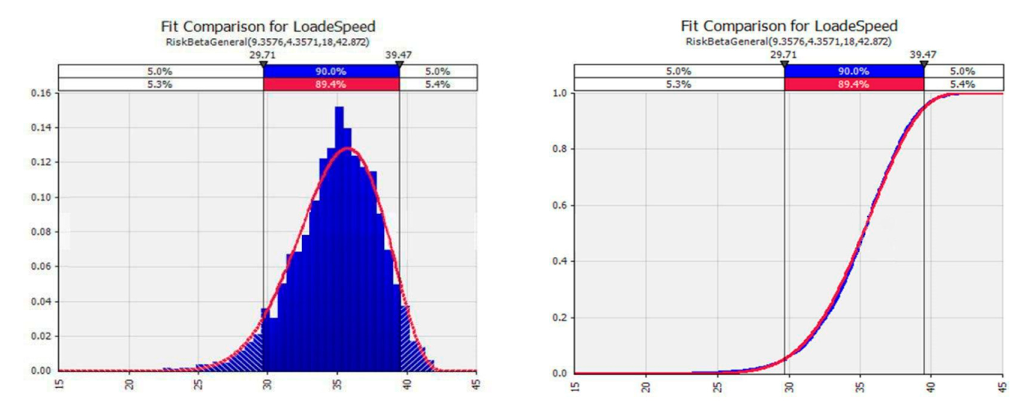
Based on the abovementioned assumptions, the most reliable distributions for the parameters defined in Table 1 were limited to three distributions of Beta, Triangular, and Uniform. Table 2 represents the best fitted distribution to each uncertain parameter. Figure 4 also depicts a sample distribution fitted to the loading rate of the loader activity. The following shows the description of the activities:
- Excavator Loading rate (CY/minute): Refers to the capacity (cubic yard) of each rotor bucket in cubic yard, per minute.
- Truck Loaded Speed (Mile/hour): Refers to the speed (Mile/hour) of the loaded truck.
- Truck Payload (CY): Refers to all the cargo weight that you can safely add in addition to your truck’s empty weight.
- Truck Dumping time (Minute): Refers to the time (Minute) required to dump the material.
- Excavator Fuel consumption Rate (Gal/hour): Refers to the fuel consumption volume (Gallon) of the excavator in each hour.
- Truck Cycle Fuel (Gal/Mile): Refers to the fuel consumption volume (Gallon) of truck by completing each earthmoving cycle.
4.1. Creating Simulation Models Utilizing the Fitted Distributions
From a decision-makers’ point of view, allocating the right amount of resources for each activity can play a crucial role in determining the project cost and duration.
The factors contributing to these can change from one project to another, depending on the choice of equipment, hauling distance, and number of resources. This problem is addressed in the next two sections; first, a simulation model with the purpose of identifying the range of optimal fleet size is developed; second, a model with more detailed cost functions captures the true operation costs and can perform a more detailed comparison of the range of fleet sizes provided by the Decision-Support Model.
4.1.1. Decision-Support Model
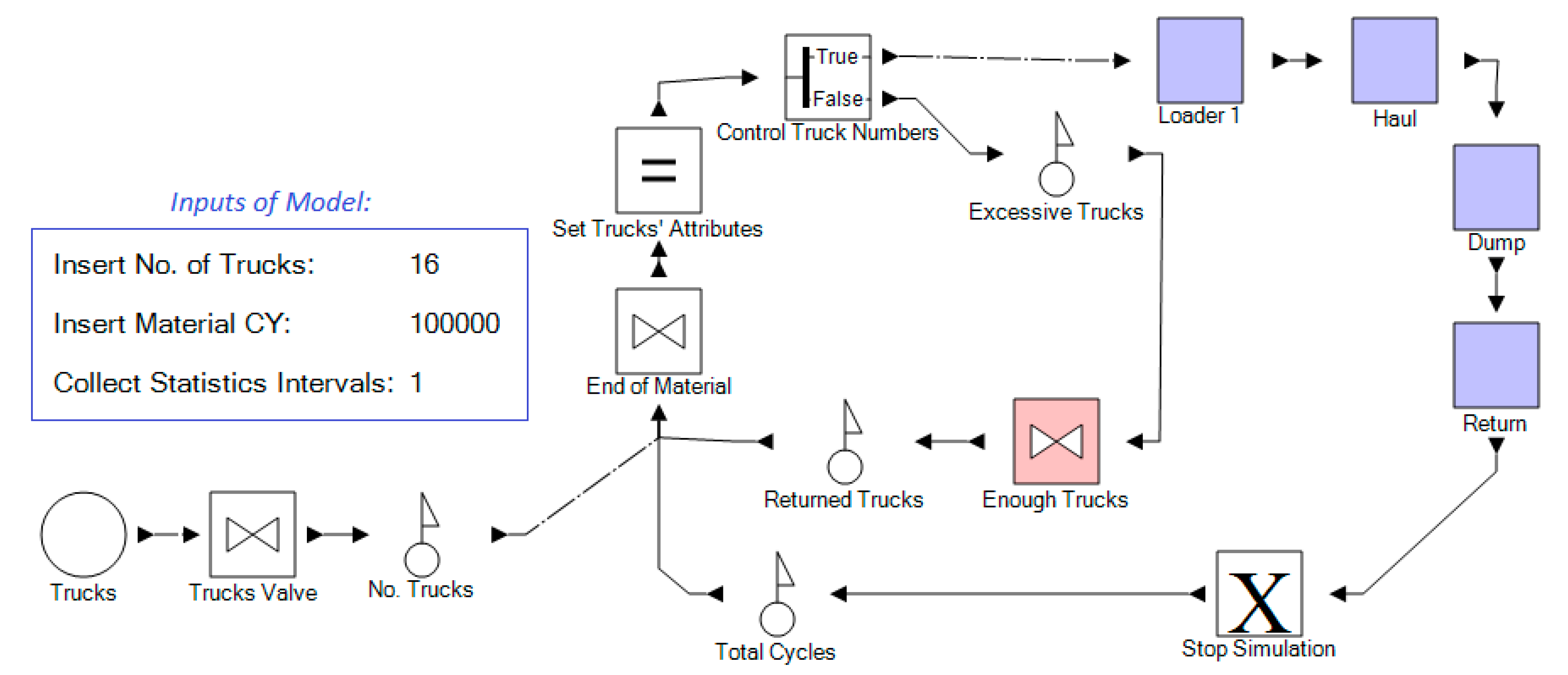
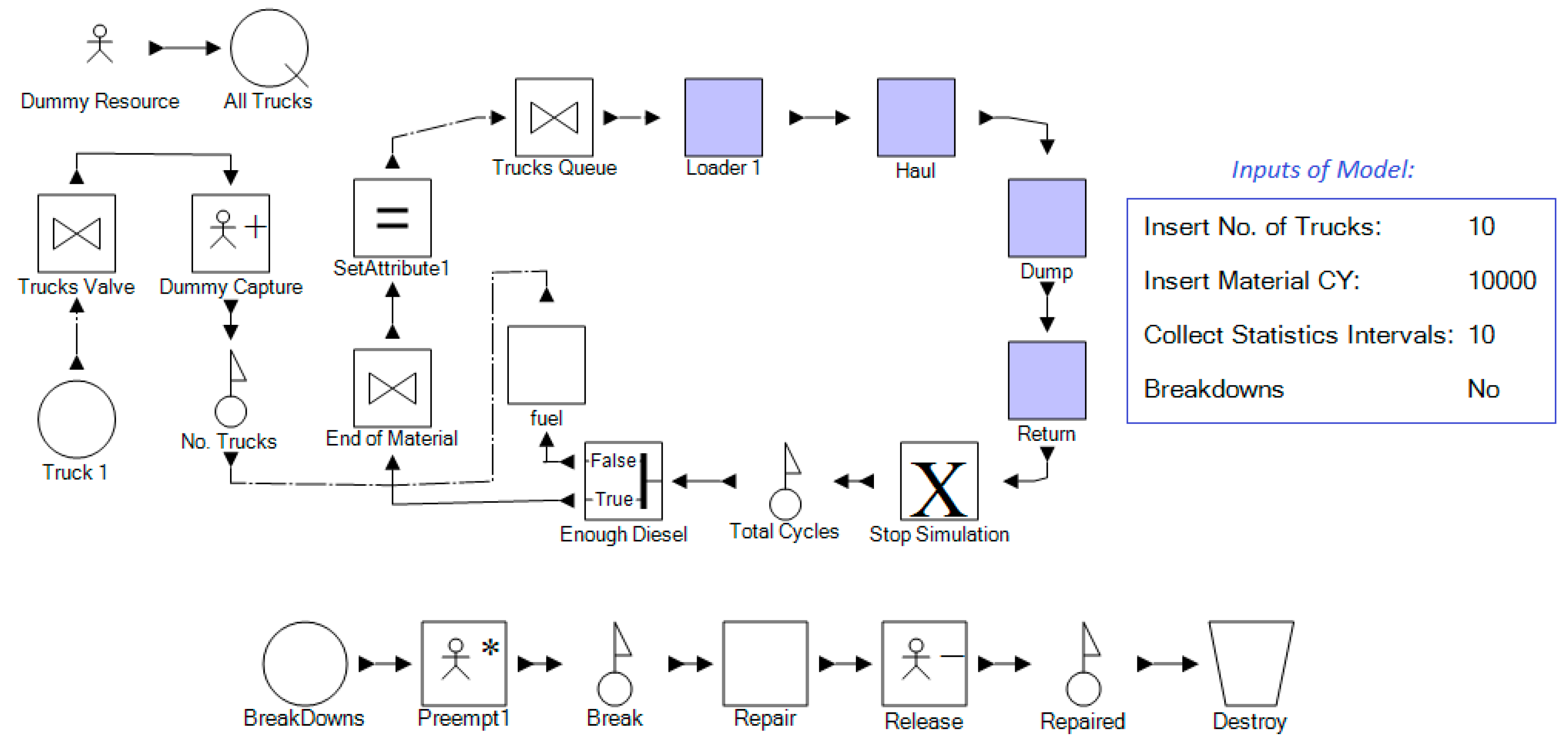
The Decision-Support Model has all the attributes of the hauling operation but has more freedom in changing its fleet size during operations. The model is structured with a main loop performing the primary operation activities and a secondary loop of capturing excessive trucks or releasing more as needed (Figure 5). The main loop consists of all activities in the hauling operation, with the activity durations randomly sampled from the distributions discussed in the previous section. The second loop, shown in Figure 5, incorporates values and conditions for the capturing and releasing of trucks. This method results in the full utilization of the loader as the most expensive resource. Moreover, this method can illustrate a range of fleet sizes as opposed to one value, due to stochastic nature of these operations. This model sampled the loading, hauling, dumping, and returning durations of trucks along with the trucks’ loaded dirt from the distribution as defined in the previous step. The element of “Set Trucks’ Attributes” assigned trucks properties (e.g., hauling duration) to flow entities (i.e., trucks). Every truck carried a certain amount of dirt, so when there was no material to be hauled, trucks stopped in the “End of Material” element. The simulation was terminated by having the specified material hauled.
In parallel to the cycle depicted in Figure 5, a separate cycle, highlighted in Figure 6, collected statistical information from the primary cycle during every identified collection interval. As a result, as the simulation progressed, the data (such as the number of trucks in every instance of the simulation) was collected for statistical analysis.
4.1.2. Cost Estimation Model
After comparing the initial output of the first simulation over system performance, a more comprehensive model was developed covering the cost estimation aspects of the project with a more detailed consideration to cost. Figure 7 illustrates the Cost Estimation Model developed in this study. In said model, some elements were defined with exact properties and functions identical to the Decision-Support Model, while new functions were elaborated as follows:
- A dummy resource was captured as each truck was being generated to mimic truck breakdowns in every instance of the simulation.
- Preempting this dummy resource halted trucks within tasks and released it after it was repaired, returning the truck to its task.
- Fuel consumption of trucks was defined as: idle fuel consumption + moving or cycle fuel consumption.
- The duration that each truck was idle (fuel consumption) before getting loaded by the loader was measured in the “Trucks Queue” element (when multiplied by idle fuel consumption rate results in idle fuel consumption).
- Cycle fuel consumption was calculated by checking the state of diesel in the truck fuel tank before and after each cycle.
- If the level fuel in a truck’s tank after each cycle was less than that required for the next cycle (with a margin of 20 percent), the trucks needed to fill their tanks. This condition was modeled in the simulation by the “Enough Fuel” element.
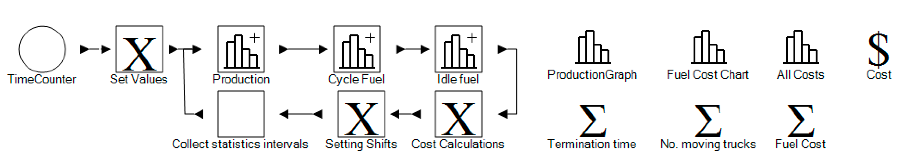
The statistical information of the simulation was collected by a parallel cycle which also simultaneously set shifts and calculated costs Figure 8 depicts the statistical information collection process of the estimation model developed in this study. Additionally, the intervals between data collections were set implicitly by inputting a task inside this cycle.
Table 3 shows the assumptions of this study for the price of loaders and trucks, the capacity of the trucks’ tanks, and the diesel price. These assumptions were implied to be deterministic due to their nature, as the user would know the exact price and capacity tank at any given time.
The estimation model simulation started with a sampling from the distributions on created process models and by running a Monte Carlo simulation (with 1000 runs). The decision-making model output is the number of trucks that results in the maximum utilization of the loader. Whereas, in the estimation model, more comprehensive details about the costs related to the project are considered. The results of the simulations are presented and discussed in the next section.
5. Analysis of the Results and Discussion
The output analysis of this simulation ultimately could facilitate the decision-making process in earthmoving projects, taking into considering cost and duration. As long as the assumptions within the models (e.g., cost of fuel) are consistent, the outcome is comparable between different arrangements of truck and loaders. Many aspects of an earthmoving project can be analyzed by performing this simulation for the defined scenarios, resulting in better overall project decisions made with increased confidence.
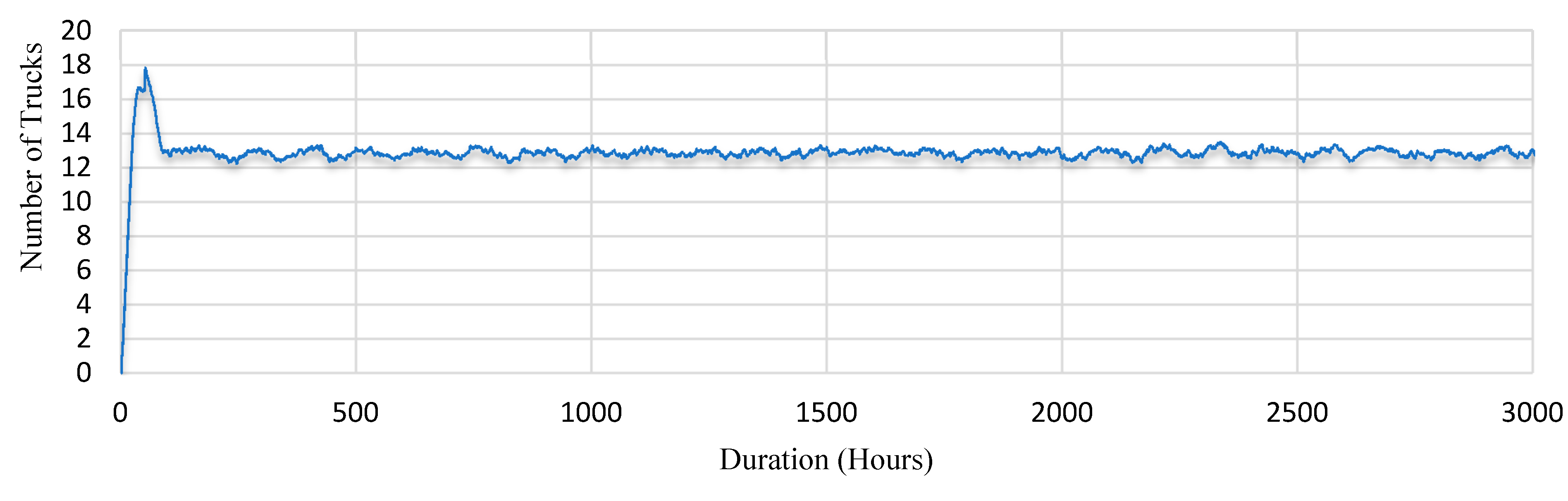
From the decision-making model, the number of trucks that results in the highest utilization of the loader can be obtained. Assuming a fixed hauling distance (40 miles in this case), the project production rate is controlled by the loader reaching one hundred percent utilization rate. Figure 9 depicts the optimum number of trucks needed to achieve one hundred percent utilization of the loader during the simulation period. At the beginning of the simulation, the model releases more trucks, as requested by the loader. It is noteworthy that the peak at the beginning of the simulation appears because the first loaded trucks have not yet returned from the dumpsite. In other words, whenever the loader is idle another truck is requested. After the initial phase, the feedback loop stabilizes the system and reduces the number of trucks. Due to the uncertain nature of operation, there are still fluctuations in number of trucks, but the fluctuations are in between 12–14 trucks. As time passes, the number of trucks required fluctuates between twelve and fourteen. These fluctuations are capturing the operations’ uncertainty and stochastic nature.
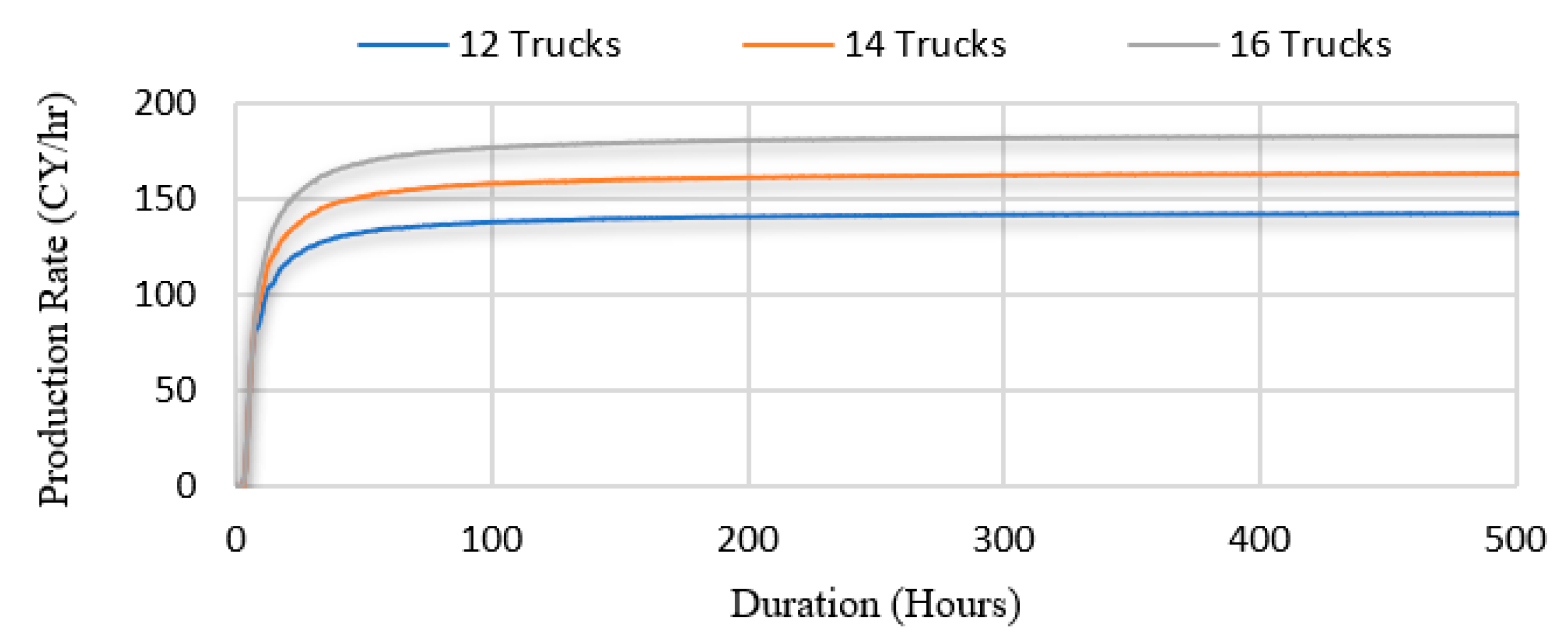
The loader–truck configuration can be further investigated in the Cost Estimation Model using the information gathered from the Decision-Support Model. The first value that could be useful to a project manager is the production rate, calculated based on the slope of production over time. Figure 10 shows the production rate for different numbers of trucks in units of a cubic yard per hour. As a result of the stochastic nature of the operations, adding more trucks increases loader utilization (Figure 11) and therefore improves the production rate (Figure 10), at a cost. Figure 11 compares the average number of trucks waiting in the loader’s queue and their average waiting time for different truck–loader configurations.
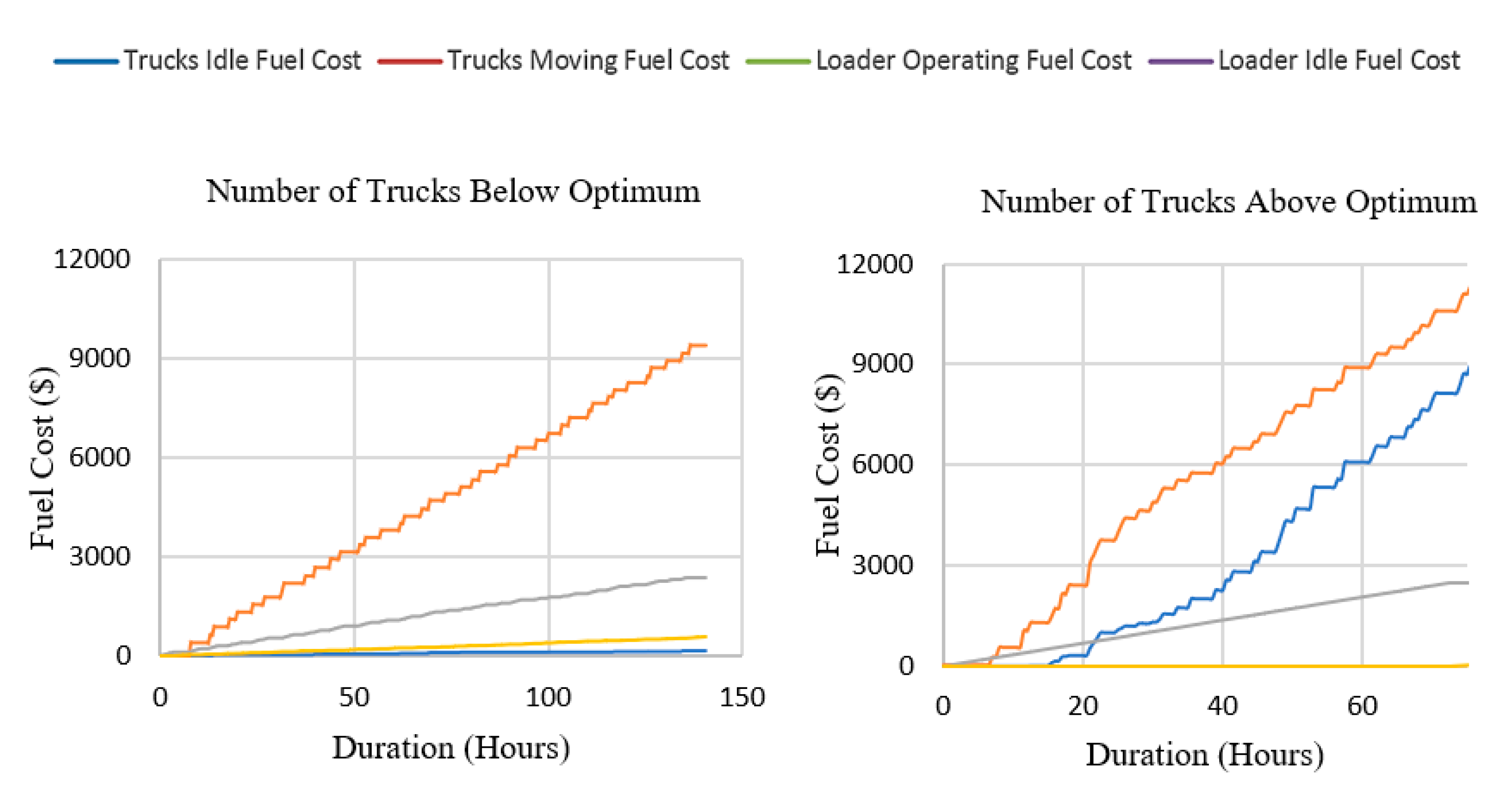
To demonstrate the functionalities of the Cost Estimation Model, we can investigate the fuel consumption over time for scenarios with a number of trucks above or below optimum values. Figure 12 shows the fuel cost of the project for a short period. In the case where the number of trucks is less than the optimum (12 trucks), the idle fuel cost of the loader increases, while the truck’s idle fuel cost is significantly reduced. On the other hand, when the number of trucks is higher than the optimum (18 trucks), the idle fuel cost of the loader is reduced, and the truck’s idle fuel cost increases (Figure 12).
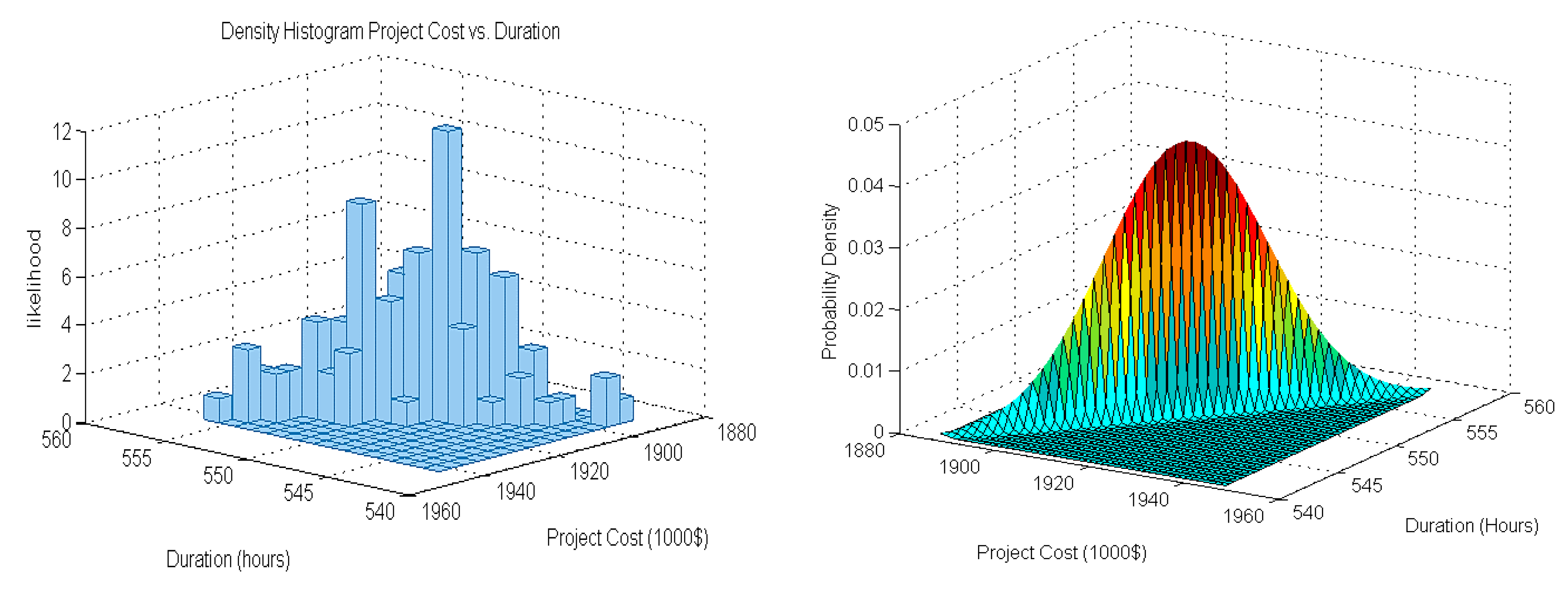
One of the most significant requirements of such a simulation is to generate results incorporating the stochastic and uncertain attributes of the model. In terms of an earthmoving project, project duration and cost, and more importantly their interaction, plays a critical role in project planning and success. The output of a stochastic model would be a non-crisp value, which can form a bivariable histogram of cost–duration. If the collected output data is well distributed over the given range of outputs, it can form a normal distribution. The bivariate cost–duration distributions’ results of this study are shown in Figure 13. The histogram and distribution demonstrate a superior fitting accuracy and generalization. A clear correlation between the cost and duration is also visible.
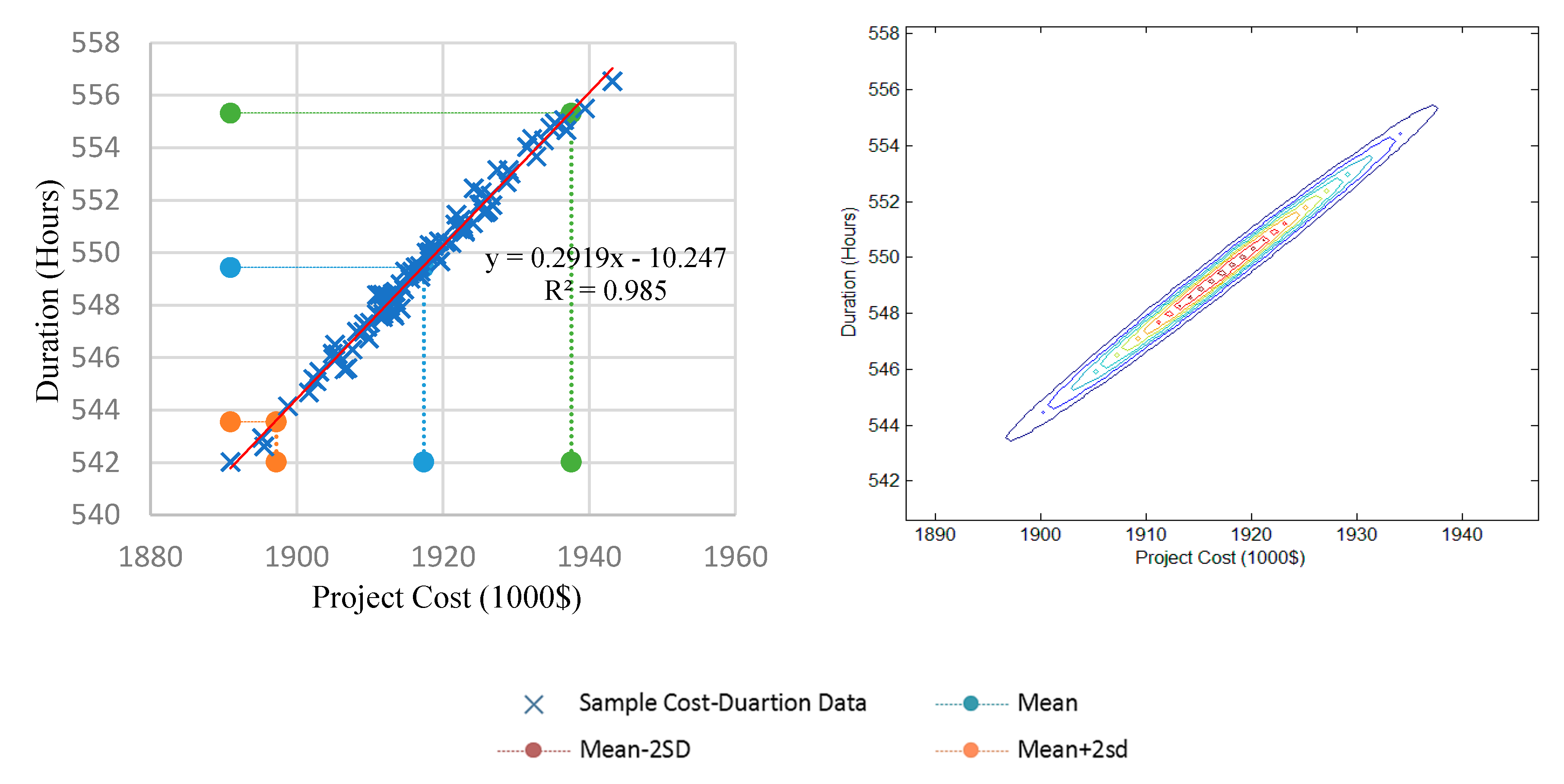
Figure 14 shows a sample of the scattered cost and duration results for a specific truck and loader arrangement. For each arrangement of trucks and loaders, a positive correlation and dependency can be observed between project duration and cost.
The results of the simulation for different arrangements of trucks and loaders makes it possible to compare different scenarios and perform value engineering for a specific project. Figure 15 depicts project duration and cost samples for truck type 1 and loader type 1 arrangements. Three key observations can be derived from Figure 15; first, the increase in project duration is much more significant when changing the number of trucks from 14 to 12, compared to the change of 20 to 18. Second, the result of simulation models indicates that the greater the number of trucks the steeper the ratio between cost and duration. Third, the spread (standard deviation) of the simulation results between different truck numbers shows the uncertainty of each scenario. The cost–duration results of a 12-truck case shows a much higher variance than a 15-truck case.
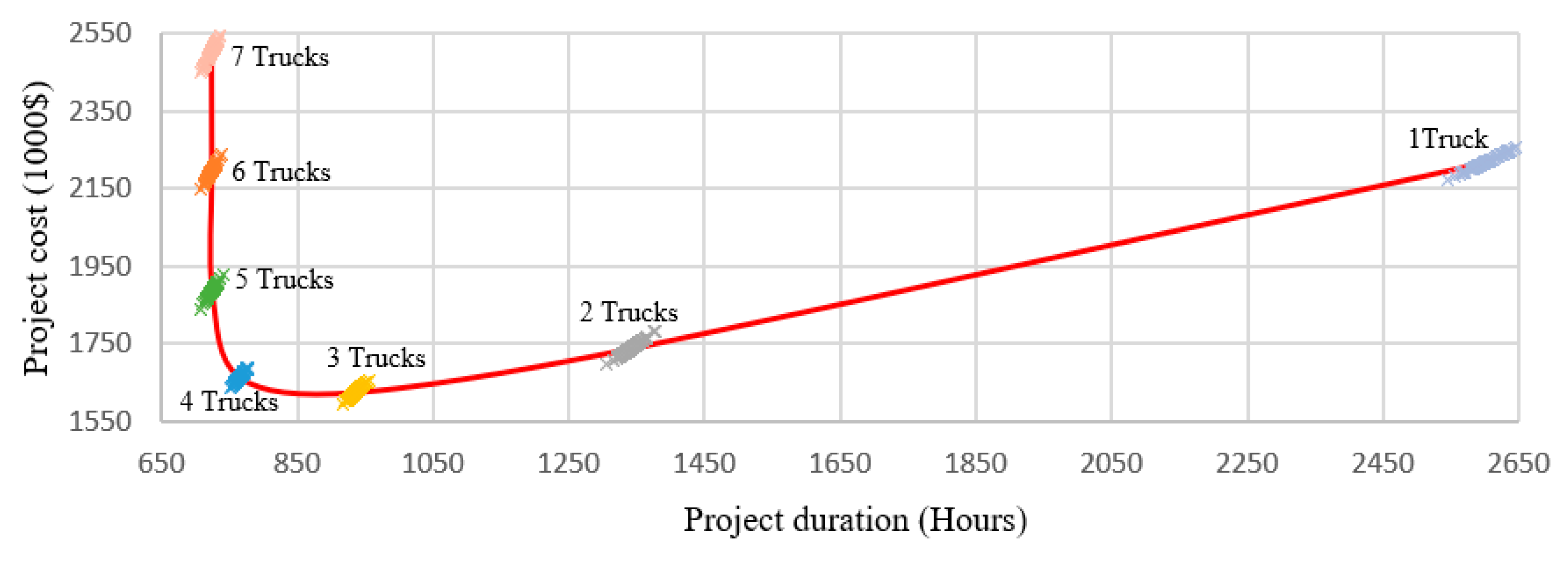
Figure 16 shows a separate equipment arrangement (for truck type 2 and loader type 2 arrangements) simulation result. The high cost of loader underutilizing has been added to the project costs, compared to the scenario with truck type 1 and loader type 1 arrangements (Figure 15). This is increasingly evident in the truck 1 results at the right end of the figure. Another noticeable difference between the results in Figure 15 and Figure 16 is that the steepness of ratio between cost and duration is much higher in the type 2 arrangements. More specifically, by changing the number of trucks from 7 to 6 or 5, the duration does not change significantly, but the total cost drops considerably. However, by changing the number of trucks from 4 to 2 and from 2 to 1, the cost and duration of the project significantly increases, and the increase in the duration is greater than that in cost.
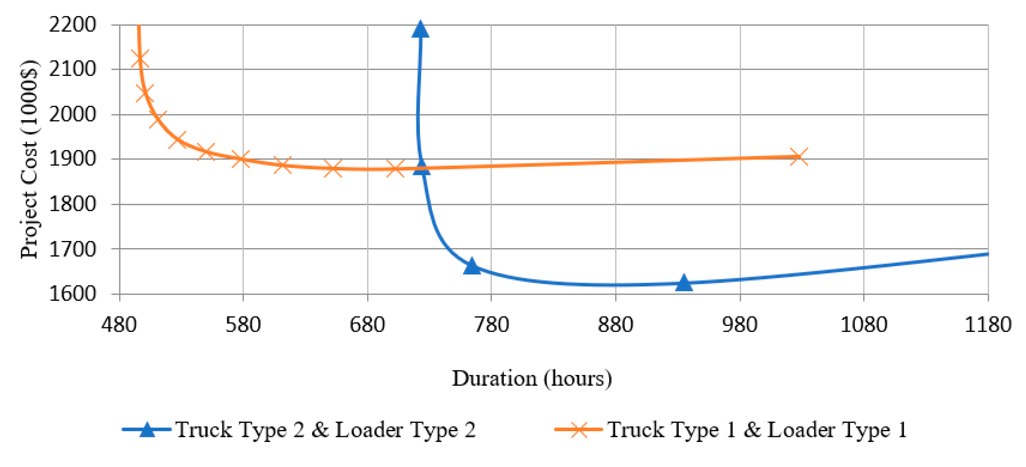
The mean curve of the projected cost and duration of the project for both fleet arrangements (Figure 15 and Figure 16) are plotted in Figure 17. In the planning stages of a project, such graphs can be generated to improve project visibility and predictions. Furthermore, comparing different fleet configurations and arrangements can benefit the user and facilitate optimal decision making regarding the preferred time and cost of the project.
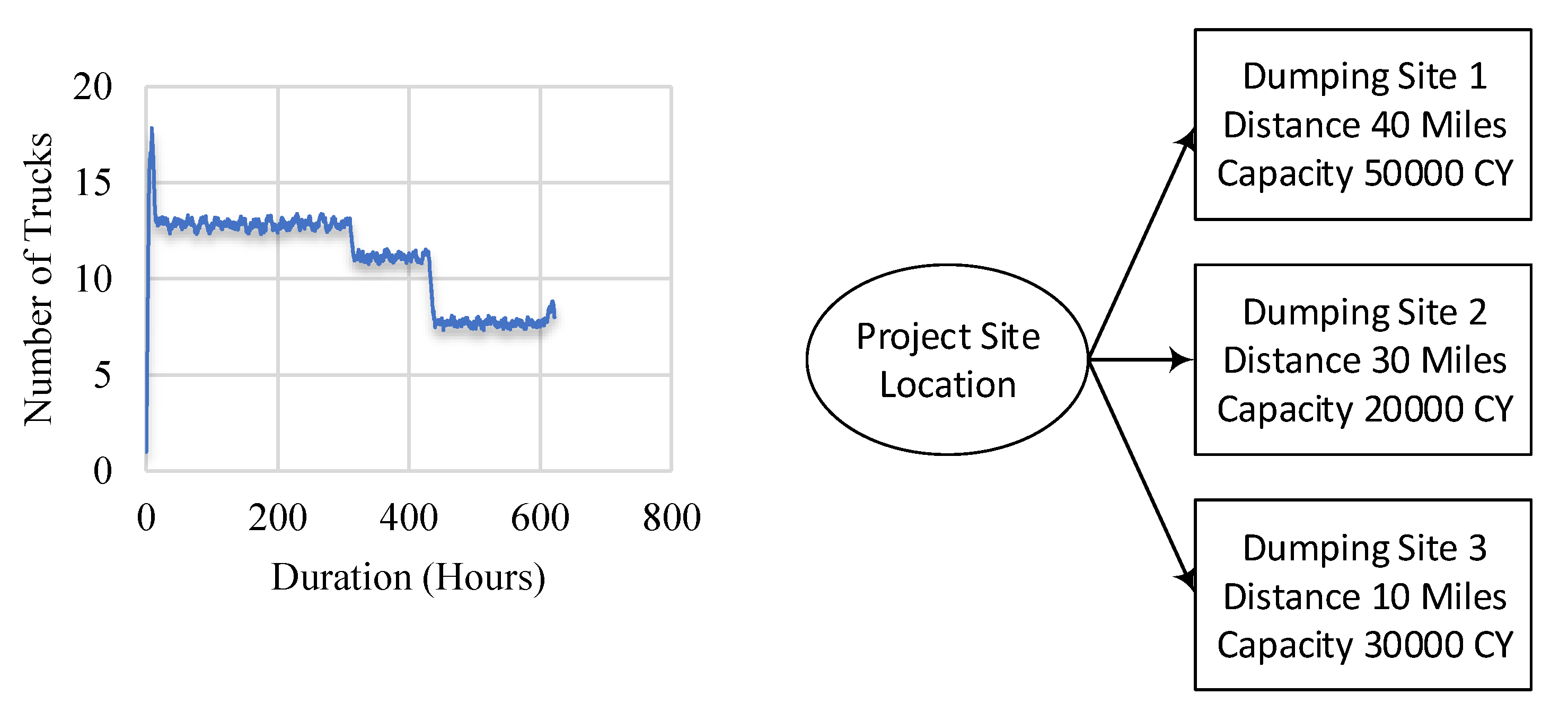
In all the previous sections, the hauling distance is assumed to be constant (40 miles), wherein most of the cases there is more than one dumping site. The simulation model presented in this study can quickly adapt to the changing environment by finding the optimum fleet management for such cases and further comparing the cost of a change in resources, i.e., changing the number of trucks throughout the project or keeping set resources for the duration. Figure 18 demonstrates that by using the same framework presented in the Cost Decision Support model, only changing the hauling distances, the proper number of equipment can be obtained.
6. Conclusions
Operation simulation is identified as an efficient technique to model and analyze the stochastic aspects of the cost and duration of earthmoving operations in construction projects. Therefore, two simulation models—namely the Decision-Support Model and the Estimation Model—have been developed in the Symphony.net modeling environment to address the industry needs in optimizing fleet arrangement. The Decision-Support Model provides the best arrangement of equipment to maximize global resource utilization. In contrast, the Estimation Model captures more of the project details and provides a comparison of various equipment arrangements based on their cost. This research adds to the construction equipment management body of knowledge by providing a framework for developing stochastic simulation based on empirical data to capture cost–benefit ratio (CBR) of deferent fleet arrangements considering the correlation between cost and duration for different scenarios. The findings of this study can be summarized in three main areas:
- Cost–benefit ratio (CBR) of an increase or decrease in fleet size, i.e., the relationship between cost and fleet size is not linear (evident in Figure 15).
- The correlation between cost and duration for different scenarios needs to be understood to make sound decisions on fleet management.
- Stochastic simulation based on empirical data is an appropriate tool for assessing and measuring the uncertainty and risk of fleet scenarios.
The absence of a customized simulation model to incorporate and synchronize the fleet resources for earthmoving projects results in projects that are prone to cost and time overruns. A proper simulation could provide great insight in dealing with sophisticated fleet selection and multiple routing scenarios. Other planners, engineers, and scholars can follow the proposed process in this study to generate the charts and optimize the cost–time management considering the uncertainty and characteristics of their construction projects. Performing simulation analysis in the planning stages of the project can lead to significant cost savings in project execution and provide excellent visibility of project performance. The graphs developed in the process of the simulation can become quick decision support guidelines for future projects and ad hoc decisions. The proposed tool provides a practical project management approach, yielding notable cost, time, and resource savings during the planning and execution phases of construction projects. In this paper, these models are developed, and the modeling logic is validated through a case study employing a real-world earthmoving project in Canada that demonstrates the model’s capabilities. This demonstration demonstrated the model’s usefulness, presented its crucial features, and facilitated its assessment.
The main limitations of this research include data magnitude (The data set collected in this research includes about 1400 data points capturing the duration of all the activities in heavy haul operations with 750 data points from the day shifts and 650 data points from the night shifts); to increase the accuracy of the prediction of the simulation model, more data is required. There are more complex modeling approaches such as machine learning and deep learning which were not included in the pipeline.
For future studies, researchers can examine various arrangements of the number of resources and add other types of heavy-duty machines to analyze the construction process more comprehensively. Moreover, they could also add several economic and construction independent variables to investigate how these factors affect earthmoving projects. Additionally, linear, and non-linear regression models can be utilized to study the arrangement of heavy-duty vehicles in construction projects, and their impact on time and cost attributes. Furthermore, additional project risk factors such as equipment breakdown, weather conditions, and labor skill set can be incorporated into the models for achieving more reliable fleet arrangement. Additionally, scholars could enhance the generated model more accurately by adding the maintenance cost of each cycle. Ultimately, it is crucial to study the effect of the contractors’ management style on earthmoving fleet arrangement.
Author Contributions
Conceptualization, A.M. (Arash Mohsenijam) and A.M. (Amirsaman Mahdavian); methodology, A.M. (Arash Mohsenijam), A.M. (Amirsaman Mahdavian) and A.S.; software, A.M. (Arash Mohsenijam); validation, A.M. (Arash Mohsenijam), A.M. (Amirsaman Mahdavian) and A.S.; formal analysis, A.M. (Arash Mohsenijam), A.M. (Amirsaman Mahdavian) and A.S.; investigation, A.M. (Arash Mohsenijam), A.M. (Amirsaman Mahdavian) and A.S.; resources, A.M. (Arash Mohsenijam), A.M. (Amirsaman Mahdavian) and A.S.; data curation, A.M. (Arash Mohsenijam); writing—original draft preparation, A.M. (Arash Mohsenijam); writing—review and editing, A.M. (Arash Mohsenijam), A.M. (Amirsaman Mahdavian) and A.S.; visualization, A.M. (Arash Mohsenijam), A.M. (Amirsaman Mahdavian) and A.S.; supervision, A.M. (Arash Mohsenijam), A.M. (Amirsaman Mahdavian) and A.S.; project administration, A.M. (Arash Mohsenijam), A.M. (Amirsaman Mahdavian) and A.S. All authors have read and agreed to the published version of the manuscript.
Funding
This research received no external funding.
Conflicts of Interest
The authors declare no conflict of interest.
References
- Fu, J. A Microscopic Simulation Model for Earthmoving Operations. In Proceedings of the International Conference on Sustainable Design and Construction, Zurich, Switzerland, 15–17 January 2012; pp. 218–223. [Google Scholar]
- Ricketts, J.T.; Loftin, M.K.; Merritt, F.S. Standard Handbook for Civil Engineers; McGraw-Hill Professional: New York, NY, USA, 2003. [Google Scholar]
- Edwards, D.G.; Holt, G. Construction plant and equipment management research: Thematic review. J. Eng. Des. Technol. 2009, 7, 186–206. [Google Scholar] [CrossRef]
- Asadbeigi, F.; Golsoorat Pahlaviani, A.; Majrouhi Sardroud, J. Application of Genetic Algorithms to Optimize Heavy Earthwork Operations. J. Innov. Res. Eng. Sci. 2018, 4, 94–98. [Google Scholar]
- Aytug, H.; Lawley, M.A.; McKay, K.; Mohan, S.; Uzsoy, R. Executing production schedules in the face of uncertainties: A review and some future directions. Eur. J. Oper. Res. 2005, 161, 86–110. [Google Scholar] [CrossRef]
- Ince, M. Simulation-based Modelling of the Unpaved Road Deterioration and Maintenance Program in Heavy Construction and Mining Sectors. Master’s Thesis, Lakehead University, Thunder Bay, OT, Canada, 2019. [Google Scholar]
- Klingstam, P.; Gullander, P. Overview of simulation tools for computer-aided production engineering. Comput. Ind. 1999, 38, 173–186. [Google Scholar] [CrossRef]
- Markiz, N.; Jrade, A. An expert system to optimize cost and schedule of heavy earthmoving operations for earth- and rock-filled dam projects. J. Civ. Eng. Manag. 2017, 23, 222–231. [Google Scholar] [CrossRef]
- Marzouk, M.; Moselhi, O. Object-oriented simulation model for earthmoving operations. J. Constr. Eng. Manag. 2003, 129, 173–181. [Google Scholar] [CrossRef]
- Marzouk, M.; Moselhi, O. Multi-objective optimization of earthmoving operations. J. Constr. Eng. Manag. 2004, 130, 105–113. [Google Scholar] [CrossRef]
- Kim, H.; Ham, Y.; Kim, W.; Park, S.; Kim, H. Vision-based nonintrusive context documentation for earthmoving productivity simulation. Autom. Constr. 2019, 102, 135–147. [Google Scholar] [CrossRef]
- Zhang, J.; Zhong, D.; Wu, B.; Lv, F.; Cu, B. Earth Dam Construction Simulation Considering Stochastic Rainfall Impact. Comput. Aided Civ. Infrastruct. Eng. 2018, 33, 459–480. [Google Scholar] [CrossRef]
- Son, J.; Mattila, K.; Myers, D. Determination of haul distance and direction in mass excavation. J. Constr. Eng. Manag. 2005, 131, 302–309. [Google Scholar] [CrossRef]
- Alkass, S.; Harris, F. Expert system for earthmoving equipment selection in road construction. J. Constr. Eng. Manag. 1988, 114, 426–440. [Google Scholar] [CrossRef]
- Banks, J.; Carson, J.S.; Nelson, B.L.; Nicol, D.M. Discrete-Event System Simulation; Prentice Hall, Inc.: New Jersey, NJ, USA, 2000. [Google Scholar]
- AbouRizk, S. Role of Simulation in Construction Engineering and Management. J. Constr. Eng. Manag. 2010, 136, 1140–1153. [Google Scholar] [CrossRef]
- AbouRizk, S.; Hague, S. User’s Guide for General Template in Simphony.Net 3.5; University of Alberta: Edmonton, AB, Canada, 2008. [Google Scholar]
- Liu, H.; Al-Hussein, M.; Lu, M. BIM-based integrated approach for detailed construction scheduling under resource constraints. Autom. Constr. 2015, 53, 29–43. [Google Scholar] [CrossRef]
- Bi, L.; Ren, B.; Zhong, D.; Hu, L. Real-Time Construction Schedule Analysis of Long-Distance Diversion Tunnels Based on Lithological Predictions Using a Markov Process. J. Constr. Eng. Manag. 2015, 141, 04014076. [Google Scholar] [CrossRef]
- Lin, C.T.; Hsie, M.; Hsiao, W.T.; Wu, H.T.; Cheng, T.M. Optimizing the schedule of dispatching earthmoving trucks through genetic algorithms and simulation. J. Perform. Constr. Facil. 2012, 26, 203–211. [Google Scholar] [CrossRef] [Green Version]
- Tang, P.; Cass, D.; Mukherjee, A. Investigating the effect of construction management strategies on project greenhouse gas emissions using interactive simulation. J. Clean. Prod. 2013, 54, 78–88. [Google Scholar] [CrossRef] [Green Version]
- Alzraiee, H.; Zayed, T.; Moselhi, O. Dynamic planning of construction activities using hybrid simulation. Autom. Constr. 2015, 49, 176–192. [Google Scholar] [CrossRef]
- Vahdatikhaki, F.; Hammad, A. Framework for near real-time simulation of earthmoving projects using location tracking technologies. Autom. Constr. 2014, 42, 50–67. [Google Scholar] [CrossRef]
- Bokor, O.; Florez, L.; Osborne, A.; Gledson, B.J. Overview of construction simulation approaches to model construction processes. Organ. Technol. Manag. Constr. Int. J. 2019, 11, 1853–1861. [Google Scholar] [CrossRef] [Green Version]
- Longman, M.; Miles, S.B. Using discrete event simulation to build a housing recovery simulation model for the 2015 Nepal earthquake. Int. J. Disaster Risk Reduct. 2019, 35, 101075. [Google Scholar] [CrossRef]
- Halpin, D.W. An Investigation of The Use of Simulation Networks for Modeling Construction Operations. Ph.D. Thesis, University of Illinois, Urbana, IL, USA, 1973. [Google Scholar]
- Lluch, J.F.; Halpin, D.W. Construction operation and microcomputers. J. Constr. Div. ASCE 1982, 108, 129–145. [Google Scholar]
- Martinez, J.C. Stroboscope. Ph.D. Theis, University of Michigan, Ann Arbor, MI, USA, 1996. [Google Scholar]
- Martinez, J.C. EZSTROBE—Introductory general-purpose simulation system based on activity cycle diagrams. In Proceedings of the 2001 Winter Simulation Conference, Arlington, VA, USA, 9–12 December 2001. [Google Scholar]
- AbouRizk, S.; Hague, S. An overview of the COSYE environment for construction simulation. In Proceedings of the 2009 Winter Simulation Conference, Piscataway, NJ, USA, 13–16 December 2009; pp. 2624–2634. [Google Scholar]
- Lu, M. Simplified discrete-event simulation approach for construction simulation. J. Constr. Eng. Manag. ASCE 2003, 129, 537–546. [Google Scholar] [CrossRef]
- Love, P.E.D.; Holt, G.D.; Shen, L.Y.; Li, H.; Irani, Z. Using systems dynamics to better understand change and rework in construction project management systems. Int. J. Proj. Manag. 2002, 20, 425–436. [Google Scholar] [CrossRef]
- AbouRizk, S.; Halpin, D. Statistical properties of construction data. J. Constr. Eng. Manag. 1992, 118, 525–544. [Google Scholar] [CrossRef]
- Fu, J. Logistics of Earthmoving Operations Simulation and Optimization. Licentiate Thesis, KTH Royal Institute of Technology, Stockholm, Sweden, 2013. [Google Scholar]
- Graham, L.D.; Smith, S.D.; Dunlop, P. Lognormal distribution provides an optimum representation of the concrete delivery and placement process. J. Constr. Eng. Manag. 2005, 131, 230–238. [Google Scholar] [CrossRef]
- Hassan, M.M.; Gruber, S. Application of discrete-event simulation to study the paving operation of asphalt concrete. Constr. Innov. Inf. Process Manag. 2008, 8, 7–22. [Google Scholar]
Figure 1.
Basic schematization of earthmoving project.

Figure 2.
Methodology overview.

Figure 3.
Earthmoving project abstraction used for simulation purpose of this research.

Figure 4.
Sample fitted distribution to loading rate of the loader.

Figure 5.
Decision-Support Model.

Figure 6.
Decision making model statistical information collection.

Figure 7.
Estimation model.

Figure 8.
Estimation model statistical information collection.

Figure 9.
Optimum number of trucks to achieve hundred percent utilization of loader.

Figure 10.
Production rate of the same loader with different number of trucks.

Figure 11.
Trucks idleness: average waiting time for trucks and loader utilization comparison.

Figure 12.
Fuel cost of the project.

Figure 13.
Project cost–duration histogram and fitted normal distribution.


Figure 14.
Project cost and duration correlation.

Figure 15.
Project duration and cost samples for truck type 1 and loader type 1 arrangements.

Figure 16.
Project duration and cost samples for truck type 2 and loader type 2 arrangements.

Figure 17.
Comparison of two types of equipment in cost and duration.

Figure 18.
Number of trucks required to achieve maximum loader utilization with different haul distances.
Figure 18.
Number of trucks required to achieve maximum loader utilization with different haul distances.


Table 1.
Parameters affecting an earthmoving project.
| Activity/Uncertainty | Effecting Parameter 1 | Effecting Parameter 2 |
|---|---|---|
| Excavator Loading Rate | Shift: Day/Night | Loaded Dirt |
| Truck Hauling Speed | Shift: Day/Night | Hauling distance |
| Truck Returning Speed | Shift: Day/Night | Hauling distance |
| Truck Dumping Duration | Shift: Day/Night | Finding the right spot |
| Truck Payload | Shift: Day/Night | Visibility |
| Excavator Idle Fuel Rate | Utilization | Fuel consumption |
| Excavator Operating Fuel Rate | Utilization | Fuel consumption |
| Truck Idle Fuel Rate | Idleness | Idle fuel consumption |
| Truck Moving Fuel Rate | Hauling distance | Moving fuel consumption |
Table 2.
The parameters affecting earthmoving projects.
| Activity/Uncertainty | Unit | Day | Night |
|---|---|---|---|
| Excavator 1 Loading rate | CY/minute | Beta (5.5, 9.95, 0.1, 0.64) | Beta (6, 15.21, 0.07, 0.87) |
| Excavator 2 Loading rate | Beta (1.17, 1.78, 0.27, 0.68) | Beta (6.32,0.95,0.15,0.47) | |
| Truck 1 Loaded Speed | Mile/hour | Beta (5.3, 4.2, 15, 44.9) | Beta (7.6, 6.5, 17, 45) |
| Truck 2 Loaded Speed | Beta (9.35, 4.35, 18, 42.9) | Beta (6, 4.3, 22, 42.6) | |
| Truck 1 Empty Speed | Beta (7.2, 7.6, 15, 51.3) | Beta (6.9, 8.5, 20, 50.8) | |
| Truck 2 Empty Speed | Beta (18.5, 7.9, 9.1, 48) | Beta (7.3, 5.4, 23.5, 46.5) | |
| Truck 1 Payload | CY | Beta (5.5, 9.2, 35, 100) | Beta (7.3, 7.0, 30.4, 90) |
| Truck 2 Payload | Beta (6.1, 4.9, 185, 274) | Beta (27, 17.1, 124.4, 303.1) | |
| Truck 1 Dumping time | Minute | Triangular (30.3, 230, 88.5) | |
| Truck 2 Dumping time | Triangular (48.25, 280, 50) | ||
| Excavator 1 Fuel consumption Rate | Gal/hour | Triangular (20, 27, 23.5) | |
| Excavator 2 Fuel consumption Rate | Triangular (28, 40, 34) | ||
| Truck 1 Idle Fuel consumption rate | Triangular (9.9, 14.9, 12.4) | ||
| Truck 2 Idle Fuel consumption rate | Triangular (22.5, 33.8, 28.1) | ||
| Truck 1 Cycle Fuel consumption rate | Gal/Mile | Beta (2.3, 3.96, 2.3, 4.3) | |
| Truck 2 Cycle Fuel consumption rate | Beta (3.4, 12, 4.5, 9.9) | ||
Table 3.
The assumptions of this study.
| Loader 1 | 200$/h |
| Loader 2 | 400$/h |
| Truck 1 | 180$/h |
| Truck 2 | 400$/h |
| Truck 1 | 350 Gallon |
| Truck 2 | 1150 Gallon |
| Diesel Price | 1$/Gallon |
Publisher’s Note: MDPI stays neutral with regard to jurisdictional claims in published maps and institutional affiliations. |
© 2020 by the authors. Licensee MDPI, Basel, Switzerland. This article is an open access article distributed under the terms and conditions of the Creative Commons Attribution (CC BY) license (http://creativecommons.org/licenses/by/4.0/).
Share and Cite
MDPI and ACS Style
Mohsenijam, A.; Mahdavian, A.; Shojaei, A. Stochastic Earthmoving Fleet Arrangement Optimization Considering Project Duration and Cost. Modelling 2020, 1, 156-174. https://0-doi-org.brum.beds.ac.uk/10.3390/modelling1020010
AMA Style
Mohsenijam A, Mahdavian A, Shojaei A. Stochastic Earthmoving Fleet Arrangement Optimization Considering Project Duration and Cost. Modelling. 2020; 1(2):156-174. https://0-doi-org.brum.beds.ac.uk/10.3390/modelling1020010
Chicago/Turabian StyleMohsenijam, Arash, Amirsaman Mahdavian, and Alireza Shojaei. 2020. "Stochastic Earthmoving Fleet Arrangement Optimization Considering Project Duration and Cost" Modelling 1, no. 2: 156-174. https://0-doi-org.brum.beds.ac.uk/10.3390/modelling1020010