Simulating Nearshore Wave Processes Utilizing an Enhanced Boussinesq-Type Model

Abstract

The simulation of wave propagation and penetration inside ports and coastal areas is of paramount importance to engineers and scientists desiring to obtain an accurate representation of the wave field. However, this is often a rather daunting task due to the complexity of the processes that need to be resolved, as well as the demanding levels of required computational resources. In the present paper, the enhancements made on an existing sophisticated Boussinesq-type wave model, concerning the accurate generation of irregular multidirectional waves, as well as an empirical methodology to calculate wave overtopping discharges, are presented. The model was extensively validated against 4 experimental test cases, covering a wide range of applications, namely wave propagation over a shoal, wave penetration in ports through a breakwater gap, wave breaking on a plane sloping beach, and wave overtopping behind breakwaters. Good agreement of the model results with all experimental measurements was achieved, rendering the wave model a valuable tool in real-life applications for engineers and scientists desiring to obtain accurate solutions of the wave field in wave basins and complex coastal areas, while keeping computational times at reasonable levels.

1. Introduction

The simulation of nearshore wave propagation is of paramount importance in port and coastal engineering projects. In the coastal environment, wind waves are one of the most important driving factors influencing port operations by disturbing port tranquility, whilst the wave induced currents and subsequent sediment transport contribute to coastline displacement and have strong implications to the economy, the environment and community safety generally. It becomes evident that the wave model utilized to simulate wave propagation in the coastal zone should be capable of resolving numerous important wave processes such as shoaling, refraction, diffraction, reflection and nonlinear wave interactions. However, the resolution of the abovementioned processes usually requires high computational resources, rendering the accurate prediction of wave transformation in the nearshore at reasonable computational times a tedious task.

In the past 50 years, major contributions have been made in the field of coastal and ocean engineering, concentrating on the accurate description and modelling of wave propagation, transformation and energy dissipation in coastal areas. On small scales, with dimensions of a few km in real-field applications (i.e., the dimension of the surf zone or a recreational harbor), waves can be described in great detail with theoretical models (even down to small fractions of the wave period or wavelength). In these models, the basic hydrodynamic laws can be used to estimate the motion of the water surface, the velocity of the water particles, as well as the wave-induced pressure at any time and place in the water body. Utilizing this approach, rapid variations in the evolution of the waves can be computed, often caused by abrupt bottom variations and strong current gradients. Since this approach provides details with a resolution that is a small fraction of the wavelength or period, it is called the phase-resolving approach [1]. Famous models in this category are the ones based on the solution of the Mild-Slope Wave Equation [2,3,4], Boussinesq Equations [5,6,7,8] or Serre Equations [9,10].

When tackling wave agitation inside port basins or wave propagation in coastal areas, models based on the solution of the Boussinesq equations are often employed taking advantage of their high order of nonlinearity and capability to resolve multiple important wave processes, such as diffraction, refraction, reflection and wave-structure interactions, among others. From the initial work of [5] major contributions have been made by various researches on the topic of developing Boussinesq-type wave models, aiming to further expand the applicability of the theory and incorporate energy dissipation effects. Several models have been realized from these efforts, aiming firstly to incorporate wave breaking, either through an eddy viscosity model [11,12] or a surface roller concept [13]. Likewise, [14,15] tried to extend the applicability of Boussinesq models to deeper waters by improving the dispersive characteristics, while [16,17] managed to increase the nonlinearity of the equations, and strived to extend the applicability of Boussinesq-type models to any water depth. However, the ever-increasing need of modelling additional and vital hydrodynamic processes along with the desire to keep computational times are reasonable levels to restrict, somewhat, the utilization of Boussinesq type-models in real field applications.

In the present paper, the advancements made on an existing sophisticated Boussinesq-type wave model (entitled BSQ hereinafter) capable of dealing with wave propagation in the coastal zone and inside port basins are presented. The initial version of the model, developed by [18], capable of simulating non-breaking and breaking waves in a variety of bottom profiles and structures for waters of any depth, was later modified by [19], in order to tackle wave propagation over submerged porous breakwaters. During this study, the model has been further extended to incorporate the accurate generation of irregular multidirectional waves, along with the inclusion of an empirical methodology to calculate wave overtopping at the lee of coastal protection structures. The model has been extensively validated against a variety of experimental measurements, deemed suitable to thoroughly evaluate the performance of the newly developed model version and added features. Ultimately, very satisfactory results were obtained, rendering the enhanced model extremely capable of simulating irregular wave propagation and transformation inside port basins, as well as in the coastal zone. The results have strong implications on the accurate and efficient calculation of wave characteristics in the nearshore, ultimately leading to the improvement of the design of coastal structures, and enhancing port operations and coastal zone management.

2. Theoretical Background

In this section, the governing equation and features of the existing model developed by [18] and further extended by [19] are firstly laid out in Section 2.1. Conversely, Section 2.2 and Section 2.3 present the features developed and incorporated in the BSQ wave model during this research, concerning respectively the generation of irregular multidirectional waves, as well as the incorporation of empirical formulae to estimate wave overtopping discharges at the lee of coastal structures.

2.1. Basic Equations

In their paper, [18] derived a highly non-linear Boussinesq-type model, based on the approach of [16]. It should be stated that nonlinear differential operators of up to the fifth order appear so that the model is optimized with respect to the nonlinear properties present in the model formulations. The model was further extended by [19] to deal with wave transformation and propagation over submerged porous breakwaters (SB). The continuity and momentum governing equations of the extended model are presented below:

$$\frac{\partial \mathsf{\zeta }}{\partial t} + \nabla \left[\left(d + \mathsf{\epsilon }\mathsf{\zeta }\right)U\right] + \mathsf{\phi }\nabla \left(h_s{U}_s\right) = 0$$

(1)

$$\frac{\partial \mathrm{U}}{\partial \mathrm{t}} + \nabla \mathsf{\zeta } + \frac{1}{2}\mathsf{\epsilon }\nabla \left({\mathrm{u}}^2\right){ + \mathsf{\mu }}^2\left({\mathsf{\Lambda }}_{20 }^{\mathrm{III}} + \mathsf{\epsilon }{\mathsf{\Lambda }}_{21}^{\mathrm{III}}{ + \mathsf{\epsilon }}^2{\mathsf{\Lambda }}_{22}^{\mathrm{III}}{ + \mathsf{\epsilon }}^3{\mathsf{\Lambda }}_{23}^{\mathrm{III}}\right){ + \mathsf{\mu }}^4\left({\mathsf{\Lambda }}_{40}^{\mathrm{III}} + \mathsf{\epsilon }{\mathsf{\Lambda }}_{41}^{\mathrm{III}}\right) -\frac{\mathsf{\phi }}{2}\mathrm{d}{\nabla }^2\left({\mathrm{h}}_{\mathrm{s}}\frac{\partial {\mathrm{U}}_{\mathrm{s}}}{\partial \mathrm{t}}\right) + \mathrm{O}\left({\mathsf{\mu }}^6{,\mathsf{\epsilon }}^2{\mathsf{\mu }}^4\right) = -{\mathrm{R}}_{\mathrm{b}}$$

(2)

where $\mathsf{\zeta }$ is the surface elevation, $\mathrm{U}$≡ (U,V) is the depth-averaged horizontal velocity vector in the regional outside the structure, ${\mathrm{U}}_{\mathrm{s}}$ ≡ ($U_s$,$V_s$) is the depth-averaged velocity vector inside the porous medium, $\nabla$≡ (∂/∂x,∂/∂y) is the gradient operator, $\mathrm{d}$ is the water depth above the structure (identical to the still water level $\mathrm{h}$ in the region outside the porous structure), ${\mathrm{h}}_{\mathrm{s}}$ is the porous medium thickness, φ is the structure’s porosity, $\mathsf{\epsilon }$ the nonlinearity parameter equal to $\mathrm{H}/\mathrm{d}$ (where $\mathrm{H}$ is the local wave height), and $\mathsf{\mu }$ is the frequency dispersion parameter equal to $\mathrm{h}/\mathrm{L}$ (where $\mathrm{L}$ is the local wavelength corresponding to the peak wave period). The term ${\mathrm{R}}_{\mathrm{b}}$ at the right-hand side of Equation (2) denotes wave energy dissipation due to bathymetric breaking. For the derivation and formulation of the ${\mathsf{\Lambda }}^{\mathrm{III}}$ terms, the reader is referred to the original paper of [16] and [18].

In the SB region, Equations (1) and (2) are solved in conjunction with a depth-averaged Darcy–Forchheimer momentum equation describing the flow inside the porous medium. Assuming that O(${{(\mathrm{h}}_{\mathrm{s}}/\mathrm{L})}^2$) << 1, ($\mathrm{L}$ is the local wavelength), a valid approximation in many SB cases, the depth-averaged momentum equation expressed in terms of fluid velocity ${\mathrm{U}}_{\mathrm{s}}$, in 2DH form, (${\mathrm{U}}_{\mathrm{D}}$= φ${\mathrm{U}}_{\mathrm{s}}$, ${\mathrm{U}}_{\mathrm{D}}$ is the Darcy velocity), according to [20], reduces to:

$${\mathrm{c}}_{\mathrm{r}}\frac{\partial {\mathrm{U}}_{\mathrm{s}}}{\partial \mathrm{t}}{ + \mathrm{U}}_{\mathrm{s} }{+ \mathrm{U}}_{\mathrm{s}}\nabla {\mathrm{U}}_{\mathrm{s} }+ \mathrm{g}\nabla {\mathsf{\zeta } + \mathsf{\alpha }}_1{\mathrm{U}}_{\mathrm{s} }{+ \mathsf{\alpha }}_2{\mathrm{U}}_{\mathrm{s}}\left|{\mathrm{U}}_{\mathrm{s}}\right| = 0$$

(3)

which is referred to as the nonlinear long-wave equation for porous medium. The last two terms in Equation (3) represent the laminar friction term and the turbulent friction term, respectively. In Equation (3), ${\mathrm{c}}_{\mathrm{r}}$ is the inertial coefficient, as presented in [21], given by:

$${\mathrm{c}}_{\mathrm{r}} = \frac{{1 + \mathrm{c}}_{\mathrm{m}}}{\mathsf{\phi }}=\frac{1 + \mathsf{\gamma }\frac{1 - \mathsf{\phi }}{\mathsf{\phi }}}{\mathsf{\phi }}$$

(4)

where ${\mathrm{c}}_{\mathrm{m}}$ is the added mass coefficient and $\mathsf{\gamma }$ is an empirical factor that accounts for the added mass. The porous resistance coefficients ${\mathsf{\alpha }}_1$ and ${\mathrm{a}}_2$ in Equation (3) were estimated according to [22,23,24] as follows:

$${\mathsf{\alpha }}_1 = \frac{\mathsf{\phi }\mathsf{\nu }}{\mathrm{K}}{, \mathsf{\alpha }}_2 = \frac{{\mathsf{\phi }}^2{\mathrm{c}}_{\mathrm{f}}}{\sqrt{\mathrm{K}}}$$

(5)

where $\mathsf{\nu }$ is the kinematic viscosity of water (~10⁻⁶ m²/s), ${\mathrm{c}}_{\mathrm{f}}$ is a non dimensional parameter expressed by [21] as:

$${\mathrm{c}}_{\mathrm{f}} = \mathsf{\beta }\frac{1 - \mathsf{\phi }}{\mathsf{\phi }}\frac{\sqrt{\mathrm{K}}}{{\mathrm{d}}_{50}}$$

(6)

In Equations (5) and (6), $\mathrm{K}$ denotes the intrinsic permeability [21,24]:

$$\mathrm{K} = \frac{{\mathrm{d}}_{50}^2{\mathsf{\phi }}^3}{\mathsf{\alpha }{\left(1 - \mathsf{\phi }\right)}^2}$$

(7)

where $\mathsf{\alpha }$ is an empirical coefficient and ${\mathrm{d}}_{50}$ is the mean diameter of the armor rock protection layer. For the cases involving permeable structures, the values of 1000 and 0.34 are advised in [21] to be chosen for $\mathsf{\alpha }$ and $\mathsf{\gamma }$, respectively.

Depth-induced wave breaking is incorporated in the wave model utilizing a simple eddy viscosity-type formulation following [25,26]. The wave energy dissipation term ${\mathrm{R}}_{\mathrm{b}} = \left({\mathrm{R}}_{bx}{,\mathrm{R}}_{by}\right)$ in the two spatial dimensions, which is present at the right-hand side of Equation (2), is given by the following relationships:

$${\mathrm{R}}_{bx} = \frac{1}{\mathrm{d} + \mathsf{\zeta }}\left\{{\left[{\mathsf{\nu }}_{\mathrm{e}}{\left(\left(\mathrm{d} + \mathsf{\zeta }\right)\mathrm{U}\right)}_{\mathrm{x}}\right]}_{\mathrm{x}} + \frac{1}{2}{\left[{\mathsf{\nu }}_{\mathrm{e}}{\left(\left(\mathrm{d} + \mathsf{\zeta }\right)\mathrm{U}\right)}_{\mathrm{y}}{ + \mathsf{\nu }}_{\mathrm{e}}{\left(\left(\mathrm{d} + \mathsf{\zeta }\right)\mathrm{V}\right)}_{\mathrm{x}}\right]}_{\mathrm{y}}\right\}$$

(8)

$${\mathrm{R}}_{by} = \frac{1}{\mathrm{d} + \mathsf{\zeta }}\left\{{\left[{\mathsf{\nu }}_{\mathrm{e}}{\left(\left(\mathrm{d} + \mathsf{\zeta }\right)\mathrm{V}\right)}_{\mathrm{y}}\right]}_{\mathrm{y}} + \frac{1}{2}{\left[{\mathsf{\nu }}_{\mathrm{e}}{\left(\left(\mathrm{d} + \mathsf{\zeta }\right)\mathrm{U}\right)}_{\mathrm{y}}{ + \mathsf{\nu }}_{\mathrm{e}}{\left(\left(\mathrm{d} + \mathsf{\zeta }\right)\mathrm{V}\right)}_{\mathrm{x}}\right]}_{\mathrm{x}}\right\}$$

(9)

where: $\mathrm{U}$, $\mathrm{V}$ are the depth-averaged velocities at the region outside the structure in $\mathrm{x}$ and $\mathrm{y}$ dimension respectively, and ${\mathsf{\nu }}_{\mathrm{e}}$ is the eddy viscosity localized on the front face of the breaking wave, calculated through:

$${\mathsf{\nu }}_{\mathrm{e}}{ = \mathrm{E}\mathsf{\delta }}_{\mathrm{b}}^2\left(\mathrm{d} + \mathsf{\zeta }\right)\mathsf{\zeta }$$

(10)

where: ${\mathsf{\delta }}_{\mathrm{b}}$ is the mixing length coefficient controlling the amount of wave energy dissipation caused by breaking waves. Quantity $\mathrm{E}$ controls the occurrence of energy dissipation and is given by:

$$\mathrm{E} = \left\{\begin{array}{cc}1,& {\mathsf{\zeta }}_{\mathrm{t}} \ge { 2\mathsf{\zeta }}_{\mathrm{t}}^{*}\\ {\mathsf{\zeta }}_{\mathrm{t}}{/\mathsf{\zeta }}_{\mathrm{t}}^{*}- 1,& {\mathsf{\zeta }}_{\mathrm{t} }^{*}{ < \mathsf{\zeta }}_{\mathrm{t}} \le { 2\mathsf{\zeta }}_{\mathrm{t}}^{*}\\ 0,& {\mathsf{\zeta }}_{\mathrm{t}} \le { \mathsf{\zeta }}_{\mathrm{t}}^{*}\end{array}\right\}$$

(11)

Additionally, parameter ${\mathsf{\zeta }}_{\mathrm{t}}^{*}$ determines the initiation and the cessation of wave breaking as follows:

$${\mathsf{\zeta }}_{\mathrm{t}}^{*} = \left\{\begin{array}{c}{\mathsf{\zeta }}_{\mathrm{t}}^{\left(\mathrm{F}\right)} ,\mathrm{t} \ge { \mathrm{T}}^{*}\\ {\mathsf{\zeta }}_{\mathrm{t}}^{\left(\mathrm{I}\right)} + \frac{\mathrm{t} -{ \mathrm{t}}_0}{{\mathrm{T}}^{*}}\left({\mathsf{\zeta }}_{\mathrm{t}}^{\left(\mathrm{F}\right) }{- \mathsf{\zeta }}_{\mathrm{t}}^{\left(\mathrm{I}\right)}\right), 0 \le \mathrm{t} -{ \mathrm{t}}_0{ < \mathrm{T}}^{*}\end{array}\right\}$$

(12)

in which ${\mathrm{T}}^{*} = 5 {\left(\mathrm{d}/\mathrm{g}\right)}^{1/2}$ is the transition time, ${\mathrm{t}}_0$ is the time at which breaking is initiated, and thus $\mathrm{t} - {\mathrm{t}}_0$ denotes the age of the breaking event. It can be deduced that the basic formulation of the breaking module involves several tuning coefficients, i.e., the mixing length coefficient ${\mathsf{\delta }}_{\mathrm{b}}$, and the ${\mathsf{\zeta }}_{\mathrm{t}}^{\left(\mathrm{I}\right)}$, ${\mathsf{\zeta }}_{\mathrm{t}}^{\left(\mathrm{F}\right)}$ parameters controlling the wave breaking occurrence and its duration, starting at some initial surface elevation ${\mathsf{\zeta }}_{\mathrm{t}}^{\left(\mathrm{I}\right)}$ to a terminal one ${\mathsf{\zeta }}_{\mathrm{t}}^{\left(\mathrm{F}\right)}$. The authors in [25,26] proposed ${\mathsf{\zeta }}_{\mathrm{t}}^{\left(\mathrm{I}\right)}$ to range from $0.35 {\left(\mathrm{gd}\right)}^{0.5}$ for barred beaches to $0.65 {\left(\mathrm{gd}\right)}^{0.5}$ for monotone mildly sloping beaches, setting ${\mathsf{\zeta }}_{\mathrm{t}}^{\left(\mathrm{F}\right)} = 0.15 {\left(\mathrm{gd}\right)}^{0.5}$ throughout. Regarding the mixing length coefficient, a default value equal to ${\mathsf{\delta }}_{\mathrm{b}}$= 1.2 was proposed. The governing equations are discretized through the finite-difference method utilizing a high-order predictor-corrector scheme. Hence, a third-order explicit Adams–Bashforth predictor step and a fourth-order implicit Adams–Moulton corrector step is used for the temporal solution of the equations, following a technique presented in [6]. The model’s applicability is, at present, limited to Cartesian grids, hence in order to resolve curvilinear geometries (such as curvilinear coastal defense structures) a refined grid should be specified in the area surrounding the structure to better capture the complex geometry characteristics. However, this approach can lead to strict stability requirements, and is consequently time-inefficient.

2.2. Irregular Multidirectional Wave Generation

The model was initially capable of simulating the propagation of either regular or irregular unidirectional waves. For the case of irregular multidirectional waves, which has been a focal point of the recent developments, the free surface elevation is considered as a superposition of regular wave components, utilizing the single summation method of [27], as follows:

$${\mathsf{\zeta }}_{\mathrm{I}}\left(\mathrm{x},\mathrm{y},\mathrm{t}\right) = {\displaystyle \sum }_{\mathrm{m} = 1}^{{\mathrm{M}}_{\mathrm{f}}}{\displaystyle \sum }_{\mathrm{j} = 1}^{{\mathrm{N}}_{\mathsf{\theta }}}{\mathrm{a}}_{mj}{cos[\mathrm{k}}_{mj}{(xcos\mathsf{\theta }}_{\mathrm{j}}{ + ysin\mathsf{\theta }}_{\mathrm{j}}{)- 2\mathsf{\pi }\mathrm{f}}_{mj}{\mathrm{t} + \mathsf{\epsilon }}_{mj}]$$

(13)

with:

$${\mathrm{f}}_{mj} = {\widehat{ \mathrm{f}}}_{\mathrm{m}}-\frac{1}{2}\mathsf{\Delta }\mathrm{f} + \left(\mathrm{j} -{ 1 + RAN}_{mj}\right){\mathsf{\Delta }\mathrm{f}/\mathrm{N}}_{\mathsf{\theta }}$$

(14)

$${\mathrm{a}}_{mj} = \sqrt{2 \mathrm{S} ^\left({ \mathrm{f} ^}_{\mathrm{m}}{,\mathsf{\theta }}_{\mathrm{j}}\right)\mathsf{\Delta }\mathrm{f}\mathsf{\Delta }\mathsf{\theta }}$$

(15)

$$\mathsf{\Delta }\mathrm{f} = \frac{{\mathrm{f}}_{max}-{ \mathrm{f}}_{min}}{{\mathrm{M}}_{\mathrm{f}}}, \mathsf{\Delta }\mathsf{\theta } = \frac{{\mathsf{\theta }}_{max }-{ \mathsf{\theta }}_{min}}{{\mathsf{{\rm N}}}_{\mathsf{\theta }}}$$

(16)

In the above equations, ${\hat{\mathrm{f}}}_{\mathrm{m}}$ is the centre frequency of the $m$^th frequency band, ${(\mathrm{f}}_{min}{,\mathrm{f}}_{max})$ and ${(\mathsf{\theta }}_{min}{,\mathsf{\theta }}_{max})$ are the ranges of frequency and direction of the incident directional wave spectrum respectively, ${\mathrm{M}}_{\mathrm{f}}$ and ${\mathrm{N}}_{\mathsf{\theta }}$ are the number of frequency and directional bands in the discretized directional spectrum respectively, ${\mathsf{\epsilon }}_{mj}$ the random wave phase which is distributed uniformly in (0,2π), and ${RAN}_{mj}$ is a random number in the range (0, 1), which is incorporated to introduce a random component to ${\mathrm{f}}_{mj}$. The frequency spectrum $\mathrm{S}\left(\mathrm{f}\right)$ can be expressed in the model through a Pierson–Moskowitz, Jonswap or TMA [28] source function.

The directional wave spectrum $\hat{\mathrm{S}}\left(\mathrm{f},\mathsf{\theta }\right)$ can be expressed as the product of the frequency spectrum $\mathrm{S}\left(\mathrm{f}\right)$ and directional spreading function $\mathrm{G}(\mathrm{f},\mathsf{\theta })$, i.e.,

$$\hat{\mathrm{S}}\left(\mathrm{f},\mathsf{\theta }\right) = \mathrm{S}\left(\mathrm{f}\right)\mathrm{G}(\mathrm{f},\mathsf{\theta })$$

(17)

The directional spreading function $\mathrm{G}(\mathrm{f},\mathsf{\theta })$ in turn satisfies the following two conditions:

$$\mathrm{S}\left(\mathrm{f}\right) = {{\displaystyle \int }}_{{\mathsf{\theta }}_{min}}^{{\mathsf{\theta }}_{max}}\hat{\mathrm{S}}\left(\mathrm{f},\mathsf{\theta }\right)\mathrm{d}\mathsf{\theta }$$

(18)

$${{\displaystyle \int }}_{{\mathsf{\theta }}_{min}}^{{\mathsf{\theta }}_{max}}\mathrm{G}\left(\mathrm{f},\mathsf{\theta }\right)\mathrm{d}\mathsf{\theta } = 1$$

(19)

In the model, the Mitsuyasu-type directional spreading function [29] is used:

$$\mathrm{G}\left(\mathrm{f},\mathsf{\theta }\right){ = \mathrm{G}}_0{cos}^{2\mathrm{s}}\left(\frac{\mathsf{\theta } -{ \mathsf{\theta }}_0}{2}\right)$$

(20)

where ${\mathsf{\theta }}_0$ is the principal wave direction and ${\mathrm{G}}_0$ is a constant introduced to satisfy the condition in Equation (18) presented above.

It should be stated that the newly added irregular multidirectional wave generation source function is also utilized hereafter to generate unidirectional irregular waves in a more concise manner.

2.3. Calculation of Wave Overtopping Discharges

Taking into consideration that the model has been proven capable of simulating wave transmission over an SB [19], an integration of empirical formulae to be used alongside the model’s governing equations, in order to efficiently predict wave overtopping discharges at the lee of an emerged smooth sloping structure or a vertical wall, has been undertaken. The methodology to calculate wave overtopping discharges centers around the calculation of the incident wave heights at the toe of the structure in the numerical model, and then utilizing empirical formulations [30,31] to estimate the non-dimensional wave overtopping discharge (${\mathrm{Q}}_{*})$.

For a smooth sloping structure (characterized with a slope gradient of $tan\mathsf{\beta }$), the dimensionless wave overtopping discharge is calculated through the following relationship [30]:

$${\mathrm{Q}}_{*} = \frac{\mathrm{q}}{\sqrt{{gH}_{mo}^3}} = \mathrm{a} exp\left[-{\left(\mathrm{b}\frac{{\mathrm{R}}_{\mathrm{c}}}{{\mathrm{H}}_{mo}}\right)}^{\mathrm{c}}\right]$$

(21)

where $\mathrm{a} = 0.09 - 0{.01(2 - cot \mathsf{\beta })}^{2.1}$ for $cot \mathsf{\beta }$< 2 and $\mathrm{a} = 0.09$ for $cot \mathsf{\beta } \ge 2$, $\mathrm{b} = 1.5 + 0.42(2 -{ cot \mathsf{\beta })}^{1.5}$, with a maximum of $\mathrm{b} = 2.35$ and $\mathrm{b} = 1.5$ for $cot \mathsf{\beta } \ge 2$, $\mathrm{c} = 1.3$, ${\mathrm{R}}_{\mathrm{c}}$ is the structure’s freeboard and $H_{mo}$ is the wave height at the toe of the structure.

For the case of a vertical wall, the dimensionless wave overtopping discharge is calculated through the following relationship [31]:

$${\mathrm{Q}}_{*} = \frac{\mathrm{q}}{\sqrt{{gH}_{mo}^3}} = 0.05 exp\left[-\left(2.78\frac{{\mathrm{R}}_{\mathrm{c}}}{{\mathrm{H}}_{mo}}\right)\right]$$

(22)

The empirical formulation presented above can provide a computationally efficient and reliable method to estimate wave overtopping discharges at the lee of various structure configurations.

A special note should be taken on the way in which incident wave height at the toe of the structure is extracted in the model, taking into consideration that the back scattering of waves is inherently included in the model formulations. Consequently, a distinction between the incident and reflected waves in the signal is desirable. In the model, two options are offered for the distinction of the incident wave height:

• A “simplified parametric” methodology, where averaging of the wave surface elevation takes place before the initiation of wave reflection at the structure’s face occurs.
• A “reference domain” simulation, in which the presence of the structure is omitted and an indicative simulation is executed to extract the wave characteristics at the position where the structure’s toe is to be located.

For the first option, the wave height at the toe of the structure is obtained by averaging between two time instances denoted as ${\mathrm{t}}_0$ and ${\mathrm{t}}_{\mathrm{e}}$, as follows:

$${\mathrm{H}}_{mo} = 2\sqrt{2} \sqrt{{{\displaystyle \int }}_{{\mathrm{t}}_0}^{{\mathrm{t}}_{\mathrm{e}}}{\mathsf{\zeta }}_{\mathrm{t}}\left(\mathrm{t}\right)dt}$$

(23)

where ${\mathrm{t}}_0$ indicates the time that it takes the wave trains associated with the peak wave period to reach the cell where the toe of the structure is located and ${\mathrm{t}}_{\mathrm{e}}$ denotes the time over which the water surface elevation reaches the cell located waveward the face of the vertical wall or the crown of the smooth structure, signifying the initiation of wave reflection due to the presence of the structure. This methodology has the advantage of requiring minimal computational resources since this ad hoc calculation occurs simultaneously with the temporal solution of the wave propagation. Some numerical errors due to the presence of reflected wave trains can be observed especially for the case of a broad frequency spectrum or a smooth structure configuration, where waves are expected to be subjected to bottom scattering as they propagate along the slope. On the contrary, the second method ensures that no such numerical errors exist since the “reference domain” simulation is executed without the presence of the structure thus wave reflection does not take place, however it greatly increases the numerical burden, since it essentially requires executing the model for several time steps until the waves reach the toe of the structure on an already computationally demanding highly nonlinear Boussinesq-type model.

3. Model Verification

3.1. Wave Breaking on a Plane Sloping Beach (Mase and Kirby, 1992)

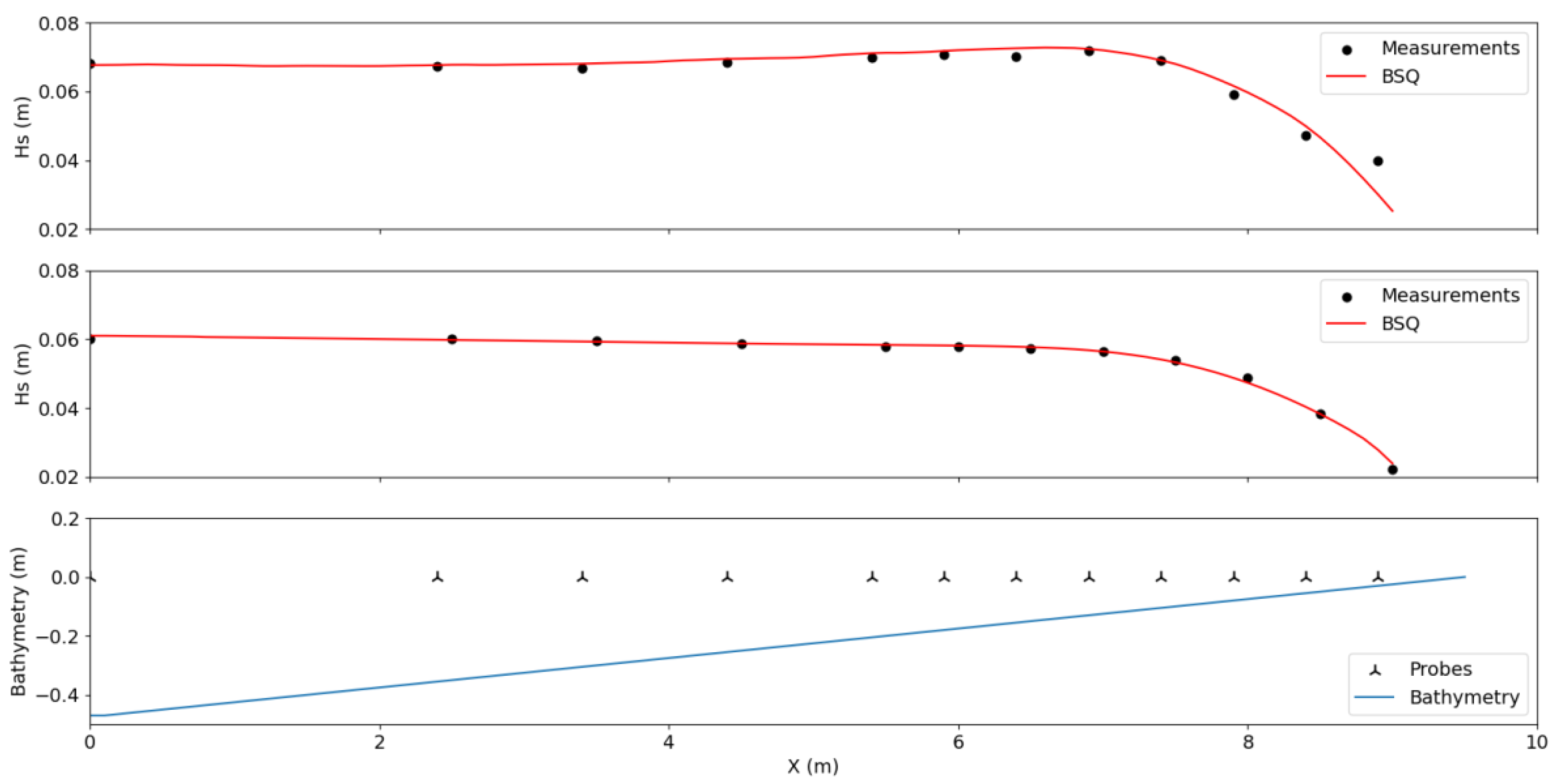
The test cases presented in the following section concern experiments on wave transformation and breaking on a plane sloping beach characterized with an impermeable slope of 1 : 20 conducted by [32]. In the experiments, irregular unidirectional waves were generated using a Pierson–Moskowitz spectrum source function. In particular, two series of tests were conducted; one utilizing a spectrum with peak frequency ${\mathrm{f}}_{\mathrm{p}} = 0.6$ (Case 1), and a second one with a peak frequency ${\mathrm{f}}_{\mathrm{p}} = 1.0$ (Case 2). In the experimental layout, waves propagate for 10 m on a bed with constant water depth of 0.47 m, before propagating up a sloped beach starting at x = 0 m. The free surface was measured by 12 probes located at 0, 2.4, 3.4, 4.4, 5.4, 5.9, 6.4, 6.9, 7.4, 7.9, 8.4, and 8.9 m, respectively. The scope of the experimental tests was to investigate wave breaking on a mildly sloping beach for unidirectional wave fields, which will serve as an important verification of the wave energy dissipation mechanisms employed in the numerical model to simulate bathymetric breaking.

Both cases were simulated with the BSQ numerical model by discretizing the bathymetry through a regular grid of spatial step of 0.1 m in both the cross-shore and alongshore directions. The wave energy spectrum was discretized using 25 frequencies, with a minimum frequency (${\mathrm{f}}_{min}$) of 0.1 Hz and a maximum frequency (${\mathrm{f}}_{max}$) of 2.5 Hz. The total simulation time was set at 160 s, with a time step of 0.0025 s to ensure numerical stability. Results of the simulated significant wave heights (${\mathrm{H}}_{\mathrm{s}}$) along the measuring locations for Case 1 and 2 of are depicted in Figure 1 and compared to the experimental measurements of [32]. At the bottom of the same Figure, the bathymetry of the experiments, along with the relative positions of the measuring probes, are showcased.

From Figure 1 above, it can be deduced that an excellent agreement is obtained between model results and experimental measurements for both test cases simulated, validating the ability of the model in reproducing accurately the wave energy dissipation rates for irregular wave fields for the case of spilling breakers (Case 1), as well as plunging breakers (Case 2). This case is of significant importance since it shows the capability of the newly added irregular wave generation source function (which has been incorporated in the enhanced version of the model developed during this research) to function smoothly in tandem with the existing wave energy dissipation mechanism. 3.2. Irregular wave propagation over a shoal (Vincent and Briggs, 1989).

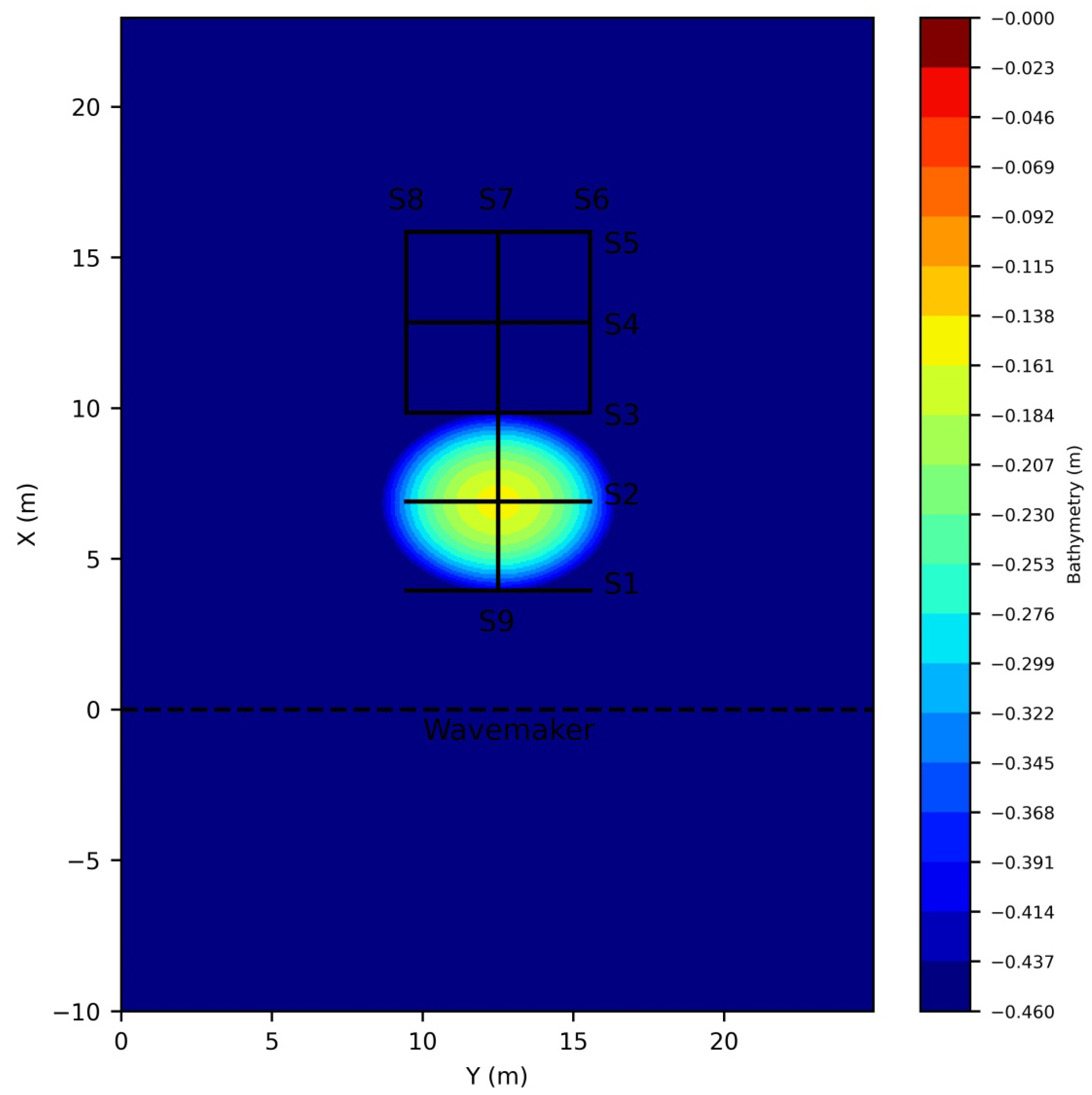
The authors in [33] performed experiments on monochromatic and random wave propagation and transformation over a submerged elliptic shoal. The experiments were conducted in the U.S. Army Coastal Engineering Research Center’s in Vicksburg, MS, USA, 29 m long by 35 m wide directional wave basin. The shoal was characterized by a major radius of 3.96 m, a minor radius of 3.05 m with a minimum water depth of approximately 0.15 m at the top, while the depth at the region outside the shoal was kept constant at 0.457 m. Several tests were performed, including the generation of unidirectional and multidirectional irregular waves utilizing a TMA spectrum [28]. The temporal evolution of the surface elevation was measured using an array of nine parallel-wire resistance-type sensors. The layout of the bathymetry along with the control sections where wave characteristics were measured is depicted in Figure 2.

In total 17 test cases were reported in [33] covering a wide range of both non-breaking and breaking wave conditions. Firstly, a series of five initial tests corresponding to non-breaking monochromatic and irregular multidirectional waves with broad and narrow directional spreading were performed. Nine tests of non-breaking waves consisting of monochromatic, unidirectional and multidirectional waves followed the initial tests. Lastly, three series of tests concerning waves breaking over the shoal for monochromatic and multidirectional random waves were conducted. In the present paper, the cases denoted as N1 and B1 in [33] corresponding to random wave propagation with narrow and broad directional spreading respectively, were reproduced utilizing the BSQ wave model. The incident wave conditions for each test are shown in

Table 1. Incident wave conditions and spectrum parametrization for the two cases in Vincent and Briggs, 1989, simulated with the BSQ wave model.

Case	Ho (cm)	Tp (s)	α	Γ	σ (˚)
N1	7.75	1.30	0.0144	2	10
B1	7.75	1.30	0.0144	2	30

. Validating model results in this experimental setup is extremely important in assessing the capability of the model to capture the wave propagation and transformation in environments were the combined effect of diffraction and refraction is dominant.

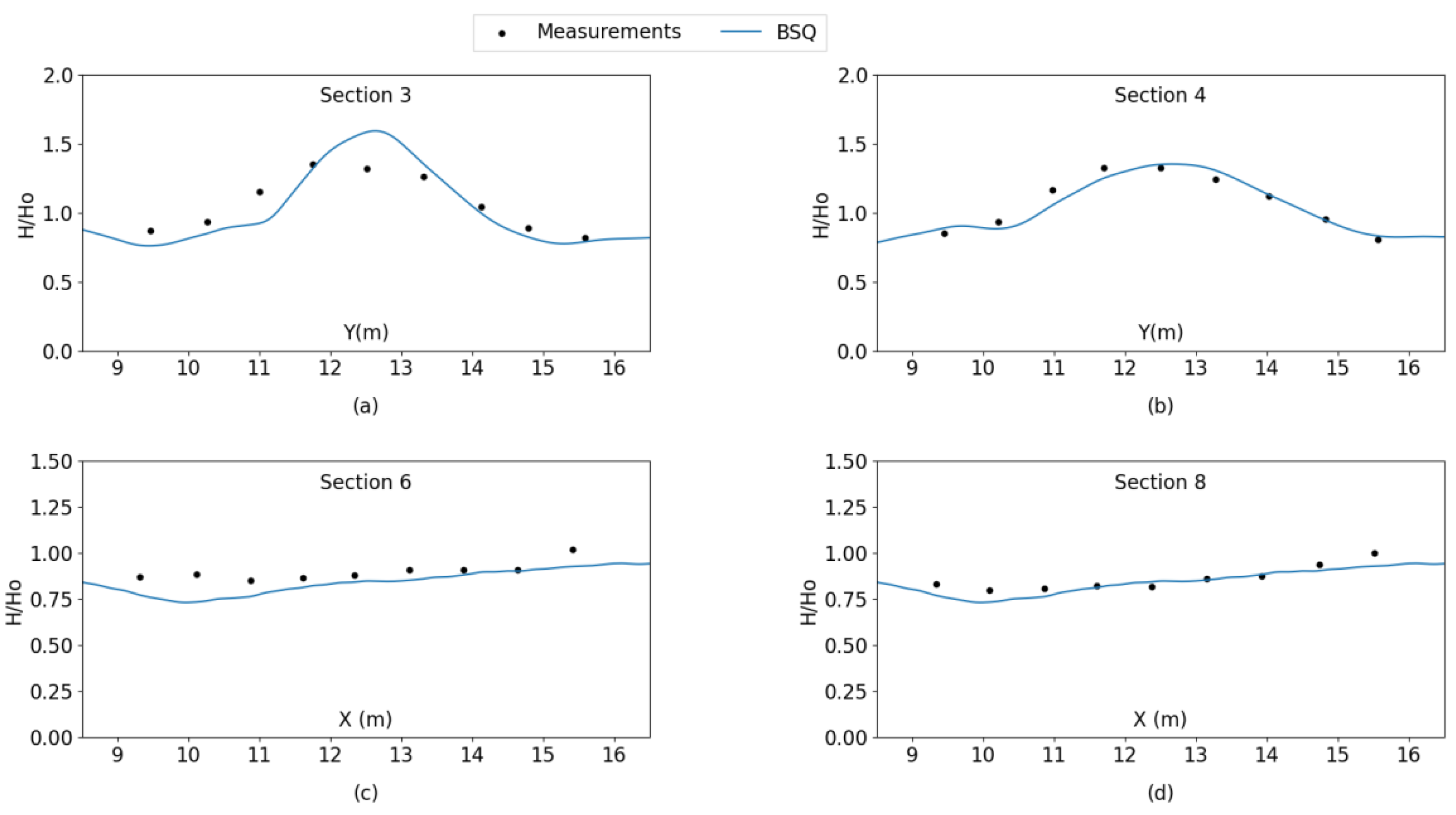
The computational grid was discretized utilizing a spatial step in both directions of Δx = Δy = 0.05 m and a time step of Δt = 0.01 s. The model was executed for 80 s and the last 5 periods were used to extract the numerical results of wave heights. For case N1, corresponding to a TMA spectrum with narrow directional spreading, comparisons between model results and experimental measurements concerning normalized wave heights (${\mathrm{H}/\mathrm{H}}_{\mathrm{o}}$) at the Sections 3,4,6 and 8 are shown in Figure 3a–d respectively.

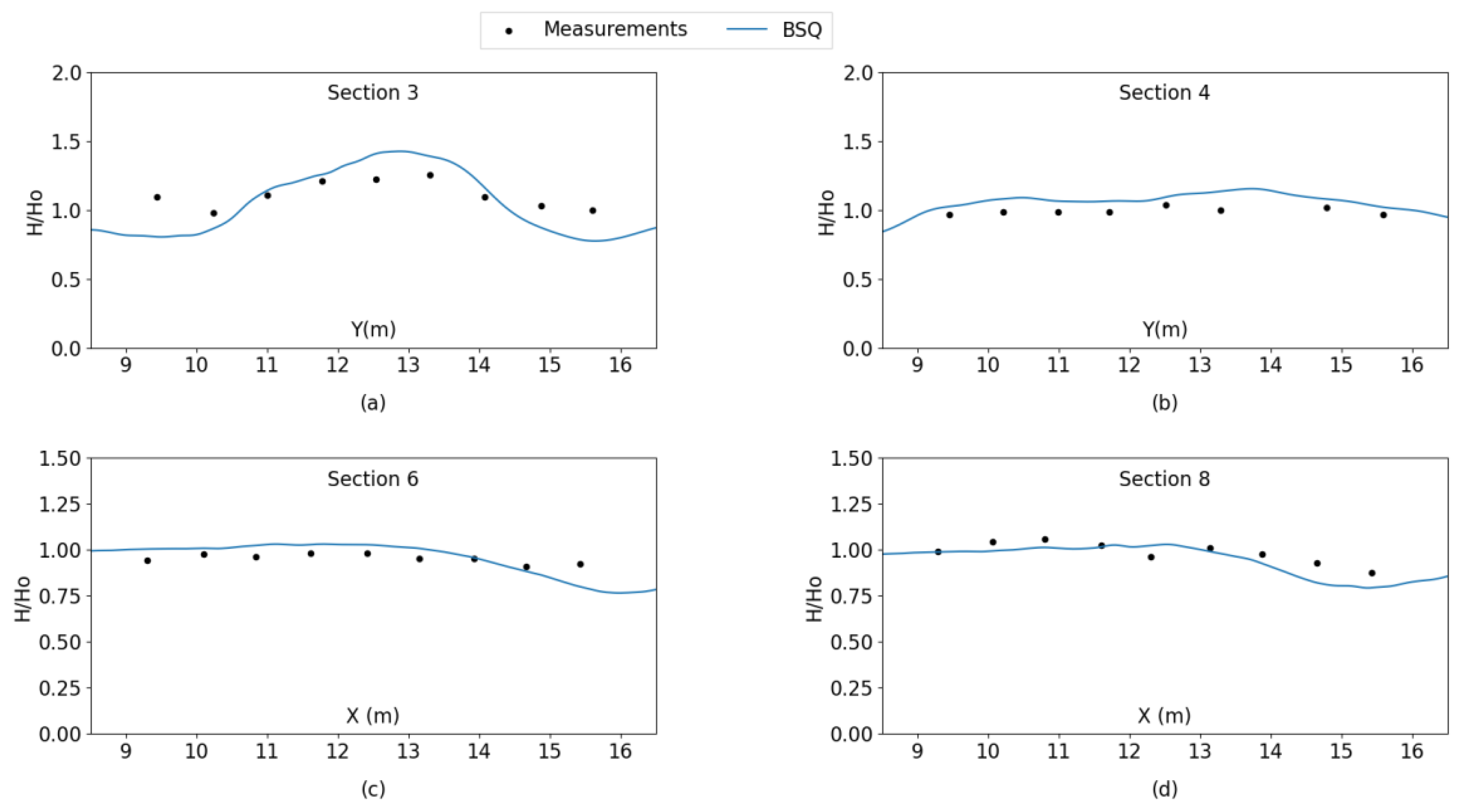
Accordingly, model results corresponding to case B1 which refers to random waves with a broad directional spreading are depicted and compared to the experimental measurements in Figure 4.

Overall, a satisfactory agreement is observed between model results and measurements for both cases shown above, validating the ability of the BSQ wave model in accurately simulating the propagation of irregular multidirectional waves under the effect of combined refraction/diffraction.

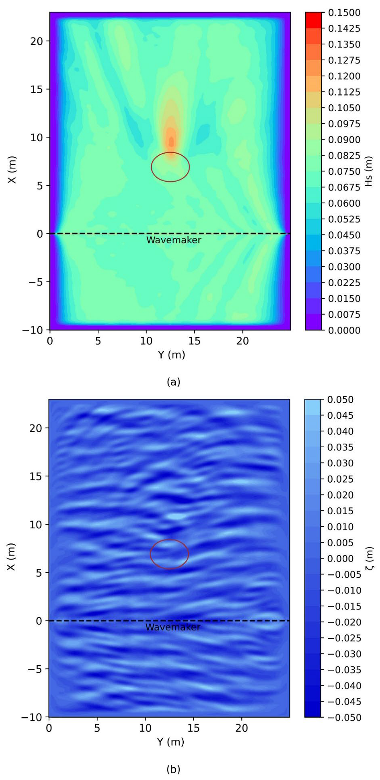
To further assess the capability of the BSQ wave model to adequately simulate the combined effect of refraction/diffraction the instantaneous wave field as well as the surface elevation obtained at the last time step is also showcased in Figure 5a,b. The obtained results are further discussed and analyzed in Section 4.

3.2. Irregular Wave Diffraction through a Breakwater Gap (Yu et al., 2000)

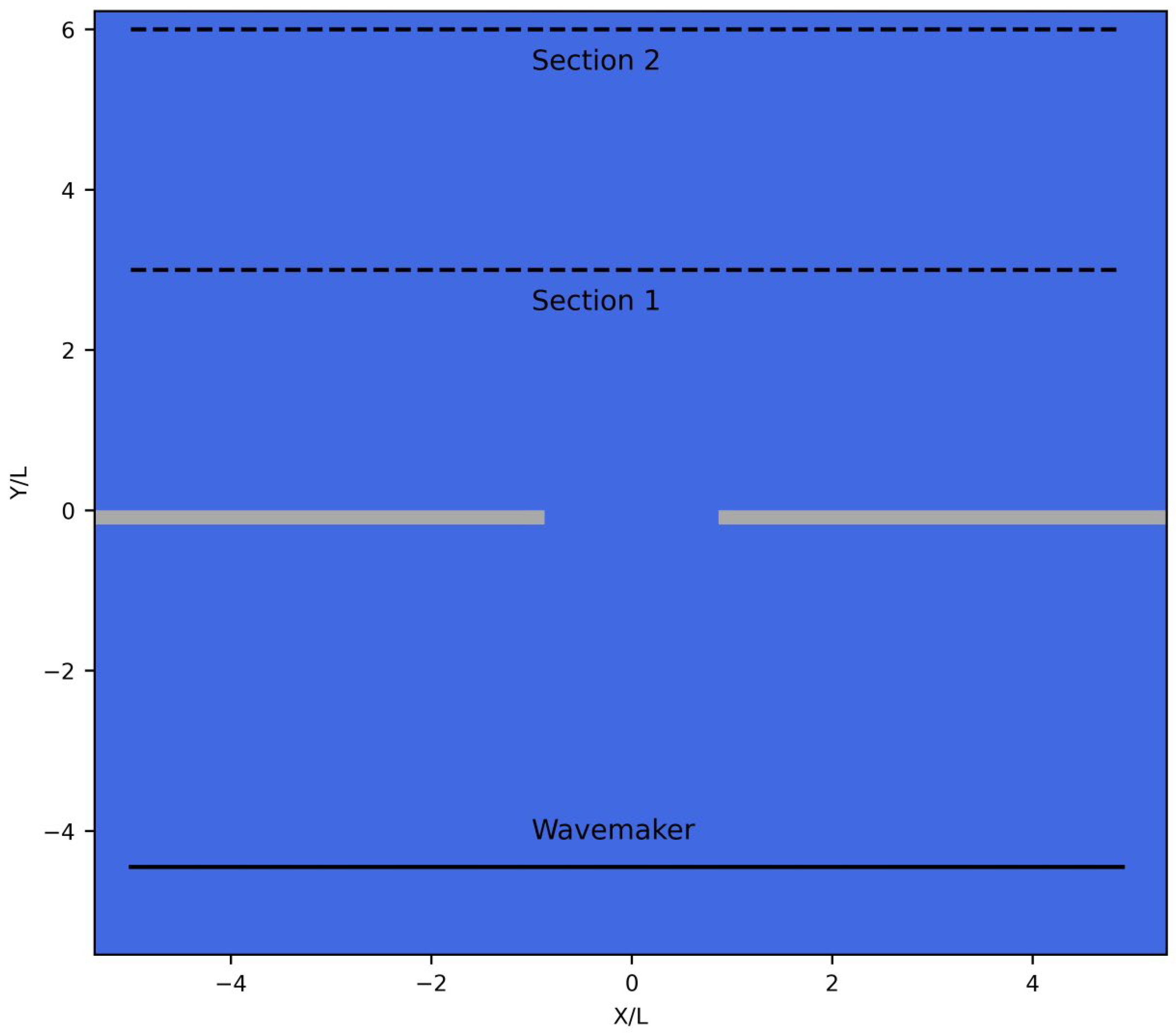
Yu et al. [34] conducted a series of experiments on wave diffraction though a breakwater gap. The experiments were carried out at the 55 m long, 34 m wide and 1.3 m deep wave basin at the Dalian University of Technology, Dalian, China. The breakwater was placed parallel to the wavemaker and at a distance measuring 7 m from the position of the wavemaker. The depth was kept constant at 0.4 m throughout the domain. The thickness of the breakwater was 0.35 m, with a gap at the center formed by two semi-circular tips. Two alternative gap widths of 3.92 m and 7.85 m were examined in the experiments. Absorbing layers 0.8 m wide were placed at waveward side of the breakwater (except from a small area around the circular tips) in order to minimize wave reflection. Several angles of wave attack in relation to the breakwater’s placement (i.e., 90°, 75°, 60° and 45°) were considered to assess the effect of diffraction in a thorough manner. Wave heights were extracted at two cross sections parallel to the breakwater and at a normalized distance of $\mathrm{Y}/\mathrm{L}$= 3.0 (Section 1) and $\mathrm{Y}/\mathrm{L}$= 6.0 (Section 2) shoreward the breakwater, (with $L$ being the wavelength corresponding to the wave peak period). The cross sections, along with the experimental layout and bathymetry, are illustrated in Figure 6.

In total, 16 test cases for each incident wave direction were carried out corresponding to monochromatic, random unidirectional or multidirectional wave conditions with broad and narrow directional spreading. Numerical validation of the BSQ wave model was carried out for the breakwater forming a gap of 3.92 m, with a wave incidence of 90° (direct wave attack) and 45° (oblique wave attack), and for the cases of random unidirectional and multidirectional waves, with a broad and narrow directional spreading, respectively. The generated waves are obtained through a Jonswap source function. An overview of the test cases reproduced in the numerical model is given in

Table 2. Incident wave conditions and spectrum parametrization for the six cases in Yu et al. 2000, simulated with the BSQ wave model.

Case	${\mathbf{H}}_{\mathbf{o}}(\mathbf{cm})$	${\mathbf{T}}_{\mathbf{p}}\left(\mathbf{s}\right)$	${\mathit{\theta }}_{\mathit{o}}(˚)$	α	Γ	s
U1	5.0	1.20	90	0.0081	4	-
N1	5.0	1.20	90	0.0081	4	19
B1	5.0	1.20	90	0.0081	4	6
U2	5.0	1.20	45	0.0081	4	-
N2	5.0	1.20	45	0.0081	4	19
B2	5.0	1.20	45	0.0081	4	6

.

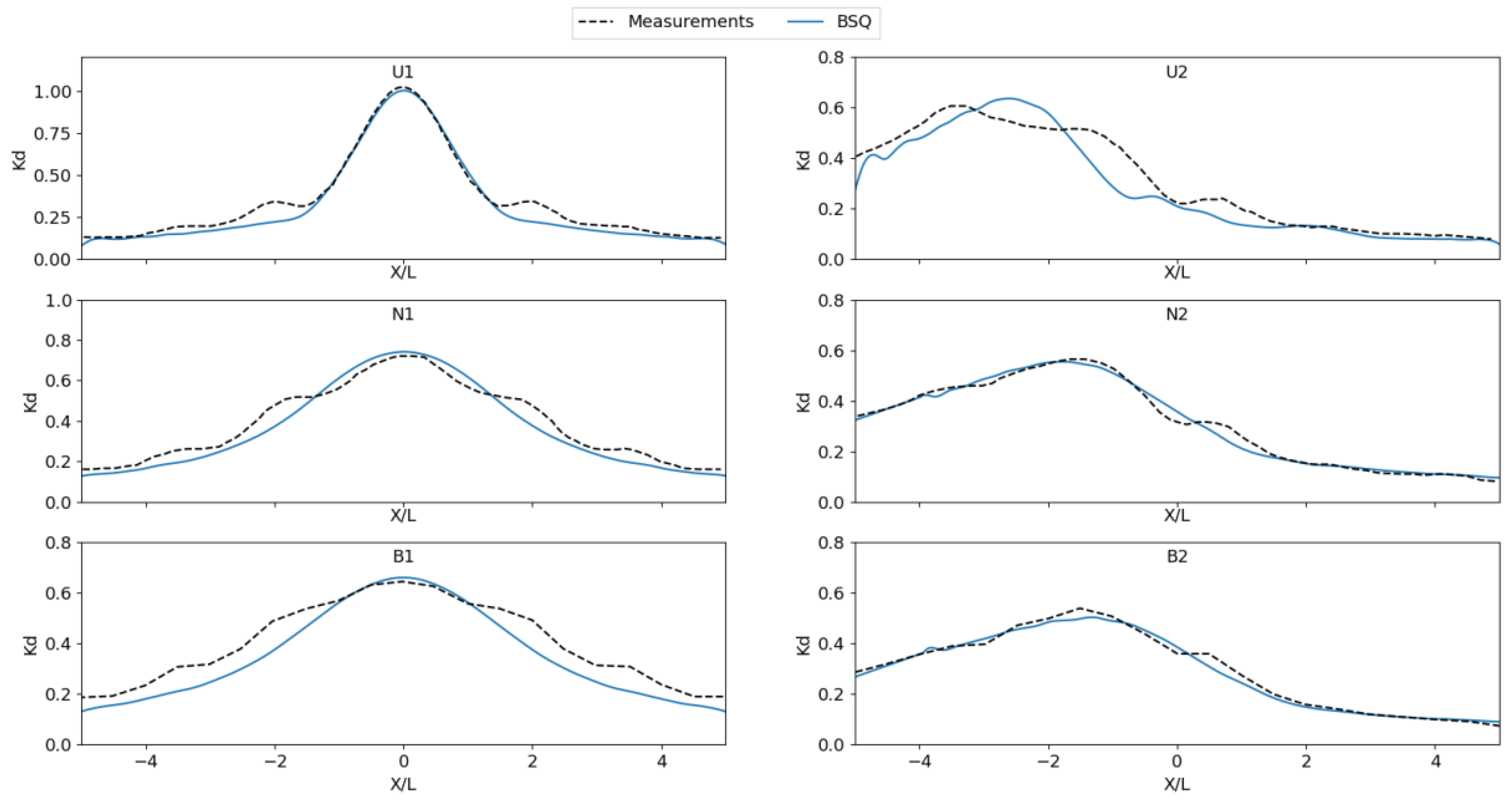
The computational grid was discretized utilizing a spatial step in both directions of Δx = Δy = 0.05 m and a time step of Δt = 0.01 s. The model was executed for 150 s, and the last 5 periods were used to extract the numerical results of wave heights. Model results concerning diffraction coefficients (${\mathrm{K}}_{\mathrm{d} }{= \mathrm{H}/\mathrm{H}}_{\mathrm{o}}$) along Section 1 are showcased in Figure 7.

Overall, a satisfactory agreement is obtained between model results and experimental measurements for all cases shown above, with the biggest discrepancies observed in the case of oblique wave attack for the unidirectional wave case. All in all, the BSQ wave model seems capable of accurately simulating the effect of wave diffraction through a breakwater gap, therefore it is rendered capable to accurately simulate wave transformation and propagation inside port basins.

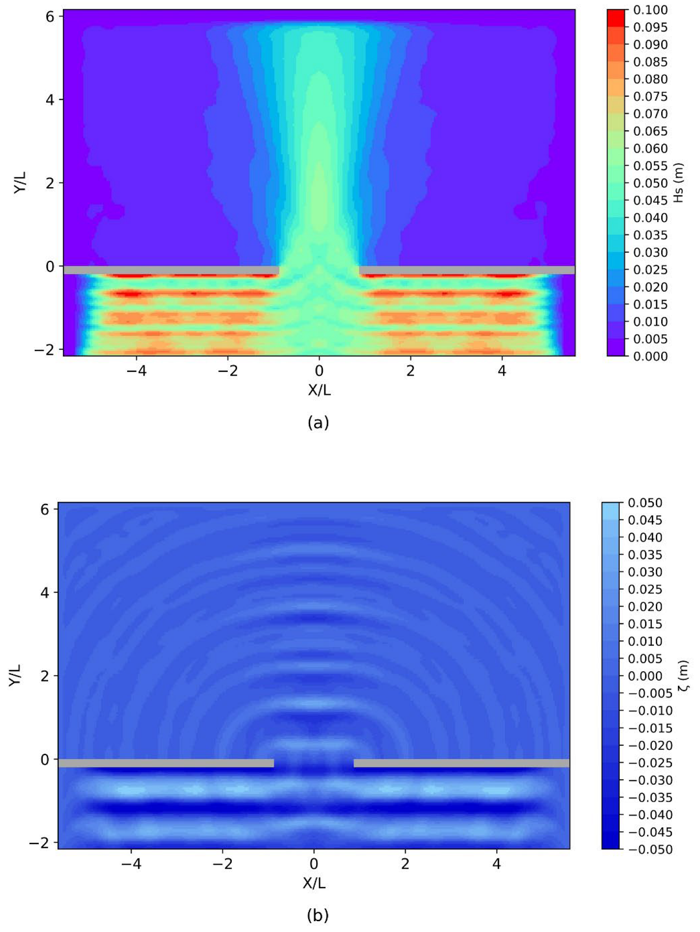
In order to provide a better overview of the wave transformation processes and the BSQ model’s capability to reproduce the effect of diffraction through a breakwater gap, the instantaneous spatial distribution of the significant wave height, as well as the free surface elevation obtained through the numerical model simulation for case U1, are showcased in Figure 8a,b The results are further discussed and analyzed in Section 4.

3.3. Wave Overtopping on a Smooth Sloping or Vertical Breakwater (Williams et al., 2019)

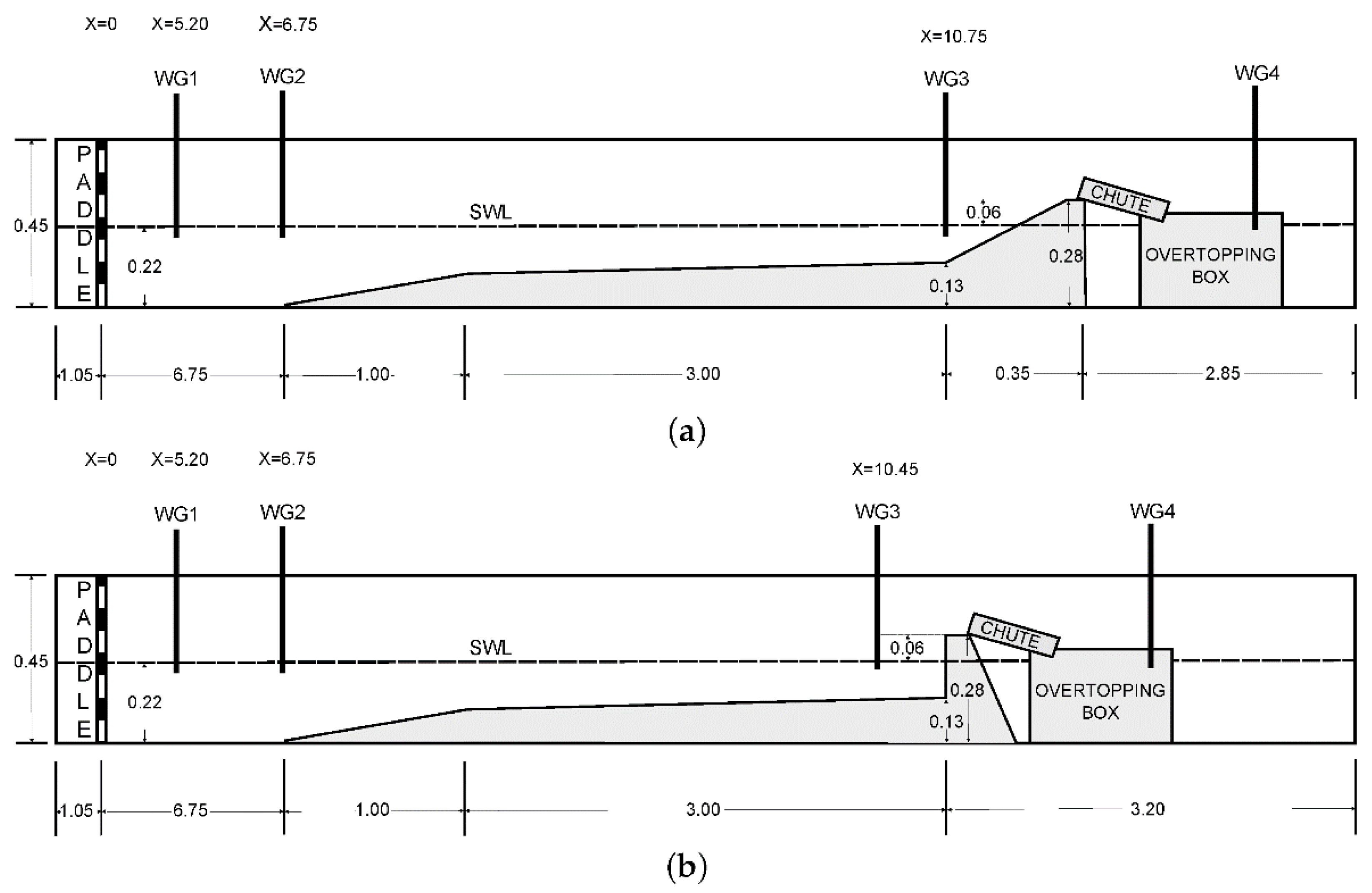
In the following section, the experiments of wave overtopping over an emerged smooth sloping breakwater or a vertical wall reported in [35] were reproduced with the BSQ wave model to evaluate its capability to estimate wave overtopping discharge at the lee of coastal protection structures. The experiments were conducted in the wave flume at the University of Nottingham, Nottingham, UK, which is approximately 15 m long and 0.23 m wide, with an operating depth of up to 0.22 m. The bottom of the flume was flat, but for the purpose of these experiments, a stainless-steel foreshore was placed, starting at x = 6.75 m from the position of the piston-type wavemaker at x = 0 m. Two different structure configurations were tested, namely a smooth sloping structure with a gradient of 1:255 and a vertical wall for the second series of tests. Both structures were characterized with an identical freeboard (${\mathrm{R}}_{\mathrm{c}}$ = 0.06). The experimental layout for both configurations is depicted in Figure 9.

A variety of incident wave conditions were generated at the wavemaker (4 distinct tests for each structure configuration) to ensure a wide range of overtopping magnitudes. Three series of wave conditions were initially tested during the experimental procedure, namely TS01, TS02 and TS05, which were deemed suitable for both the structure geometries, and were therefore tested. Due to the differing wave-structure interaction for each configuration, the fourth wave condition for each case varied. For the smooth slope, a combination of wave characteristics that lead to low overtopping volumes (TS03) was chosen; however, this resulted in no overtopping of the vertical wall structure, and therefore, it could not be used for this configuration. Instead, a more energetic wave condition was chosen for the vertical structure only (TS07). Waves were generated through a Jonswap spectrum source function, with a peak factor of $\mathsf{\gamma }$ = 3.3, for all the test cases examined. A compiled list of the incident wave conditions of each test case that was reproduced with the BSQ wave model is showcased in

Table 3. Incident wave conditions and spectrum parametrization for the two cases in Williams et al., 2019, simulated with the BSQ wave model.

Case	Structure Type	Hmo,i (cm)	Tp (s)	Rc (cm)	Rc/Hmo,i (-)
TS01-SS	Smooth Sloping	6.0	1.01	6.0	1.00
TS05-SS	Smooth Sloping	5.0	0.93	6.0	1.20
TS02-SS	Smooth Sloping	4.0	0.86	6.0	1.50
TS03-SS	Smooth Sloping	3.0	0.70	6.0	2.00
TS01-VW	Vertical Wall	6.0	1.01	6.0	1.00
TS07-VW	Vertical Wall	5.0	1.24	6.0	1.20
TS05-VW	Vertical Wall	5.0	0.93	6.0	1.20
TS02-VW	Vertical Wall	4.0	0.86	6.0	1.50

.

For the case of the vertical structure, a fully reflecting boundary at the wall’s face was considered, whereas for the smooth structure, an additional constant eddy viscosity coefficient (${\mathrm{v}}_{\mathrm{h}} = 0.01$) was specified to emulate partial reflection along the slope. In order to obtain incident wave conditions at the structure’s toe wave averaging of the surface elevation signal at the wave model was carried out at a time interval spanning between the time step corresponding to the arrival of the peak period wave components and up until the “first wave” reaches the face of the structure, signifying the initiation of wave reflection. For the case of the smooth sloping structure, bottom scattering is expected to occur as waves propagate along the structures toe, which may inadvertently influence the incident wave at the structure’s toe. The total model run-time for all simulations was set at 41.0 s.

The obtained results concern the computed spectral wave height at the toe of the structure ${\mathrm{H}}_{mo,\mathrm{c}}$ (at the position of WG3 of Figure 9), along with the calculated normalized wave overtopping discharge ${\mathrm{Q}}_{*,\mathrm{c}}$. For the calculation of the overtopping discharge, Equation (21) was utilized for the case of the smooth sloping structure, whereas Equation (22) was implemented for the case of the vertical wall. In order to quantify the difference between the measured and computed values, the absolute relative difference between each measured quantity (${\mathrm{X}}_{\mathrm{m}}$) and the computed one (${\mathrm{X}}_{\mathrm{c}}$) was obtained through the following relationship:

$${\mathrm{X}}_{diff} = \frac{\left|{\mathrm{X}}_{\mathrm{m}} - {\mathrm{X}}_{\mathrm{c}}\right|}{{\mathrm{X}}_{\mathrm{m}}}$$

(24)

The computed and measured values concerning wave heights at the toe of the structure and normalized overtopping discharge along with the corresponding absolute relative difference for each quantity are shown in

Table 4. Incident wave conditions and spectrum parametrization for the six cases in Williams et al., 2019, simulated with the BSQ wave model.

Case	Hmo,m (cm)	Hmo,c (cm)	Hmo,diff (%)	Q*,m (-)	Q*,c (cm)	Q*,diff (%)
TS01-SS	4.30	4.36	1.44%	0.008655	0.006929	19.94%
TS05-SS	3.80	3.92	3.22%	0.005362	0.004739	11.62%
TS02-SS	3.20	3.33	4.06%	0.00233	0.002358	1.20%
TS03-SS	2.00	1.98	1.17%	0.000543	0.000069	87.30%
TS01-VW	4.30	4.24	1.42%	0.004571	0.00098	78.62%
TS07-VW	4.00	4.07	1.70%	0.004268	0.00083	80.59%
TS05-VW	3.80	3.72	2.11%	0.002192	0.00056	74.24%
TS02-VW	3.20	3.22	0.51%	0.00082	0.00028	65.91%

.

As shown in Table 4, the prediction error for the computed incident wave heights at the toe of the structure is relatively small, validating the use of the “parametric simplified” methodology for the purpose of distinguishing incident wave conditions from the reflected ones. Larger prediction errors can be observed for the case of the smooth sloping structure, which can be attributed to the inherent presence of bottom scattering in the governing equation. On the other hand, the prediction errors of the normalized overtopping discharge are significantly larger, especially for the case of the vertical wall. Taking into account that the errors in the calculated wave heights are minimal, the errors in the calculation of overtopping discharges stem from the utilization of the empirical formulae employed to calculate the wave overtopping discharges. Although the relative error is quite significant at first sight, each test falls within the 90% confidence band of the empirical formulae, as specified in [30], and further clarified in [35]. Therefore, the performance of each empirical relationship depends on the structure’s configuration (the empirical method for smooth sloping structures performs generally better than the vertical wall), as well as on the total volume of overtopping and the severity of the event, as stated in [35]. From the above, given the minimal computational effort required by the integration of the empirical calculation formulae for wave overtopping, as well as the acceptable accuracy of the obtained results, the BSQ model is deemed to perform quite satisfactorily in predicting the wave overtopping discharge for a variety of incident wave conditions and structure configurations.

4. Discussion

In the previous section, an extensive validation of the BSQ wave model was provided, in order to access the capability of the wave model to deal with the propagation of irregular waves in the coastal zone, with or without the presence of coastal protection structures.

Wave breaking of unidirectional waves was investigated by reproducing the experiments of [32]. It can be seen from Figure 1 that the model predicts the shoaling and subsequent decay, due to wave breaking fairly well. For Case 1 of [32], corresponding to a peak frequency ${\mathrm{f}}_{\mathrm{p}}$ = 0.6 Hz, a small discrepancy between measurements and model results can be observed in the wave stations close to the shoreline. This can be attributed to the underprediction of the wave setup magnitude in the wave model. For Case 2 of [32], which corresponds to a peak frequency of ${\mathrm{f}}_{\mathrm{p}}$ = 1.0 Hz, model results are almost identical to the experimental measurements, validating the capability of the model to predict the onset of breaking as well as the magnitude of wave energy dissipation on a plane sloping beach in a very accurate manner.

The second case serves the purpose of evaluating the propagation of irregular multidirectional wave fields over an elliptic shoal under the combined effect of wave refraction-diffraction [33]. It can be deduced from Figure 3 that the model results are in very satisfactory agreement with the experimental measurements when examining the propagation of irregular multidirectional waves of a narrow directional spreading. The biggest discrepancy can be observed in Section 3. In particular, a higher peak and focusing of wave energy can be observed at Y = 12.5 m in the model results of normalized wave height. This can be attributed to an overestimation of wave refraction/diffraction in the numerical model for the particular Section, since it is located at the northern end of the shoal. Conversely, the agreement is excellent on Section 4, which is located further away from the shoal, capturing the transformation of the wave height due to the refraction and diffraction of wave rays in a very satisfying manner. The same holds true for the transverse Sections 6 and 8, where the performance of the wave model is excellent compared to the measured values. For the propagation of irregular multidirectional waves with a broad directional spreading, model results are deemed very satisfactory. In particular, due to the broad directional spreading, the normalized wave height variations, especially along Sections 3 and 4, have smoother peaks, and are smaller in magnitude. In accordance to the conclusions drawn for the case of narrow directional spreading, the biggest discrepancy is observed once again in Section 3, with a sharper peak being present in model results due to the increased effect of wave diffraction from the shoal. It should be noted that selecting few wave directional divisions can lead to a deterioration of model results associated with an inadequate resolution of the wave directional spreading function for the single summation method of spectrum discretization. Specifying a number of wave directional divisions at a number from 13–26 was deemed accurate for the particular test case, and led to accurate results for all cases examined. All in all, the BSQ wave model is considered to reproduce the combined effect of refraction/diffraction in a very adequate manner.

The third validation case concerned the propagation of irregular unidirectional and multidirectional waves through a breakwater gap [34]. This test case is of paramount importance, since it serves as a thorough evaluation of the wave-structure interaction mechanisms present in the BSQ wave model. Cases of direct and oblique wave attack were simulated with the wave model for a variety of incident wave conditions concerning unidirectional and multidirectional wave fields with narrow and broad directional spreading, respectively. For the case of perpendicular wave propagation in relation to the breakwater gap, a satisfactory agreement is achieved for all cases of incident waves. More specifically, for the unidirectional wave case (U1), the normalized wave heights are in good agreement with respect to the magnitude of the experimental measurements, as can be seen from Figure 7. A small underestimation of the diffraction coefficient behind the tips of the breakwater can be observed in Section 1 (at X/L = −2.0 and X/L = 2.0), with secondary peaks being present in the experimental measurements. This underestimation can also be observed in tests N1 and B1, and can be attributed to the difference of the absorbing layer between the model and experiment, leading to different patterns of wave reflection from the tip of the breakwater. This is particularly evident in case U2, where a difference at the location of the peak of the diffraction coefficient is observed, due to the increased presence of reflected waves from the tip and lee of the breakwater, which are more prevalent in the oblique wave attack cases. However, for the multidirectional wave cases (N2 and B2), the effect of wave reflection from the breakwater’s tip is not as prevalent, due to the variety of angles with which waves approach the breakwater, counterbalancing the focusing of the wave energy associated with a singular wave angle for the unidirectional wave case. In general, a very good agreement is observed between model results and experimental measurements, rendering the BSQ wave model a valuable tool for the estimation of wave agitation and propagation inside port basins.

Lastly, the experiments of [35] concerning wave overtopping over a smooth sloping structure as well as a vertical wall were reproduced with the BSQ wave model in order to evaluate its capability to predict wave overtopping discharges at the lee of the structure. The purpose of this evaluation is twofold, as firstly it is important to assess the capability of the model to predict incident wave heights at the toe of the structure by minimizing the presence of reflected waves from the boundaries in the signal. A parametric simplified methodology consisting of wave averaging between the time interval for which the peak period reaches the computational cell of the structure’s toe until the time step for which waves reach the face of the structure and are hence reflected was utilized in the context of this research. As seen in Table 4, the predicted wave heights at the toe of the structure are in good agreement with the experimental measurements for both structure configurations. The relative errors are higher for the case of smooth sloping structures, due to partial reflection as waves propagate along the structure’s slope. It should be noted that this simplified methodology is valid for the cases of narrow frequency wave spectra, as a broad spectrum can lead to an overestimation or underestimation of the incident wave heights since several wave components travel with different phase velocities. Another possibility is offered in the BSQ wave model, namely executing a “reference domain” simulation without the presence of the structure, in order to compute incident wave height at its toe, however this approach significantly increases numerical burden, especially for large computational domains. Regarding the estimation of overtopping discharges, the empirical formulae in [30] and [31] were utilized for the smooth sloping breakwater and vertical wall, respectively. The relative difference between measurements and model predictions are quite significant, especially for the case of vertical breakwaters. This difference is dependent on the magnitude of overtopping volumes (i.e., higher discrepancies are observed for the smooth sloping structure for TS03-SS, which corresponds to low overtopping discharge). This can be caused by the fact that the formula of [30] was calibrated for the case of a small freeboard (low-crested structure configuration), which is not the case in TS03-SS [35]. For all cases examined though, the obtained results lie well within the confidence intervals of the empirical methods [35]. Taking all the above into account, it is considered that the methodology to calculate wave overtopping in the BSQ wave model offers a very good compromise between accuracy, simulation efficiency, and speed.

5. Conclusions

In the present paper, a highly nonlinear Boussinesq wave model (BSQ) initially developed by [18] and later extended by [19] to account for wave propagation over submerged porous mediums was presented. The model was further extended to incorporate the estimation of wave overtopping discharges at the lee of coastal protection works utilizing an ad hoc incorporation of empirical relationships [30,31]. The model has been thoroughly validated against four series of experiments covering a wide range of coastal engineering applications, namely irregular wave breaking on a plane beach [32], wave propagation over a shoal [33], wave penetration through a breakwater gap [34] and wave overtopping at the lee of a breakwater [35]. For all the test cases, examined model results were in very good agreement with the experimental measurements.

The first case simulated with the BSQ model concerned irregular wave breaking on a plane sloping beach, as presented in [32]. Model results were in excellent agreement with experimental measurements, providing an accurate estimation of wave energy dissipation, due to bathymetric breaking for both the cases of spilling and plunging breakers.

For the next experiment of [33], which was reproduced with the wave model, the obtained results were in excellent agreement with the experimental measurements for the case of irregular multidirectional wave propagation over a submerged shoal with narrow and broad directional spreading, respectively. The focusing of wave energy behind the shoal was adequately captured, validating the capability of the wave model to simulate the combined effect of refraction/diffraction, due to its improved dispersion characteristics. A slight overestimation of wave heights was observed at Section 3, which was positioned directly behind the submerged shoal.

In the penultimate case, the model’s capability to simulate wave penetration through a breakwater gap, as presented in [34], was investigated. Diffraction coefficients obtained by the numerical model simulations for the cases of unidirectional and multidirectional wave fields with narrow and broad directional spreading respectively, were in general in a very good agreement with the experimental measurements. The wave agitation at the lee of the breakwater was also predicted quite satisfactorily by the numerical model. Some small discrepancies between measurements and model predictions can be attributed to the different absorbing layers’ characteristics present in the experimental layout and the numerical model, leading to the presence of reflected waves, which influence the results, especially for the case of oblique wave attack of unidirectional waves.

Lastly, the experiments of [35] concerning wave overtopping on a smooth sloping structure or a vertical wall were simulated with the BSQ model. An ad hoc “simplified parametric” methodology to distinguish incident wave heights from reflected ones was proven to be adequate to provide an efficient and accurate estimation of the incident wave heights at the toe of the structure. Differences between the calculated and measured overtopping discharges were larger, in particular for the case of vertical wall, however the results were well within the confidence intervals of the empirical formulations [35]. Given the computational efficiency of integrating the empirical overtopping formulae in the model formulations, this addition is considered valuable in providing calculations of wave overtopping for various incident wave conditions and structure configurations with respectable accuracy.

Taking into consideration the extensive validation of the BSQ wave model presented herein, it is considered to be capable of accurately simulating the complex wave transformation processes taking place in the coastal zone, with or without the presence of coastal protection works, as well as inside wave basins. Therefore, the model is rendered to be a valuable tool at the disposal of coastal engineers and scientists desiring to obtain accurate solutions on wave propagation in complex domains, and for a variety of incident wave conditions at reasonable computations times.

Regarding possible future research aspects and developments, the generalization of the numerical solution to a curvilinear coordinate system as described in [36] is to be undertaken, in order to better describe complex and curved geometries such as shorelines and coastal defense structures. Furthermore, the inclusion of ship-borne wakes in the BSQ wave model [37], as well as their subsequent interaction with coastal structures, can further enhance the computation of wave agitation inside port basins.

References

- Holthuijsen, L.H. Waves in Oceanic and Coastal Waters; Cambridge University Press: Cambridge, UK, 2007. [Google Scholar]
- Pachang, V.; Wei, G.; Pearce, R.; Briggs, M. Numerical simulation of irregular wave propagation over a shoal. J. Waterw. Port. Coast. Ocean. Eng. 1990, 116, 324–340. [Google Scholar] [CrossRef]
- Chawla, A.; Özkan-Haller, H.T.; Kirby, J.T. Spectral Model for Wave Transformation and Breaking over Irregular Bathymetry. J. Waterw. Port Coastal Ocean Eng. 1998, 124, 189–198. [Google Scholar] [CrossRef]
- Chondros, M.; Metallinos, A.; Memos, C.; Karambas, T.; Papadimitriou, A. Concerted nonlinear mild-slope wave models for enhanced simulation of coastal processes. Appl. Math. Model. 2021, 91, 508–529. [Google Scholar] [CrossRef]
- Peregrine, D.H. Long waves on a beach. J. Fluid Mech. 1967, 27, 815–827. [Google Scholar] [CrossRef]
- Wei, G.; Kirby, J. Time-Dependent Numerical Code for Extended Boussinesq Equations. J. Waterw. Port. Coast. Ocean. Eng. 1995, 121, 251–261. [Google Scholar] [CrossRef]
- Karambas, T.V.; Memos, C.D. Boussinesq Model for Weakly Nonlinear Fully Dispersive Water Waves. J. Waterw. Port Coast. Ocean Eng. 2009, 135, 187–199. [Google Scholar] [CrossRef]
- Li, B. Wave Equations for Regular and Irregular Water Wave Propagation. J. Waterw. Port Coast. Ocean Eng. 2008, 134, 121–142. [Google Scholar] [CrossRef]
- Serre, F. Contribution à l’étude des écoulements permanents et variables dans les canaux. La Houille Blanche 1953, 39, 374–388. [Google Scholar] [CrossRef] [Green Version]
- Green, A.E.; Naghdi, P.M. A derivation of equations for wave propagation in water of variable depth. J. Fluid Mech. 1976, 78, 237–246. [Google Scholar] [CrossRef]
- Zelt, J. The run-up of nonbreaking and breaking solitary waves. Coast. Eng. 1991, 15, 205–246. [Google Scholar] [CrossRef]
- Karambas, T.; Koutitas, C. A breaking wave propagation model based on the Boussinesq equations. Coast. Eng. 1992, 18, 1–19. [Google Scholar] [CrossRef]
- Schäffer, H.A.; Madsen, P.A.; Deigaard, R. A Boussinesq model for waves breaking in shallow water. Coast. Eng. 1993, 20, 185–202. [Google Scholar] [CrossRef]
- Madsen, P.; Sørensen, O.; Schäffer, H. Surf zone dynamics simulated by a Boussinesq type model. Part I. Model description and cross-shore motion of regular waves. Coast. Eng. 1997, 32, 255–287. [Google Scholar] [CrossRef]
- Nwogu, O. Alternative Form of Boussinesq Equations for Nearshore Wave Propagation. J. Waterw. Port Coast. Ocean Eng. 1993, 119, 618–638. [Google Scholar] [CrossRef] [Green Version]
- Madsen, P.A.; Schäffer, H.A. Higher–Order Boussinesq–Type equations for surface gravity waves: Derivation and analysis. Philos. Trans. R. Soc. A Math. Phys. Eng. Sci. 1998, 356, 3123–3181. [Google Scholar] [CrossRef]
- Schäffer, H.A. Another step towards a post-Boussinesq wave model. In Proceedings of the 29th International Conference on Coastal Engineering, Lisbon, Portugal, 19–24 September 2004. [Google Scholar]
- Chondros, M.K.; Memos, C.D. A 2DH nonlinear Boussinesq-type wave model of improved dispersion, shoaling, and wave generation characteristics. Coast. Eng. 2014, 91, 99–122. [Google Scholar] [CrossRef]
- Metallinos, A.S.; Klonaris, G.; Memos, C.D.; Dimas, A. Hydrodynamic conditions in a submerged porous breakwater. Ocean Eng. 2019, 172, 712–725. [Google Scholar] [CrossRef]
- Cruz, E.; Isobe, M.; Watanabe, A. Boussinesq equations for wave transformation on porous beds. Coast. Eng. 1997, 30, 125–156. [Google Scholar] [CrossRef]
- Van Gent, M.R.A. Wave Interaction with Permeable Coastal Structures. Ph.D. Thesis, Delft University of Technology, Delft, The Netherlands, 12 December 1995. [Google Scholar]
- Sollitt, C.K.; Cross, R.H. Wave transmission through permeable breakwaters. In Proceedings of the 13th International Conference on Coastal Engineering, Vancouver, Canada, 10–14 July 1972. [Google Scholar]
- Losada, I.; Losada, M.; Martín, F. Experimental study of wave-induced flow in a porous structure. Coast. Eng. 1995, 26, 77–98. [Google Scholar] [CrossRef]
- Hsiao, S.-C.; Liu, P.; Chen, Y. Nonlinear water waves propagating over a permeable bed. Proc. R. Soc. Lond. A 2002, 458, 1291–1322. [Google Scholar] [CrossRef]
- Kennedy, A.; Chen, Q.; Kirby, J.T.; Dalrymple, R. Boussinesq Modeling of Wave Transformation, Breaking, and Runup. I: 1D. J. Waterw. Port Coast. Ocean Eng. 2000, 126, 39–47. [Google Scholar] [CrossRef] [Green Version]
- Chen, Q.; Kirby, J.; Dalrymple, R.; Kennedy, A.; Chawla, A. Boussinesq Modeling of Wave Transformation, Breaking, and Runup. II: 2D. J. Waterw. Port. Coast. Ocean. Eng. 2000, 126, 48–56. [Google Scholar] [CrossRef]
- Yu, Y.X.; Liu, S.X.; Li, L. Numerical simulation of multi-directional waves. In Proceedings of the International Society of Offshore and Polar Engineers Conference, Edinburgh, UK, 11–16 August 1991. [Google Scholar]
- Bouws, E.; Günther, H.; Rosenthal, W.; Vincent, C.L. Similarity of the wind wave spectrum in finite depth water: 1. Spectral form. J. Geophys. Res. Space Phys. 1985, 90, 975–986. [Google Scholar] [CrossRef]
- Goda, Y. Random Seas and Design of Maritime Structures, 2nd ed.; Advanced Series on Ocean Engineering; World Scientific Publishing Company: Singapore,, 2000; p. 464. [Google Scholar]
- EurOtop. Manual on Wave Overtopping of Sea Defences and Related Structures, 2nd ed.; EurOtop: Brussels, Belgium, 2018; p. 304. [Google Scholar]
- Besley, P.; Stewart, T.; Allsop, N.W.H. Overtopping of Vertical Structures: New Prediction Methods to Account for Shallow Water Conditions. In Coastlines, Structures and Breakwaters; Thomas Telford Ltd.: London, UK, 1998; pp. 46–57. [Google Scholar]
- Mase, H.; Kirby, J. Hybrid Frequency-Domain KdV Equation for Random Wave Transformation. In Proceedings of the 23rd International Conference on Coastal Engineering, Venice, Italy, 4–9 October 1992. [Google Scholar]
- Vincent, C.L.; Briggs, M.J. Refraction—Diffraction of Irregular Waves over a Mound. J. Waterw. Port Coast. Ocean Eng. 1989, 115, 269–284. [Google Scholar] [CrossRef]
- Yu, Y.-X.; Liu, S.-X.; Li, Y.; Wai, O.W. Refraction and diffraction of random waves through breakwater. Ocean Eng. 2000, 27, 489–509. [Google Scholar] [CrossRef]
- Williams, H.E.; Briganti, R.; Romano, A.; Dodd, N. Experimental Analysis of Wave Overtopping: A New Small Scale Laboratory Dataset for the Assessment of Uncertainty for Smooth Sloped and Vertical Coastal Structures. J. Mar. Sci. Eng. 2019, 7, 217. [Google Scholar] [CrossRef] [Green Version]
- Shi, F.; Dalrymple, R.; Kirby, J.; Chen, Q.; Kennedy, A. A fully nonlinear Boussinesq model in generalized curvilinear coor-dinates. Coast. Eng. 2001, 42, 337–358. [Google Scholar] [CrossRef]
- David, C.G.; Roeber, V.; Goseberg, N.; Schlurmann, T. Generation and propagation of ship-borne waves-Solutions from a Boussinesq-type model. Coast. Eng. 2017, 127, 170–187. [Google Scholar] [CrossRef] [Green Version]
Figure 1.
Computed (solid red line) and measured (circular markers) values of Case 1 (top), Case 2 (middle) for the experiments of Mase and Kirby 1992, along with the bathymetry (solid blue line) and probe positions (markers) at the bottom.
Figure 2.
Layout of the experiments of Vincent and Briggs, 1989, and control sections (S1−S9) where wave characteristics were measured.
Figure 3.
Comparison of simulated (lines) and measured (points) normalized wave heights results of case N1 of the Vincent and Briggs, 1989, experiments, (a): Section 3, (b): Section 4, (c): Section 6, (d): Section 8.
Figure 4.
Comparison of simulated (lines) and measured (points) normalized wave heights results of case B1 of the Vincent and Briggs, 1989, experiments, (a): Section 3, (b): Section 4, (c): Section 6, (d): Section 8.
Figure 5.
Instantaneous significant wave height (a) and surface elevation (b) of the case N1 of Vincent and Briggs, 1989, extracted at the end of the BSQ model simulation. The red ellipse denoted the position of the shoal.
Figure 6.
Layout of the numerical configuration of the experiments in Yu et al., 2000, with the position of Sections(dashed lines), where wave characteristics were obtained.
Figure 7.
Comparison of simulated (solid lines) and measured (dashed lines) normalized wave heights results at the cross Section 1 of the simulated cases of Yu et al., 2000, experiments.
Figure 8.
Instantaneous significant wave height (a) and surface elevation (b) of the case U1 of Yu et al., 2000, extracted at the end of the BSQ model simulation.
Figure 9.
Layout of the physical model tests (a) smooth sloping structure, (b) vertical wall (adapted from Williams et al., 2019).