Article

Error Distribution Model to Standardize LPUE, CPUE and Survey-Derived Catch Rates of Target and Non-Target Species

1
Okeanos-UAc Instituto de Investigação em Ciências do Mar, Universidade dos Açores, Rua Prof. Dr. Frederico Machado, 4, 9900-138 Horta, Faial, Portugal
2
IMAR Instituto do Mar, Departamento de Oceanografia e Pescas, Universidade dos Açores, Rua Prof. Dr. Frederico Machado, 4, 9901-862 Horta, Faial, Portugal
*
Author to whom correspondence should be addressed.
Submission received: 12 November 2021 / Revised: 16 December 2021 / Accepted: 18 December 2021 / Published: 22 December 2021
(This article belongs to the Special Issue Ocean and Coastal Modelling)

Abstract

:
Indices of abundance are usually a key input parameter used for fitting a stock assessment model, as they provide abundance estimates representative of the fraction of the stock that is vulnerable to fishing. These indices can be estimated from catches derived from fishery-dependent sources, such as catch per unit effort (CPUE) and landings per unit effort (LPUE), or from scientific survey data (e.g., relative population number—RPN). However, fluctuations in many factors (e.g., vessel size, period, area, gear) may affect the catch rates, bringing the need to evaluate the appropriateness of the statistical models for the standardization process. In this research, we analyzed different generalized linear models to select the best technique to standardize catch rates of target and non-target species from fishery dependent (CPUE and LPUE) and independent (RPN) data. The examined error distribution models were gamma, lognormal, tweedie, and hurdle models. For hurdle, positive observations were analyzed assuming a lognormal (hurdle–lognormal) or gamma (hurdle–gamma) error distribution. Based on deviance table analyses and diagnostic checks, the hurdle–lognormal was the statistical model that best satisfied the underlying characteristics of the different data sets. Finally, catch rates (CPUE, LPUE and RPN) of the thornback ray Raja clavata, blackbelly rosefish Helicolenus dactylopterus, and common mora Mora moro from the NE Atlantic (Azores region) were standardized. The analyses confirmed the spatial and temporal nature of their distribution.

1. Introduction

Fisheries research is a subject of high interest with both economic and ecological relevance, mainly focused on guaranteeing the sustainability of the resource and the economic performance of the fishery. The integration of information on species’ life history, fisheries monitoring, and resource surveys for assessing the stock size and harvest rate relative to sustainable reference points is known as stock assessment [1]. Its results often become scientific advice that is delivered to governmental agencies to be applied as law enforcement and fishing directives [2].
The most common method for stock assessment is the use of mathematical models that fit the available data to provide simplified representations of population and fishery dynamics [3]. Models used for stock assessment are usually based on several parameters, including mortality rates, reproductive aspects, size composition, and indices of relative abundance, to estimate current population status [1]. The type of model and analysis to be used for stock assessment relies on the species’ available information and the data quality [4,5].
Indices of relative abundance are usually a key input parameter used for fitting a stock assessment model [1], and they can be estimated from catches derived from fishery-dependent sources, such as catch per unit effort (CPUE) and landings per unit effort (LPUE), or from scientific survey data (e.g., relative population number—RPN; [6,7]). Acquiring fishery-dependent data (CPUE or LPUE) is less expensive than survey-derived data and, in some cases, preferred because of its greater availability, larger area coverage, and time scale [5,8,9].
However, fluctuations in many factors can affect fishery-dependent catch rates, such as the targeted species, the vessel size, the fishing area, and the fishing gear. Similarly, survey data can also be affected due to unexpected changes over time in the environmental conditions, sampling periods, sampling areas, or gears used. Those factors influencing the index of abundance can bias the values and consequently lead to wrong or inaccurate advice [9,10,11,12,13]. Applying statistical methods is, therefore, essential to reduce the influence of potential drivers on indices of abundance, and for this purpose, standardization is a regular technique applied to improve abundance estimates considering such variations [1,14]. Standardizing catch rates promotes a great improvement in the estimates of the abundance index and allows for truthful comparisons between periods and different databases [12,13].
Regression methods such as generalized linear models (GLMs; [15]) are the most often used method for catch rate standardization [8]. A GLM analysis requires to (a) choose the dependent variable, (b) select a statistical distribution for the dependent variable from the exponential family (e.g., normal, gamma, Poisson, and binomial), (c) choose a link function appropriate to the distribution, and (d) select a set of explanatory variables [16]. The choice of the statistical distribution for the dependent variable (also referred to as the ‘error–model’) is an important aspect of the GLM model selection [8,16]. However, depending on the nature of the data, various error–models can be applied, and there is no official consensus among scientists on which one to employ for each data type.
For standardizing continuous CPUE data collected from commercial fisheries, for example, tweedie [17,18] and the hurdle–method (also known as the delta-type two-step method; [19,20]) have been widely used or recommended (e.g., [21,22,23,24,25]), whereas for survey-derived data, this standardization process has been rarely performed (e.g., [20,26]). Furthermore, these studies usually focus on non-target species as they are characterized by left-skewed distributions with a high proportion of zeros.
In this context, the purpose of the present study is to explore different methods for analyzing catch rates (CPUE, LPUE, and RPN) of target and non-target species and define the best suitable statistical GLM technique to remove the influence of potential drivers. This study updates and expands, therefore, the protocol for comparing alternative error distributions for the standardization of CPUE for non-target species developed in the early 2000s by Ortiz and Arocha [21]. Because of the relatively long-time data series available (approximately 25 years), from both scientific surveys [10] and commercial fisheries (European Union’s Data Collection Framework—DCF; [27]), the Azores archipelago (ICES Subdivision 10a2) was selected as a relevant case study area, even allowing a comparison between databases from different sources in the same region.

2. Material and Methods

2.1. Datasets

Three types of data were analyzed in this study: landings per unit effort (LPUE; kg landings−1 vessel−1), catch per unit effort (CPUE; kg days at sea−1 vessel−1), and survey-derived relative population number (RPN; ind. 10−3 hooks).
The LPUE (kg per landing per vessel) series was compiled from daily landing reports obtained from the auction service of the Azores—Lotaçor S.A. database during the period 1985–2017. Data recorded for each fishing operation included vessel identification, métier, and catch in kg by species. The CPUE (catch per day at sea) data came from the database of the Department of Oceanography and Fisheries, University of the Azores (DOP/UAz), and was collected between 1990 and 2017 as part of the European Union’s Data Collection Framework (DCF; [27]). Standardized fishing inquiries (n = 31,616) were performed by clerks to the vessels’ captains during the landings. Each inquiry included the vessel identification, the number of days at sea, and detailed information on the fishing operation, such as the gear type, mean depth of fishing, and catch in kg by species. Survey-derived abundance indices (RPN; individuals per 1000 hooks) were calculated for the period 1996–2019 and came from the Azorean spring bottom longline survey [10]. Surveys followed a stratified random design and covered the main islands and major seamounts. Each set included the area, moon phase, depth stratum, soak time, and catch number by species.
Factors considered in the analyses varied among the different data sets and are detailed in Table 1.
Thornback ray Raja clavata (RJC), blackbelly rosefish Helicolenus dactylopterus (BRF), and common mora Mora moro (RIB) were the fish species selected as case studies. In addition to being species that typify the depth-aligned demersal fish assemblage structure in the Azores [28,29,30,31], both the thornback ray and common mora are usually caught as by-catch of the Azorean hook-and-line fisheries targeting demersal fishes such as blackbelly rosefish H. dactylopterus, blackspot seabream Pagellus bogaraveo, and alfonsinos Beryx spp. [29,30,32,33].
Records with structural zeros (see [34,35]) and missing effort data were excluded from the analyses.

2.2. Statistical Models

Standardized abundances were estimated by a Generalized Linear Modeling (GLM) approach. Several error distributions were examined, namely:
  • Gamma. A positive constant was added to the nominal catch rates (RPN, CPUE and LPUE) in order to deal with zero catches. Two different values were tested: 1 and c = 10% of the mean catch rate [9,36]. The logarithm was used as the link function.
  • Lognormal. This distribution assumed that the logarithm of the catch rate was normally distributed, using the identity as the link function. This error distribution also required the addition of a positive constant (1 or c) to deal with zero catches.
  • Tweedie. This distribution is part of the exponential family of distributions and is defined by a mean (μ) and variance (φμp), in which φ is the dispersion parameter and p is an index parameter [22]. Given that this distribution can handle a certain proportion of zeros, the nominal catches were used directly. The power parameter (p) of the variance function was calculated by maximum likelihood estimation.
  • Hurdle models. The catch estimates involved fitting two sub-models to the data [19,35]. The first sub-model modeled the probability that a positive observation (non-zero catch) occurred, assuming a binomial error distribution and logit link function. Positive observations were analyzed using a second sub-model assuming (1) a lognormal (hurdle–lognormal) error distribution with an identity link function and log-transformed catch rates, and (2) a gamma (hurdle–gamma) error distribution with a log link function.
The general formulations used in the present study were expressed by the following equations:
  • LPUE ~ Year + Quarter + Vessel + Métier + Target + Year × Quarter + Year × Vessel + Year × Métier + Year × Target
  • CPUE ~ Year + Quarter + Vessel + Gear + Depth + Target + Year × Quarter + Year × Vessel + Year × Gear + Year × Target
  • RPN ~ Year + Month + Moon + Area + Depth + Soak time + Year × Month + Year × Moon + Year × Area + Year × Soak time

2.3. Error–Model Selection (Methodology)

Model-checking and fit diagnostics [16] were used to select the most appropriate error–model as follows:
  • Pearson residuals were plotted against the fitted values as a check of the assumed variance function;
  • Standardized deviance residuals were plotted against the estimated linear predictor ( η ^ ) to check for systematic deviations from the assumptions underlying the error distribution; and
  • The dependent variable was plotted against the estimated linear predictor ( η ^ ) as a check of the assumed link function.
Plots were not examined for the model of positive observations’ probability (binomial error distribution) because they do not provide particularly useful or interesting information [16].
Any observation for which Cook’s distance was greater than 1 was considered highly influential and therefore removed from the analysis.

2.4. Standardization Procedure

Deviance tables were used to select the explanatory factors and interactions that explained most of the variability in the data [21]. The effect of each explanatory factor/interaction was evaluated according to (1) the percent of deviance explained by the addition of a specific variable to the model, and (2) the significance of an additional variable to the total deviance explained (Chi-squared test, α = 0.05). The factors and interactions selected for the final model were chosen when their insertion accounted for equal or greater than 5% of the total deviance, and the significance of their choice was confirmed by the Chi-squared test.
After selecting the set of explanatory factors and interactions, all interactions that included the year factor were treated as random [37]. This process converted the basic models from GLM into generalized linear mixed models (GLMMs). The significance of the random interactions was evaluated using the likelihood ratio test [38], the Akaike Information Criteria (AIC), and Bayesian Information Criteria (BIC), where lower values indicated better model fitting. Once a final model was identified, diagnostic plots were revised to identify potential departures from the GLMM assumptions or observations with a large influence on the model results.
Standardized abundance indices were estimated as the least-squares means (LSmeans) of the year factor for the selected model. In the case of the selected model being a hurdle model, indices of abundance were estimated as the product of the LSmeans from each of the two analyses, after back-transforming to the response scale. Then, the variance estimation of the standardized index was calculated following Walter and Ortiz [39] for two-stage variance estimates.
The standardization procedure was then repeated for each species using the alternative error distributions considered at the beginning of the analysis. The standardized indices were summarized by the percentage differences from those from the most appropriate error–model.

2.5. Catch Trend Comparison between Datasets

To compare the general LPUE, CPUE, and RPN trends, linear trend models were applied to the annual standardized catch rates by species to find the intercept (a) and slope (b) that give the best average fit. Analysis of covariance was used to test all the regression lines to see which ones have significantly different (p < 0.05) a and b values. Differences in a were interpreted as differences in magnitude, while differences in b were interpreted as differences in the rate of change [40,41].
All the analyses were conducted using the software R–4.0.3 [42] with the additional packages MASS [43], lattice [44], lsmeans [45], lme4 [46], and tweedie [47].

3. Results and Discussion

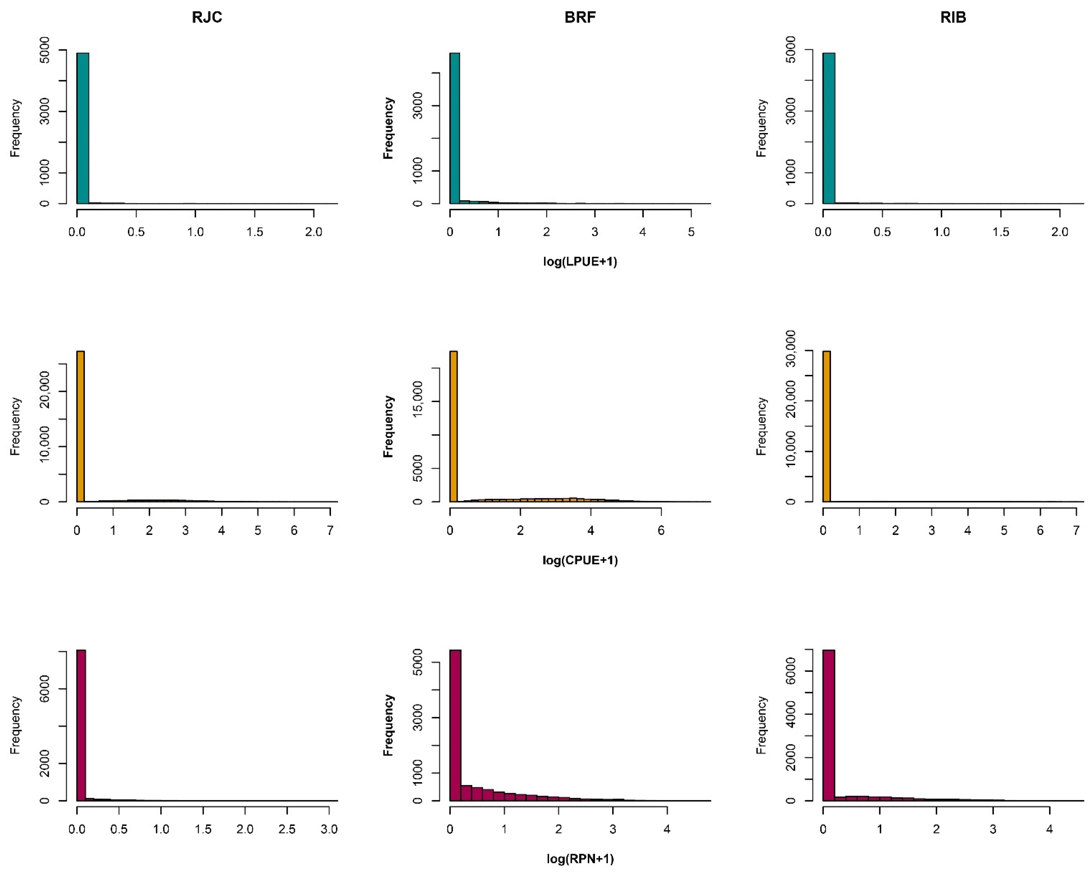
3.1. Nominal Catch Data

Catch distributions were found to be highly skewed, with many zero or low catches, mostly for non-target species, as expected (Figure 1). The LPUE data comprised 4952 landing reports, and such a high proportion of zero catches was observed throughout the studied years for R. clavata, H. dactylopterus, and M. moro at 0.68, 0.62, and 0.88, respectively. For the CPUE database, a total of 31,616 inquiries were analyzed for the three species, with a relative number of zero catches of 0.86 (R. clavata), 0.71 (H. dactylopterus), and 0.94 (M. moro). The data analyzed from the scientific survey accounted for a total of 8618 fishing sets, with a proportion of zeros of 0.92 (R. clavata), 0.59 (H. dactylopterus), and 0.80 (M. moro). The survey database had no information for 1998, 2006, 2009, 2014, and 2015 since the cruise was not executed due to operational issues in those specific years.

3.2. Error–Model Selection (Application)

The Pearson residuals were plotted against the fitted values (Figure S1) as a check of the adequacy of the assumed variance function. The null (expected) pattern of this plot is a distribution of residuals with no trend [16]. The positive–lognormal error distribution was the best model where there was no trend for the residuals of the LPUE, CPUE, and RPN data for all species (Figure S1). The lognormal (1 and c), gamma (1 and c), tweedie, and positive–gamma models showed discrepancies with residuals concentrated at specific plot regions or a few points far from the rest, which indicated the variance function was not appropriate. A positive trend (slope > 0) implies that the assumed variance function is rising too slowly concerning the mean, whereas a negative trend (slope < 0) implies the opposite [16]. Therefore, these error distributions would either underestimate or overstate catch rates for the observed CPUE, LPUE, and RPN.
Diagnostic plots of standardized deviance residuals against the estimated linear predictor are shown in Figure S2. The null pattern is the distribution of the residuals with a mean of zero (dashed line) and a constant range [16]. For all three databases, the gamma (1 and c) and lognormal (1 and c) error distributions showed declining trends in the mean, and the tweedie model showed a systematic change in range with the linear predictor. Curvature can be caused by a variety of factors, including incorrect link function selection, incorrect scale selection for one or more covariates, or the absence of a quadratic component in a covariate [16]. The positive–gamma and positive–lognormal models were consistent with the expected pattern of a mean close to zero.
The link function selected for each error distribution was checked through the plot of the dependent variable (LPUE, CPUE, or RPN) against the linear predictor (Figure S3). The null pattern is a straight line [16], which was observed for all species, databases, and error distributions (Figure S3). This means that the link function was properly chosen for the error distributions analyzed.
To summarize, the model diagnostic plots indicated that the positive–lognormal model was the most appropriate error distribution for fitting the LPUE, CPUE, and RPN data for R. clavata, H. dactylopterus, and M. moro. Consequently, the hurdle–lognormal model was selected as the most suitable error distribution for standardizing such fishery-dependent and independent data for target and non-target species.

3.3. Standardization Procedure

Deviance tables produced from the models and used for selecting relevant explanatory factors and interactions that better explained the data variability for LPUE, CPUE, and RPN data are shown in Tables S1–S3, respectively. The interactions that included the year factor were treated as random interactions, and the final best-fitted model was selected according to the lowest log-likelihood, AIC, and BIC values of binomial and positive–lognormal models of each species (Table S4).
Diagnostic plots of each final model selected from the positive–lognormal error distribution (Figure S4) displayed no strong indication of departure from the null pattern, suggesting that the model selected was well fitted. Subsequently, the standardization procedure was performed using the hurdle–lognormal method (Figure 2). Nominal and standardized abundance indices estimated per year for each species and database are shown in Table S5.

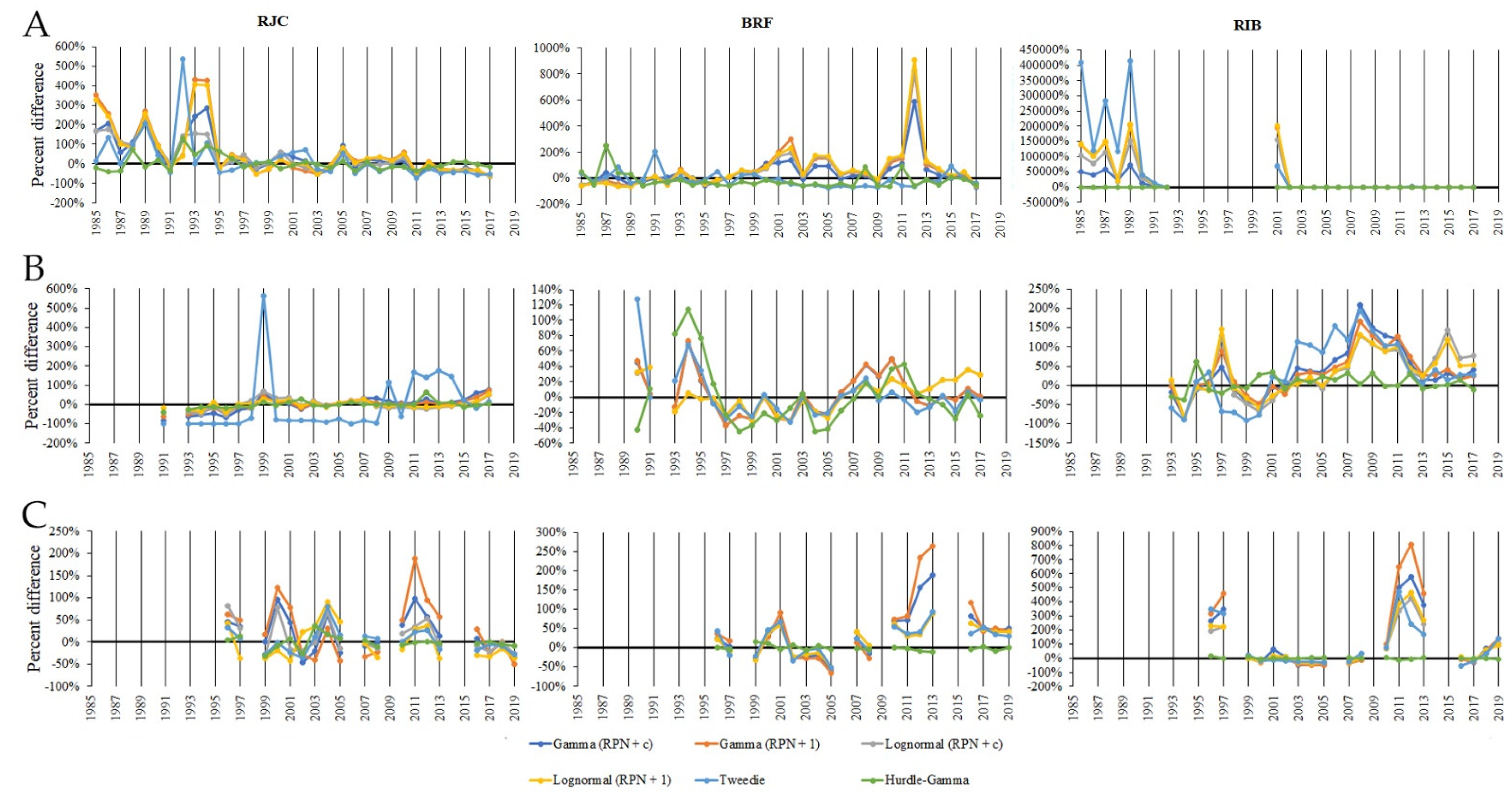
3.4. Consequences of Choosing a Wrong Error–Model

When knowledge of the true status of each species is unknown, an alternative approach for assessing the implications of basing standardization on the incorrect error distribution, in terms of the magnitude of error in the standardized catch rates, is to assume that the results from the selected model provide the most accurate representation of true stock status [21]. Therefore, although the hurdle–lognormal was selected as the best model for standardizing catch rates of all species and databases analyzed, the other explored error distributions were processed with the same method for the model selection, the best model formulation (Table S6), and the diagnostic plots (Figure S5). Standardized catch rates (Table S7) were then summarized as the percent difference from the hurdle–lognormal model.
For the LPUE database (Figure 3), the hurdle–gamma model showed lower percentage differences from the chosen error distribution for the R. clavata and M. moro, with respective average differences of 6% and −7%, while for the H. dactylopterus, the tweedie model showed the lowest ones (−9% on average). The other error–models for R. clavata showed greater discrepancies from the hurdle–lognormal, varying from 23% (tweedie) to 59% (gamma + 1) on average. For H. dactylopterus, the average percentage differences from those from the hurdle–lognormal model varied from −14% (hurdle–gamma) to 70% (lognormal + 1). In the case of M. moro, these average differences in magnitude were greater than 130 times.
The results of the RPN estimates from the hurdle–gamma models were very similar to those from the hurdle–lognormal for all species, with average differences ranging from −1% (R. clavata and H. dactylopterus) to 0% (M. moro; Figure 3). The other error–models for R. clavata showed percentage differences varying from −2% (lognormal + 1) to 28% (gamma + 1) on average. For H. dactylopterus, the RPN estimates from the other models were similar in trend among them but different in magnitude from those from the hurdle–lognormal, with average percentage differences ranging from 22% (tweedie) to 47% (gamma + 1). For M. moro, these percentage differences were greater than 80%.

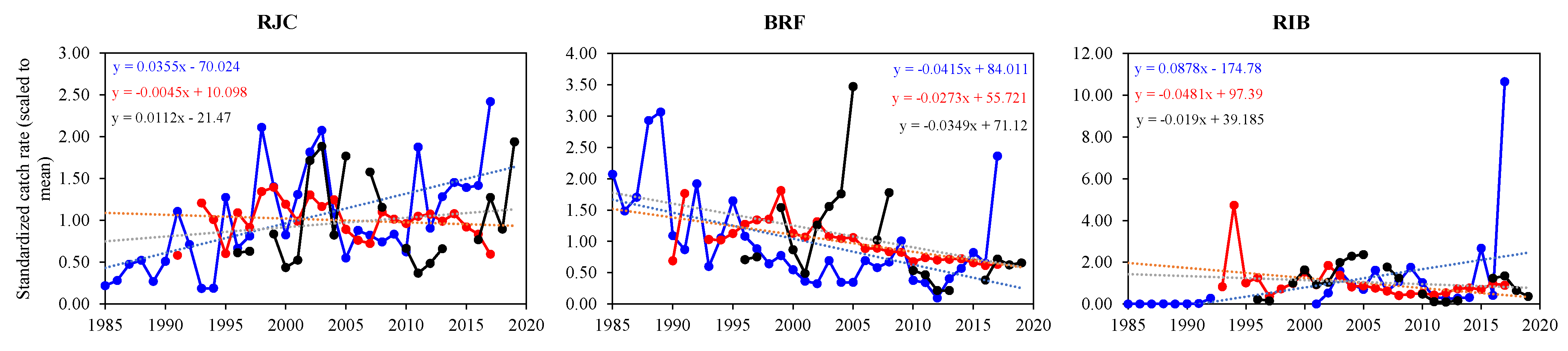
3.5. Catch Trend Comparison between Datasets

Standardized catch rates over the studied years showed varying trends according to each species and across different databases (Figure 2). For R. clavata, both the LPUE and RPN demonstrated an increasing trend (Figure 2), with no significant differences between their intercepts and slopes (Table 2). These trends, in turn, were significantly different from that of the CPUE (Table 2), which was greater in magnitude (intercept) but showed a decreasing tendency (Figure 2). For H. dactylopterus, LPUE, CPUE and RPN were decreasing in trend (Figure 2), with no significant difference between their intercepts and slopes (Table 2). Trend analysis for M. moro indicated significant differences between the intercepts and slopes from the CPUE and RPN compared to that from the LPUE (Table 2), which was lower in magnitude and showed a positive rate of change (i.e., an increasing trend; Figure 2).

3.6. Final Considerations

This study updated and expanded the protocol developed by Ortiz and Arocha [21] for comparing error distribution models to standardize catch rates, aiming to select the best error–model and evaluate model assumptions given the data set characteristics. The use of generalized linear mixed models, particularly the hurdle–lognormal model, resulted in more agreement between model assumptions and observed catch rates. The results confirmed the previously reported consistency of these models with zero-inflated data sets [20,21,48], the importance of model checking and validation procedures for the standardization of nominal catch rates, and the implications of basing the standardization on the incorrect error distribution model [21].
The analyses of catch rates from fishery-dependent and independent data indicated that a few past or recent years could be responsible for the observed differences in the species’ catch trends. For R. clavata, the standardized CPUE values observed in the last three years (2015–2017) were the main responsible for pulling the trend down. This species is primarily found in shallower waters (down to 250 m) around the islands [33,49] and those lower CPUE values are assumed to be related to the observed reduction in both the catches of the species [30] and the fishing effort (days at sea) of the Azorean fleet in coastal areas during the last few years [50] due to the fishing area restrictions [30]. At the same time, as catches declined, a rise in LPUE during the 2015–2017 period might suggest that fewer vessels landed this species and that each of these landing occurrences recorded large captures. This could be explained by the fact that the vessels that continue to operate legally with hook-and-line fishing gear in areas where R. clavata is more likely to be found are typically small (less than 12 m in length), with limited storage capacity and autonomy. This was in part confirmed by this study as métier, gear, vessel size and area, and the interaction between the last three factors and year were significant explanatory variables when modeling catch rates.
For H. dactylopterus, the LPUE, CPUE and RPN were similar in trends. The Azorean spring bottom longline survey is designed to target demersal species such as H. dactylopterus by using a similar fishing strategy to that of the commercial fleet [10]. Consequently, it was expected that after the standardization process, both the fishery-dependent and independent catch rates of H. dactylopterus would show similar trends. This species is usually caught by vessels operating with hook-and-line gears [29], and the harvested population is mainly found in seamount areas at 350–800 m depth [31]. This was validated by this study, which found that métier, gear, depth, and area were important explanatory factors. Finally, the observed declining trends in abundance indices, combined with the sedentary nature of this species, confirmed the already reported vulnerability of this stock to fishing activity [31,51]. As a result, further assessment analyses and effective management strategies are required to establish a balance between stock exploitation and conservation.
In the case of the M. moro species, the observed variations in catch patterns were due to lower LPUE values until the early 1990s and the greatest one in 2017. The first could be associated with the under-exploited phase of its fishery. It is a deep-water species, mainly found at depths ranging from 300 to 2500 m on the outer continental shelf and slope [50]. The exploitation phase of this resource began in the early 2000s; before that, it was captured as a by-catch of the demersal fishery occurring in depths between 200 and 600 m [50]. With the reorientation of the larger vessels to offshore deep waters due to the implementation of fishing area restrictions, the M. moro came to dominate the bottom longline catches in depths between 600 and 1200 m. This was consistent with the analysis of catch rates in the present study because métier, vessel size, target effect, depth zone, and area were significant explanatory factors. Finally, the highest LPUE value in 2017 can represent an error in nominal data and needs to be further investigated.
The primary objective of standardizing catch rates is to generate a relative abundance index. This index is thought to be proportional to population size (e.g., [1,4,5,13,14]). As a result, the abundance index may be utilized as a basis for management measures (e.g., definition of total allowable catches—TACs) either directly, by analyzing the population trend (i.e., rise, decrease, stability) over time, or indirectly, as an input into stock assessment models (e.g., [1,2,3,4,5,6,7,8,9]). Therefore, the definition of the best suitable statistical GLM technique to standardize catch rates made by the present study constitutes a useful outcome for fisheries research and management. However, it is critical to understand the constraints that current data can impose on model application and to plan for the future by selecting what data should be gathered in the future. For example, one of the most important factors in standardizing catch data from commercial fisheries is where the fish were caught. This was evident in this study as area was a significant factor in modeling catch rates from scientific surveys for the three studied species. Therefore, regardless of the method used to standardize the catch rate, it will not perform well unless the appropriate explanatory variables are available.

4. Conclusions

The use of the hurdle–lognormal model outperformed other methods in the different data sources and, therefore, it is recommended as an effective method for standardizing catch rates when it is not possible to perform a comparison with other error–models. Further simulation-based analyses are advised to explore, for example, the effect of other potential sources of bias in the estimation of abundance indices (e.g., fishing area; market demand expressed as reference price, i.e., price per kg; oceanographic factors, e.g., oceanic and atmospheric phenomena, etc.) or the use of clustering-based area stratification for catch and effort data (e.g., [52]). Furthermore, while GLMs are the most commonly used models in fisheries stock assessment and abundance standardization, there have also been analyses that demonstrate the efficacy of using generalized additive models (GAMs; [53]) and, therefore, they should be explored in future studies.

Supplementary Materials

The following supporting information can be downloaded at: https://0-www-mdpi-com.brum.beds.ac.uk/article/10.3390/modelling3010001/s1, Figure S1. Diagnostic plot to detect the adequacy of the assumed variance function in generalized linear models: Pearson residuals plotted versus fitted values for thornback ray Raja clavata (RJC), blackbelly rosefish Helicolenus dactylopterus (BRF), and common mora Mora moro (RIB). The null pattern is a no trend in the residuals. The red line is the loess smoother through the plotted values. A: LPUE (kg landing−1 vessel−1); B: CPUE (kg days at sea−1 vessel−1); C: RPN (ind. 10−3 hooks). Figure S2. Diagnostic plot to check the assumed error distribution in generalized linear models: standardized deviance residuals plotted versus the estimated linear predictor ( η ^ ) for thornback ray Raja clavata (RJC), blackbelly rosefish Helicolenus dactylopterus (BRF), and common mora Mora moro (RIB). The null pattern is a distribution of residuals with mean zero and constant variance. The red line is the loess smoother through the plotted values. A: LPUE (kg landing−1 vessel−1); B: CPUE (kg days at sea−1 vessel−1); C: RPN (ind. 10−3 hooks). Figure S3. Diagnostic plot to check the link function selection in generalized linear models: dependent variable plotted versus the estimated linear predictor ( η ^ ) for thornback ray Raja clavata (RJC), blackbelly rosefish Helicolenus dactylopterus (BRF), and common mora Mora moro (RIB). The null pattern is a straight line. The red line is the loess smoother through the plotted values. A: LPUE (kg landing−1 vessel−1); B: CPUE (kg days at sea−1 vessel−1); C: RPN (ind. 10−3 hooks). Figure S4. Diagnostic plots for positive catch rates of thornback ray Raja clavata (RJC), blackbelly rosefish Helicolenus dactylopterus (BRF), and common mora Mora moro (RIB) to check (I) the adequacy of the assumed variance function, (II) the assumed error distribution, and (III) the link function selection in the best selected models. The null pattern is a no trend in the residuals (I), a distribution of residuals with mean zero and constant variance (II), and a straight line (III). The red line is the loess smoother through the plotted values. A: LPUE (kg landing−1 vessel−1); B: CPUE (kg days at sea−1 vessel−1); C: RPN (ind. 10−3 hooks). Figure S5. Diagnostic plots for positive catch rates of thornback ray Raja clavata (RJC), blackbelly rosefish Helicolenus dactylopterus (BRF), and common mora Mora moro (RIB) to check (I) the adequacy of the assumed variance function, (II) the assumed error distribution, and (III) the link function selection in the best selected models. Results are shown for the other error distributions evaluated. The null pattern is a no trend in the residuals (I), a distribution of residuals with mean zero and constant variance (II), and a straight line (III). The red line is the loess smoother through the plotted values. A: LPUE (kg landing−1 vessel−1); B: CPUE (kg days at sea−1 vessel−1); C: RPN (ind. 10−3 hooks). Table S1. Deviance analysis table of explanatory variables for GLM formulations for thornback ray Raja clavate (RJC), blackbelly rosefish Helicolenus dactylopterus (BRF), and common mora Mora moro (RIB) catch rates (LPUE; kg landing−1 vessel−1) from the Azorean commercial fishery. Significative (P < 0.05) factors and interaction that accounted for 5% or more of the variability are in bold. Table S2. Deviance analysis table of explanatory variables for GLM formulations for thornback ray Raja clavate (RJC), blackbelly rosefish Helicolenus dactylopterus (BRF), and common mora Mora moro (RIB) catch rates (CPUE; kg days at sea−1 vessel−1) from the Azorean commercial fishery. Significative (P < 0.05) factors and interaction that accounted for 5% or more of the variability are in bold. Table S3. Deviance analysis table of explanatory variables for GLM formulations for thornback ray Raja clavate (RJC), blackbelly rosefish Helicolenus dactylopterus (BRF), and common mora Mora moro (RIB) catch rates (RPN; ind. 10−3 hooks) from the Azorean bottom longline survey. Significative (P < 0.05) factors and interaction that accounted for 5% or more of the variability are in bold. Table S4. Analyses of alternative hurdle–lognormal GLMM formulations for thornback ray Raja clavata (RJC), blackbelly rosefish Helicolenus dactylopterus (BRF), and common mora Mora moro (RIB) catch rates (LPUE, CPUE and RPN). Likelihood ratio tests the difference of –2 Restricted Maximum log likelihood (–2 REML) between two nested models. AIC: Akaike’s information criterion; BIC: Bayesian information criterion; LRT: Likelihood ratio test. Table S5. Nominal and standardized LPUE (kg landing−1 vessel−1), CPUE (kg days at sea−1 vessel−1) and RPN (ind. 10−3 hooks) estimates for thornback ray Raja clavata (RJC), blackbelly rosefish Helicolenus dactylopterus (BRF), and common mora Mora moro (RIB) in the Azorean region. LCI and UCI indicate estimated 95% confidence limits. Standardization process was based on the best error distribution. The values are scaled to mean. Table S6. Analyses of alternative GLMM formulations (A: gamma, B: lognormal, C: tweedie, and D: hurdle–gamma) for thornback ray Raja clavata (RJC), blackbelly rosefish Helicolenus dactylopterus (BRF), and common mora Mora moro (RIB). Likelihood ratio tests the difference of –2 REM log likelihood between two nested models. Results are shown for the other error distributions evaluated. AIC: Akaike’s information criterion; BIC: Bayesian information criterion; LRT: Likelihood ratio test. Table S7. Nominal and standardized LPUE (kg landing−1 vessel−1), CPUE (kg days at sea−1 vessel−1), and RPN (ind. 10−3 hooks) estimates for thornback ray Raja clavata (RJC), blackbelly rosefish Helicolenus dactylopterus (BRF) and common mora Mora moro (RIB) in the Azorean region. Results are shown for the others error distributions evaluated (A: gamma, B: lognormal, C: tweedie, and D: hurdle–gamma). The values are scaled to mean.

Author Contributions

R.S. wrote the manuscript with support from O.C., A.N.-P., W.M.-L. and M.P., R.S. and O.C. designed and performed the analysis and interpretation of data. A.N.-P., W.M.-L. and M.P. helped conceive the manuscript. R.S. conceived the original idea and supervised the project. All authors have read and agreed to the published version of the manuscript.

Funding

This work is part of the PESCAz project (ref. MAR-01.03.02-FEAMP-0039) financed by the European Maritime and Fisheries Fund (EMFF) through the Regional Government of the Azores under the MAR2020 operational program. Surveys were funded by the Regional Government of the Azores under the DEMERSAIS project. A.N.-P. was funded by an FCT Ph.D. fellowship (ref. SFRH/BD/124720/2016).

Institutional Review Board Statement

No ethical approval was required from the Portuguese official veterinary department, and this study was performed in accordance with relevant institutional and national guidelines and regulations.

Informed Consent Statement

Not applicable.

Data Availability Statement

The data underlying this article will be shared upon reasonable request to the corresponding author.

Acknowledgments

The authors thank all who participated in field surveys and sample processing onboard the R/V “Arquipélago”.

Conflicts of Interest

The authors declare no conflict of interest.

References

  1. Hilborn, R.; Walters, C.J. Quantitative Fisheries Stock Assessment: Choice, Dynamics and Uncertainty; Springer Science & Business Media: Berlin/Heidelberg, Germany, 2013; ISBN 9781461535980. [Google Scholar]
  2. ICES Guide to ICES advisory framework and principles. Rep. ICES Advis. Comm. 2020, 1–8. [CrossRef]
  3. Cadrin, S.X.; Dickey-Collas, M. Stock assessment methods for sustainable fisheries. ICES J. Mar. Sci. 2015, 72, 1–6. [Google Scholar] [CrossRef] [Green Version]
  4. Cadima, E.L. Fish Stock Assessment Manual; FAO Fisher; FAO: Rome, Italy, 2003; ISBN 9251045054. [Google Scholar]
  5. Sparre, P.; Venema, S.C. Introduction to Tropical Fish Stock Assessment. Part 1 Manual. Part 2 Exercises; FAO: Rome, Italy, 1998; pp. 1–423. [Google Scholar]
  6. Gulland, J.A. Fish population analysis. In Manual of Methods for Fish Stock Assessment; FAO: Rome, Italy, 1969; Volume 4. [Google Scholar]
  7. Quinn, T.J., II; Hoag, S.H.; Southward, G.M. Comparison of two methods of combining catch-per-unit-effort data from geographic regions. Can. J. Fish. Aquat. Sci. 1982, 39, 837–846. [Google Scholar] [CrossRef]
  8. Maunder, M.N.; Punt, A.E. Standardizing catch and effort data: A review of recent approaches. Fish. Res. 2004, 70, 141–159. [Google Scholar] [CrossRef]
  9. Campbell, R.A. CPUE standardisation and the construction of indices of stock abundance in a spatially varying fishery using general linear models. Fish. Res. 2004, 70, 209–227. [Google Scholar] [CrossRef]
  10. Pinho, M.; Medeiros-Leal, W.; Sigler, M.; Santos, R.; Novoa-Pabon, A.; Menezes, G.; Silva, H. Azorean demersal longline survey abundance estimates: Procedures and variability. Reg. Stud. Mar. Sci. 2020, 39, 101443. [Google Scholar] [CrossRef]
  11. Garrod, D.J. Effective fishing effort and the catchability coefficient q. Rapport et process verbaux des réunions du Conseil International pour l’Exploration de la Mer 1964, 155, 66–70. [Google Scholar]
  12. Bishop, J. Standardizing fishery-dependent catch and effort data in complex fisheries with technology change. Rev. Fish Biol. Fish. 2006, 16, 21–38. [Google Scholar] [CrossRef]
  13. Ye, Y.; Dennis, D. How reliable are the abundance indices derived from commercial catch—Effort standardization? Can. J. Fish. Aquat. Sci. 2009, 66, 1169–1178. [Google Scholar] [CrossRef]
  14. Maunder, M.N. A general framework for integrating the standardization of catch per unit of effort into stock assessment models. Can. J. Fish. Aquat. Sci. 2001, 58, 795–803. [Google Scholar] [CrossRef]
  15. Nelder, J.A.; Wedderburn, R.W.M. Generalized linear models. J. R. Stat. Soc. Ser. A 1972, 135, 370–384. [Google Scholar] [CrossRef]
  16. McCullagh, P.; Nelder, J.A. Generalized Linear Models, 2nd ed.; Chapman and Hall: London, UK, 1989. [Google Scholar]
  17. Jorgensen, B. The Theory of Dispersion Models; CRC Press: Boca Rato, FL, USA, 1997. [Google Scholar]
  18. Jorgensen, B. Exponential Dispersion Models. J. R. Stat. Soc. Ser. B 1987, 49, 127–162. [Google Scholar] [CrossRef]
  19. Lo, N.C.; Jacobson, L.D.; Squire, J.L. Indices of Relative Abundance from Fish Spotter Data based on Delta-Lognornial Models. Can. J. Fish. Aquat. Sci. 1992, 49, 2515–2526. [Google Scholar] [CrossRef]
  20. Stefánsson, G. Analysis of groundfish survey abundance data: Combining the GLM and delta approaches. ICES J. Mar. Sci. 1996, 53, 577–588. [Google Scholar] [CrossRef]
  21. Ortiz, M.; Arocha, F. Alternative error distribution models for standardization of catch rates of non-target species from a pelagic longline fishery: Billfish species in the Venezuelan tuna longline fishery. Fish. Res. 2004, 70, 275–297. [Google Scholar] [CrossRef]
  22. Shono, H. Application of the Tweedie distribution to zero-catch data in CPUE analysis. Fish. Res. 2008, 93, 154–162. [Google Scholar] [CrossRef] [Green Version]
  23. Carvalho, F.C.; Murie, D.J.; Hazin, H.G.; Leite-Mourato, B.; Travassos, P.; Burgess, G.H. Catch rates and size composition of blue sharks (Prionace glauca) caught by the Brazilian pelagic longline fleet in the southwestern Atlantic Ocean. Aquat. Living Resour. 2010, 23, 373–385. [Google Scholar] [CrossRef] [Green Version]
  24. Pons, M.; Domingo, A.; Sales, G.; Fiedler, F.N.; Miller, P.; Giffoni, B.; Ortiz, M. Standardization of CPUE of loggerhead sea turtle (Caretta caretta) caught by pelagic longliners in the Southwestern Atlantic Ocean. Aquat. Living Resour. 2010, 23, 65–75. [Google Scholar] [CrossRef]
  25. Thorson, J.T.; Cunningham, C.J.; Jorgensen, E.; Havron, A.; Hulson, P.J.F.; Monnahan, C.C.; von Szalay, P. The surprising sensitivity of index scale to delta-model assumptions: Recommendations for model-based index standardization. Fish. Res. 2021, 233, 105745. [Google Scholar] [CrossRef]
  26. Simpfendorfer, C.A.; Hueter, R.E.; Bergman, U.; Connett, S.M.H. Results of a fishery-independent survey for pelagic sharks in the western North Atlantic, 1977–1994. Fish. Res. 2002, 55, 175–192. [Google Scholar] [CrossRef]
  27. EU Council Regulation (EC) No 199/2008 of 25 February 2008 concerning the establishment of a Community framework for the collection, management and use of data in the fisheries sector and support for scientific advice regarding the Common Fisheries Policy. Off. J. Eur. Union L 2008, 60, 1–12.
  28. Menezes, G.M.; Sigler, M.F.; Silva, H.M.; Pinho, M.R. Structure and zonation of demersal fish assemblages off the Azores Archipelago (mid-Atlantic). Mar. Ecol. Prog. Ser. 2006, 324, 241–260. [Google Scholar] [CrossRef] [Green Version]
  29. Santos, R.V.S.; Silva, W.M.M.L.; Novoa-Pabon, A.M.; Silva, H.M.; Pinho, M.R. Long-term changes in the diversity, abundance and size composition of deep sea demersal teleosts from the Azores assessed through surveys and commercial landings. Aquat. Living Resour. 2019, 32, 25. [Google Scholar] [CrossRef] [Green Version]
  30. Santos, R.; Novoa-Pabon, A.; Silva, H.; Pinho, M. Elasmobranch species richness, fisheries, abundance and size composition in the Azores archipelago (NE Atlantic). Mar. Biol. Res. 2020, 16, 103–116. [Google Scholar] [CrossRef]
  31. Santos, R.; Pabon, A.; Silva, W.; Silva, H.; Pinho, M. Population structure and movement patterns of blackbelly rosefish in the NE Atlantic Ocean (Azores archipelago). Fish. Oceanogr. 2020, 29, 227–237. [Google Scholar] [CrossRef]
  32. Santos, R.; Medeiros-Leal, W.; Pinho, M. Stock assessment prioritization in the Azores: Procedures, current challenges and recommendations. Arquipelago Life Mar. Sci. 2020, 37, 45–64. [Google Scholar]
  33. Santos, R.; Medeiros-Leal, W.; Pinho, M. Synopsis of biological, ecological and fisheries-related information on priority marine species in the Azores region. Arquipelag. Life Mar. Sci. 2020, 1, 1–138. [Google Scholar]
  34. Zuur, A.; Ieno, E.N.; Walker, N.; Saveliev, A.A.; Smith, G.M. Mixed Effects Models and Extensions in Ecology with R; Springer Science & Business Media: New York, NY, USA, 2009; ISBN 978-0-387-98957-0. [Google Scholar]
  35. Zuur, A.F.; Ieno, E.N. Beginner′s Guide to Zero-Inflated Models with R; Highland Statistics Ltd.: Newburgh, UK, 2016; ISBN 978-0-9571741-8-4. [Google Scholar]
  36. Ortiz, M.; Legault, C.M.; Ehrhardt, N.M. An alternative method for estimating bycatch from the U.S. shrimp trawl fi shery in the Gulf of Mexico, 1972–1995. Fish. Bull. 2000, 98, 583–599. [Google Scholar]
  37. Cooke, J.G. A procedure for using catch-effort indices in bluefin tuna assessments. Collect. Vol. Sci. Pap. ICCAT 1997, 46, 228–232. [Google Scholar]
  38. Pinheiro, J.C.; Bates, D.M. Mixed-Effects Models in S and S-PLUS; Springer: New York, NY, USA, 2000; ISBN 978-0-387-98957-0. [Google Scholar]
  39. Walter, J.; Ortiz, M. Derivation of the delta-lognormal variance estimator and recommendation for approximating variances for two-stage cpue standardization models. Collect. Vol. Sci. Pap. ICCAT 2012, 68, 365–369. [Google Scholar]
  40. Zar, J.H. Biostatistical Analysis, 5th ed.; Prentice-Hall/Pearson: Teaneck, NJ, USA, 2010. [Google Scholar]
  41. McDonald, J.H. Handbook of Biological Statistics—Paired t-test. Sparky House Publ. 2014, 180–185. [Google Scholar]
  42. R Core Team R: A Language and Environment for Statistical Computing; R Foundation for Statistical Computing: Vienna, Austria, 2020.
  43. Venables, W.N.; Ripley, B.D. Modern Applied Statistics with S, 4th ed.; Springer: New York, NY, USA, 2002. [Google Scholar]
  44. Sarkar, D. Lattice: Multivariate Data Visualization with R; Springer: New York, NY, USA, 2008. [Google Scholar]
  45. Lenth, R. V Least-Squares Means: The R Package lsmeans. J. Stat. Softw. 2016, 69, 1–33. [Google Scholar] [CrossRef] [Green Version]
  46. Bates, D.; Mächler, M.; Bolker, B.; Walker, S. Fitting Linear Mixed-Effects Models Using lme4. J. Stat. Softw. 2015, 67, 1–48. [Google Scholar] [CrossRef]
  47. Dunn, P.K. Tweedie: Evaluation of Tweedie Exponential Family Models, R package version 2.3; 2017. [Google Scholar]
  48. Pennington, M. Estimating the mean and variance from highly skewed marine data. Fish. Bull. 1996, 94, 498–505. [Google Scholar]
  49. Santos, R.; Medeiros-Leal, W.; Novoa-Pabon, A.; Crespo, O.; Pinho, M. Biological Knowledge of Thornback Ray (Raja clavata) from the Azores: Improving Scientific Information for the Effectiveness of Species-Specific Management Measures. Biology 2021, 10, 676. [Google Scholar] [CrossRef]
  50. Santos, R.; Medeiros-Leal, W.; Crespo, O.; Novoa-Pabon, A.; Pinho, M. Contributions to Management Strategies in the NE Atlantic Regarding the Life History and Population Structure of a Key Deep-Sea Fish (Mora moro). Biology 2021, 10, 522. [Google Scholar] [CrossRef]
  51. Santos, R.; Medeiros-Leal, W.; Novoa-Pabon, A.; Silva, H.; Pinho, M. Demersal fish assemblages on seamounts exploited by fishing in the Azores (NE Atlantic). J. Appl. Ichthyol. 2021, 37, 198–215. [Google Scholar] [CrossRef]
  52. Ono, K.; Punt, A.E.; Hilborn, R. Think outside the grids: An objective approach to define spatial strata for catch and effort analysis. Fish. Res. 2015, 170, 89–101. [Google Scholar] [CrossRef]
  53. Potts, S.E.; Rose, K.A. Evaluation of GLM and GAM for estimating population indices from fishery independent surveys. Fish. Res. 2018, 208, 167–178. [Google Scholar] [CrossRef]
Figure 1. Frequency distribution of nominal LPUE (kg landing−1 vessel−1), CPUE (kg days at sea−1 vessel−1), and RPN (ind. 10−3 hooks) data for thornback ray Raja clavata (RJC), blackbelly rosefish Helicolenus dactylopterus (BRF), and common mora Mora moro (RIB) in the Azorean region.
Modelling 03 00001 g001
Figure 2. Standardized LPUE (in blue), CPUE (in red), and RPN (in black color) for thornback ray Raja clavata (RJC), blackbelly rosefish Helicolenus dactylopterus (BRF), and common mora Mora moro (RIB) in the Azorean region. The dashed lines represent the linear regressions (the equations are indicated in the graph).
Modelling 03 00001 g002
Figure 3. Percent differences between annual standardized catch rates of thornback ray Raja clavata (RJC), blackbelly rosefish Helicolenus dactylopterus (BRF), and common mora Mora moro (RIB) based on various error distributions and those from the best one (zero line). (A) LPUE (kg landing−1 vessel−1); (B) CPUE (kg days at sea−1 vessel−1); (C) RPN (ind. 10−3 hooks). The standardized CPUE indices (Figure 3) for R. clavata from the gamma (c and 1), lognormal (c and 1), and hurdle–gamma models were similar, with percentage differences ranging from −1% (hurdle–gamma) to 2% (gamma + c). The estimates from the tweedie error distribution showed greater variations, with an average difference of −6%. For H. dactylopterus, percentage differences from those estimates of standardized CPUE for the hurdle–lognormal model were less than 4% on average. However, these differences could reach about 127% in some years. For the M. moro, the hurdle–gamma model showed the lower percentage difference from the hurdle–lognormal, with an average of 6%. The other error–models had greater discrepancies, ranging from 32% (lognormal + c) to 35% (tweedie and gamma + c).
Modelling 03 00001 g003
Table 1. Explanatory variables (main factors) used in the model formulations for standardized thornback ray Raja clavata, blackbelly rosefish Helicolenus dactylopterus (BRF), and common mora Mora moro catch rates.
Landing ReportsFishing InquiriesScientific Survey
VariableTypeObservationsVariableTypeObservationsVariableTypeObservations
YearCategorical (33)Period: 1985–2017YearCategorical (27)Period: 1990–2017YearCategorical (19)Period: 1996–2019 (except 1998, 2006, 2009, 2014 and 2015)
QuarterCategorical (4)1: January–MarchQuarterCategorical (4)1: January–March
2: April–June2: April–JuneMonthCategorical (5)March
3: July–September3: July–September April
4: October–December4: October–December May
Vessel lengthCategorical (5)1: ≤10 mVessel lengthCategorical (5)1: ≤10 m June
2: >10 and ≤12 m2: >10 and ≤12 m July
3: >12 and ≤18 m3: >12 and ≤18 mMoonCategorical (4)1: New moon
4: >18 and ≤24 m4: >18 and ≤24 m 2: First quarter
5: >24 and ≤40 m5: >24 and ≤40 m 3: Full moon
MétierCategorical (12)HDP: hand pickingGearCategorical (5)LL: Longlines 4: Last quarter
HUN: species removal by huntingHL: HandlinesAreaCategorical (10)AÇO: Açores bank
FPO_CRU: pots and traps for crustaceansNT: Nets PAL: Princess Alice bank
FPO_FIF: pots and traps for fishTP: Traps and pots FPI: Faial and Pico
GNS_FIF: gillnets for coastal demersal and pelagic fishMG: Multigear GRA: Graciosa
LHP_CEP: handlines for cephalopods—squidsDepth (mean depth of fishing operation)Categorical (3)1: Shallow (<200 m) SJO: São Jorge
LHP_FIF: handlines for demersal fish2: Intermediate (200–600 m) TER: Terceira
LHP_MDP: handlines locally called “corrico” for pelagic fish3: Deep (>600 m) SMA: Santa Maria
LHP_LPF (pole and lines for pelagic fish)Target effect (percentage of species-specific catch related to the total catch)Categorical (4)1: 1st quartile (≤25%) SMI: São Miguel
LLD: drifting longlines for pelagic and demersal fish2: 2nd quartile (>25% and ≤50%) MPR: Mar da Prata bank
LLS_DEF: set longlines for pelagic and demersal fish3: 3rd quartile (>50% and ≤75%) FCO: Flores and Corvo
PS_SPF: purse seines for small pelagic fish4: 4th quartile (>75%)DepthCategorical (24)from 0 to 1200 m by 50 m intervals (1: 0–50 m, 2: 50–100 m, …, 24: 1150–1200 m)
Target effect (percentage of species-specific catch related to the total catch)Categorical (4)1: 1st quartile (≤ 25%)
2: 2nd quartile (> 25% and ≤ 50%) Soak time (time during which the hooks were in the water)Categorical (8)Time expressed in hours from 2 to 8 by 1 h intervals (2: ≥1.5 and <2.5, 3: ≥2.5 and <3.5, …, 8: ≥7.5 and <8.5)
3: 3rd quartile (> 50% and ≤ 75%)
4: 4th quartile (> 75%)
Table 2. Results of analysis of covariance (ANCOVA) for differences between regression lines from annual standardized LPUE (kg landing−1 vessel−1), CPUE (kg days at sea−1 vessel−1), and RPN (ind. 10−3 hooks) catch rates by species (RJC: thornback ray Raja clavata, BRF: blackbelly rosefish Helicolenus dactylopterus, RIB: common mora Mora moro). Significant differences at the 0.05 significance level are in bold.
RJCBRFRIB
EstimateStd. ErrortpEstimateStd. ErrortpEstimateStd. Errortp
Intercept
LPUE−70.02415.933−4.395<0.00184.01121.0193.997<0.001−174.77750.969−3.4290.001
CPUE80.12227.6752.8950.005−28.29035.019−0.8080.422272.16789.8863.0280.004
RPN48.55432.4601.4960.139−12.89142.821−0.3010.764213.962100.3562.1320.037
Slope
LPUE0.0350.0084.458<0.001−0.0410.011−3.949<0.0010.0880.0253.4490.001
CPUE−0.0400.014−2.8980.0050.0140.0170.8110.420−0.1360.045−3.0290.004
RPN−0.0240.016−1.5020.1380.0070.0210.3070.760−0.1070.050−2.1350.037
Publisher’s Note: MDPI stays neutral with regard to jurisdictional claims in published maps and institutional affiliations.

