Thickness and Color Structure of Center Vortices in Gluonic SU(2) QCD


Atominstitut, Technische Universität Wien, 1020 Wien, Austria
*
Author to whom correspondence should be addressed.
Particles 2020, 3(2), 444-455; https://0-doi-org.brum.beds.ac.uk/10.3390/particles3020031
Submission received: 30 April 2020
/
Revised: 19 May 2020
/
Accepted: 21 May 2020
/
Published: 22 May 2020
Abstract
:In search for an effective model of quark confinement we study the vacuum of SU(2) quantum chromodynamic with lattice simulations using Wilson action. Assuming that center vortices are the relevant excitations causing confinement, we analyzed their physical size and their color structure. We present confirmations for a vanishing thickness of center vortices in the continuum limit and hints at their color structure. This is the first time that algorithms for the detection of thick center vortices based on non-trivial center regions has been used.
PACS:
11.15.Ha; 12.38.Gc1. Introduction
The strong interaction relevant for quantum chromodynamic is governed by an SU(3) symmetric Lagrangian. One of the most important non-perturbative properties of QCD is confinement. It results from a non-perturbative vacuum. This raises the question about the corresponding non-perturbative degrees of freedom. The center vortex model [1,2] is based on the idea that the important ingredients are center degrees of freedom in the form of closed magnetic flux tubes, quantised to the two non-trivial center elements of SU(3). In this first study of the detection of finite center regions, we are investigating SU(2)-QCD which is also confining and breaks chiral symmetry dynamically [3]. It has only one non-trivial center element and one species of magnetic flux tubes. Working with the Wilson action, the lattice spacing is adjusted by choosing the inverse coupling , which is related to the coupling constant g by . In this type of studies the closed color magnetic flux lines percolating the vacuum, are located by P-vortices [4], identified in the direct maximal center gauge, which aims at finding gauge matrices so that
with , an element of SU(2), being the gluonic link variable at lattice point x in direction . We chose the gauge by a modified simulated annealing procedure preserving non-trivial center regions, regions whose perimeter evaluates to a non-trivial center element. This is done by rejecting transformations that after center projection would result in the vanishing of non-trivial center regions [5]. The details are described in ref. [6]. As long as non-trivial center regions vanish we keep the simulated annealing temperature high.
Plaquettes pierced by a P-vortex are found by projection onto the central degrees of freedom, in SU(2) just a sign,
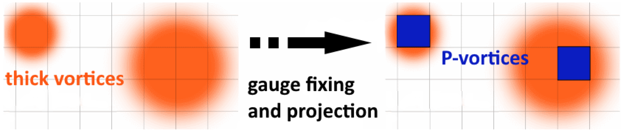
They evaluate to the non-trivial center element in the projected configuration. The vortex detection can be seen as a best fit procedure of a thin vortex configuration to a given field configuration [4,7], see Figure 1: gauge dependent P-vortices of singular thickness locate gauge independent thick vortices of finite thickness [8].
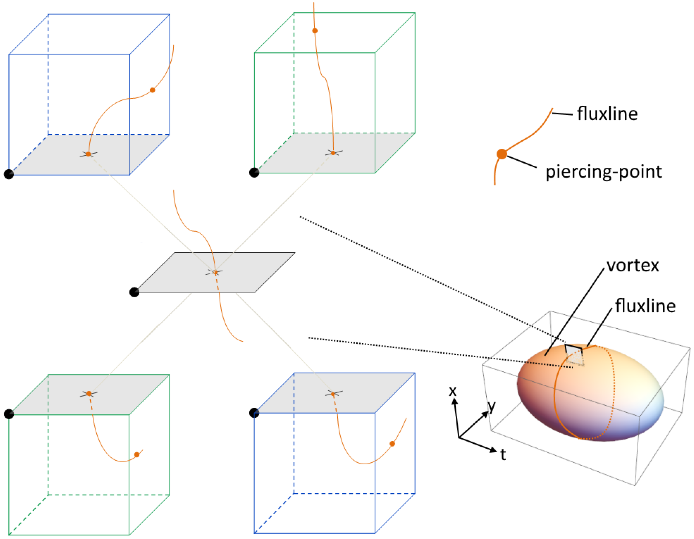
Center projection leads to plaquettes with non-trivial center values. The P-plaquettes form P-vortices, closed surfaces in dual space; see Figure 2. We relate the thickness of the vortex to the area A of the cross section by .
Assuming independence of vortex piercings, the vortex density , the number of P-plaquettes per unit volume, is related to the string tension by
Correlations of such piercings lead to an overestimation of . To reduce the amount of such short range fluctuations, smoothing procedures of the vortex surface are used [9]. A determination of , more independent from short range fluctuations is given using Wilson loops by the Creuz ratios
Comparing the Creutz ratios we can assure that the center projected configuration and the full configuration have the same lattice spacing and that the center projection captures the full string tension. The lattice spacing is defined via the physical value of the string tension and calculates the string tension in lattice units, , to
For the first time we present results based on our algorithms for locating thick vortices. We get indications for a vanishing thickness of center vortices in the continuum limit, which is compatible with the findings in [10]. In addition, we found hints of a color structure on the vortex surface.
2. Materials and Methods
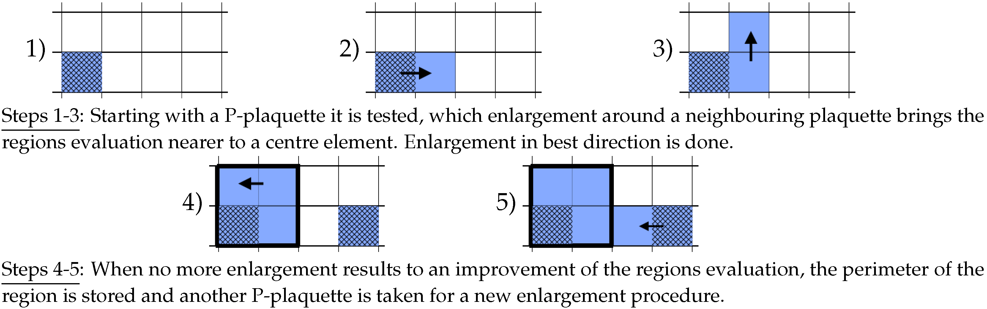
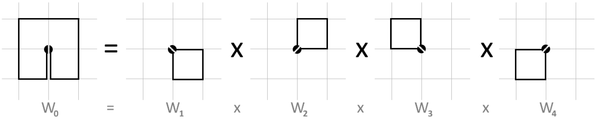
After gauge fixing to direct maximal center gauge preserving non-trivial center regions during simulated annealing with up to 2700 steps, we identify P-plaquettes in the . We check how good we capture the confining excitations by calculating the Creutz ratios. Our algorithm detects non-trivial center regions by the identification of loops enclosing thick vortices in the : starting with the full plaquette matrices at the position of the identified P-plaquettes, the loop forming the plaquette is enlarged by pushing its perimeter outwards over neighboring plaquettes so that the path integrated product of the enlarged region gets closer to the non trivial center element; see Figure 3.
When all minimal planar loops are identified that enclose the thick vortex, its thickness can be estimated by counting the number of enclosed plaquettes. We take care of the scaling of the lattice spacing a and fit the cross section of the piercing by
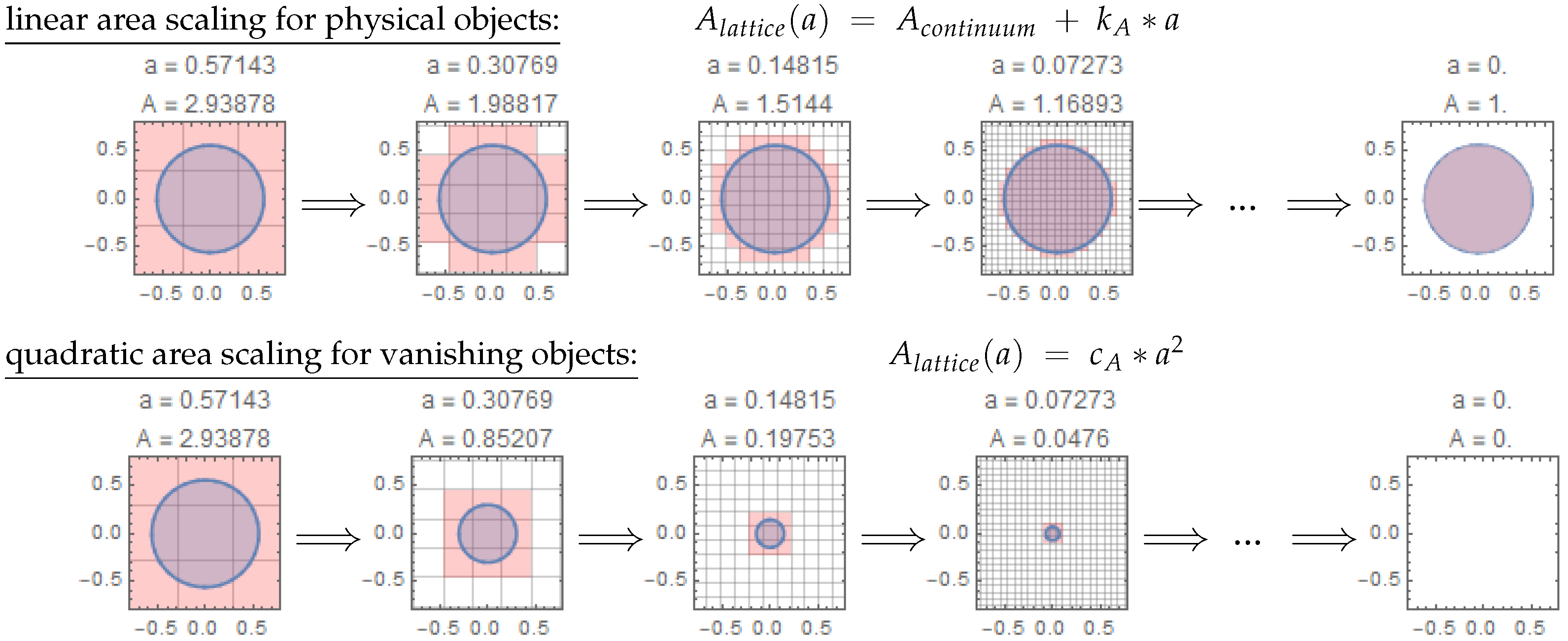
with fit-parameters k and c. With the diagrams in the lower row of Figure 4, we want to show that the term quadratic in a detects whether cross sections have contributions proportional to the plaquette area. The term proportional a results from the finite resolution of the boundary; see the upper row of Figure 4. The constant term indicates the predicted size of the physical area in the continuum limit.
To study the color structure of the vacuum, a quantity measuring the homogeneity of the flux building up the vortex is needed. The concept was first presented in [11] and consists of referencing different plaquettes to the same lattice point; see Figure 5.
By factorizing the plaquettes into Pauli matrices ,
we define the S2-homogeneity of m plaquettes referenced to the same lattice point using the vectors as
In this work we will only compare two plaquettes for calculating ( in Equation (8)) because this allows to clearly distinguish different properties as is shown in the next section. We assume a scaling dependency with the lattice spacing a of the form
and fit , and to the data taken from the lattice. The value of corresponds to the continuum limit of the color homogeneity. The S2-homogeneity of plaquettes at position x and with can be related to the difference
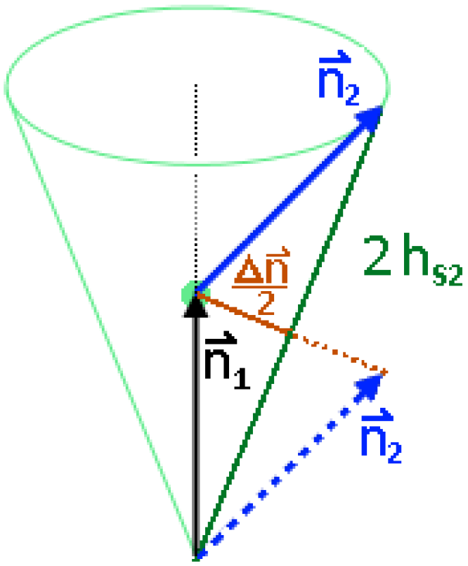
With given color vector , the second vector is only fixed to the cone shown in Figure 6.
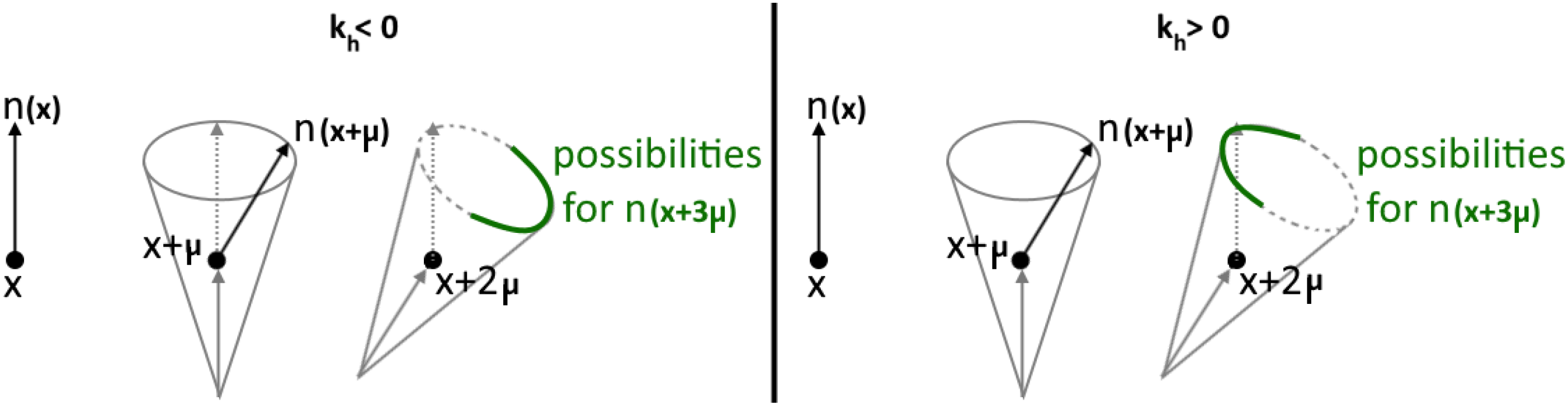
The sign of k indicates whether we have long or short ranged fluctuations.
Negative k indicates, that the increases with growing distance between the considered color vectors and positive implies decreasing with growing distance; see Figure 7.
For an analysis of a geometric structure we need to define some terms, distinguishing different orientations and positions of pairs of plaquettes in spacetime. By calculating the S2-homogeneity of two neighboring plaquettes in the same plane in spacetime we can distinguish four “planar” color homogeneities:
- Inside the thick vortex (“Interior”): both plaquettes lying within the loop;
- Outside the thick vortex (“Outside”): both plaquettes lying outside the loop;
- On the vortex edge (“Edge”): one plaquette within and one outside the thick vortex;
- Average over the whole lattice (“Vacuum”): no further criteria.
Two non-planar plaquettes are considered “longitudinal” if they belong to the same cube, see Figure 2 and therefore can be pierced by the same flux line. For two such non-planar plaquettes it is not necessary that they are of same direction and we distinguish four relative positions in order to study the corresponding S2-homogeneities:
- Along the vortex flux (“online”): both plaquettes are P-plaquettes;
- Outside the vortex (“offline”): non of the plaquettes is a P-plaquette;
- Trespassing the vortex (“leaving”): only one of the two plaquettes is a P-plaquette;
- Average over the whole lattice (“Vacuum”): no criteria.
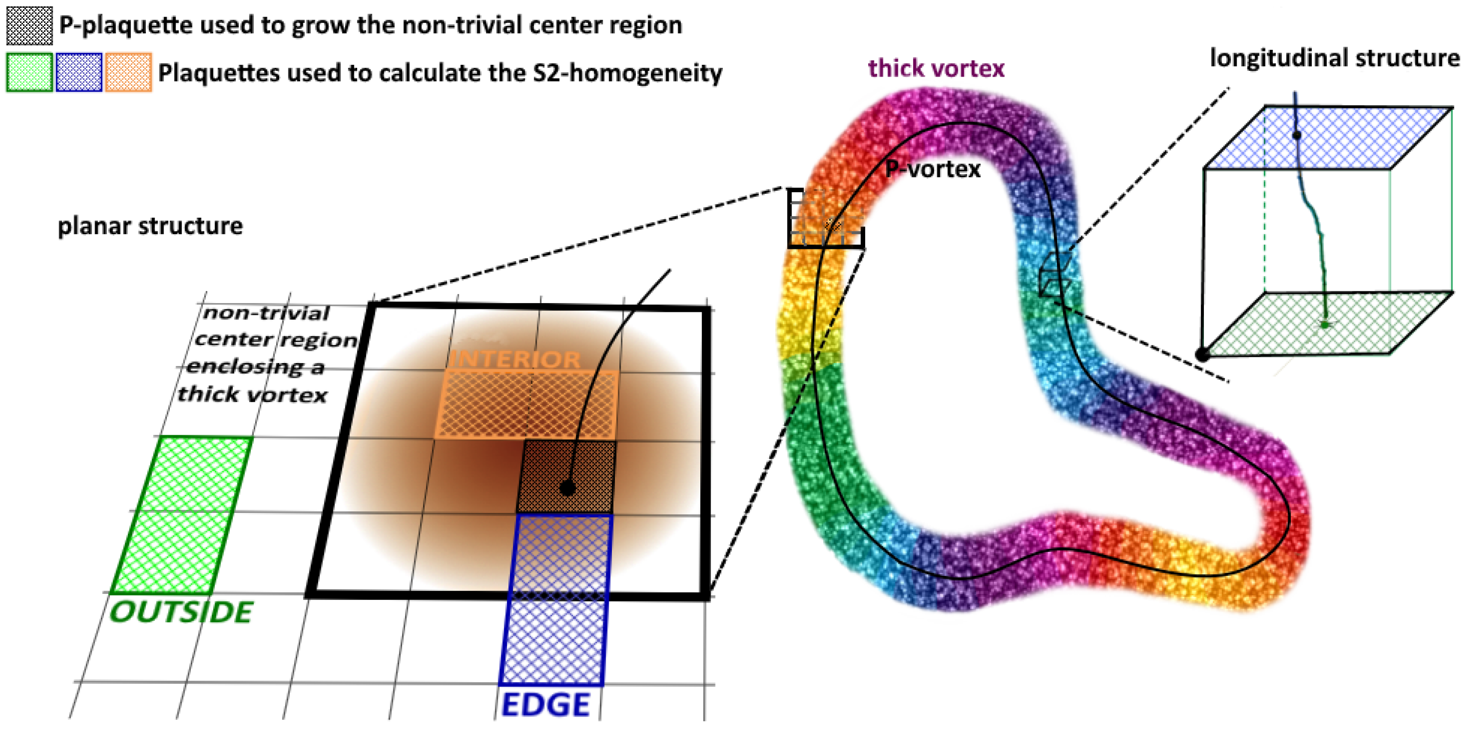
Figure 8 tries to clarify the idea behind these planar and longitudinal properties. The S2-homogeneities of planar and longitudinal vacuum can deviate because the distance of the compared plaquettes is not necessarily identical.
As calculations of the lattice spacing require much more statistics than we need for the calculations of the piercing area and the color structure, we do a cubic interpolation of the literature values given in Table 1 to determine the lattice spacing.
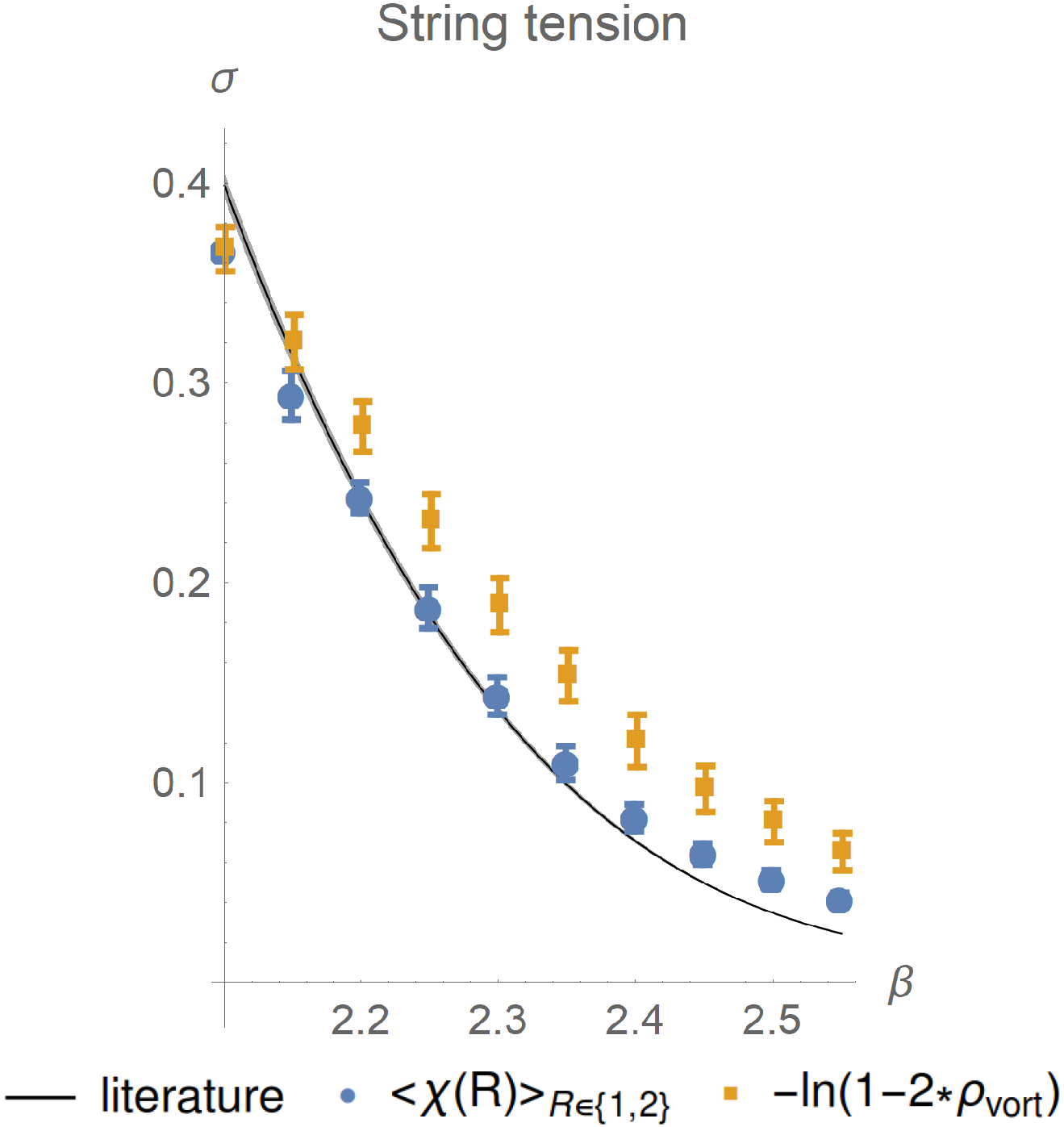
Our calculations cover an interval from to in steps of 0.05. To each value of we generate 120 configurations with Wilson action, respectively, 10 for lattices of size and and 100 for lattices of size . By calculating the string tension via Creutz ratios in the center projected configuration and comparing with the literature values we can quantify how good we detected the center vortices and by approximating the string tension via the vortex density we can check how many short range fluctuations perturb our analysis. As can be seen in Figure 9, our identification of the excitations relevant for confinement are quite satisfactory for the middle -regime, although slightly underestimate the literature values in the lower regime and slightly overestimate it for higher . We accept an overestimated vortex density in order not to overlook excitations relevant for confinement when reconstructing thick vortices.
3. Results
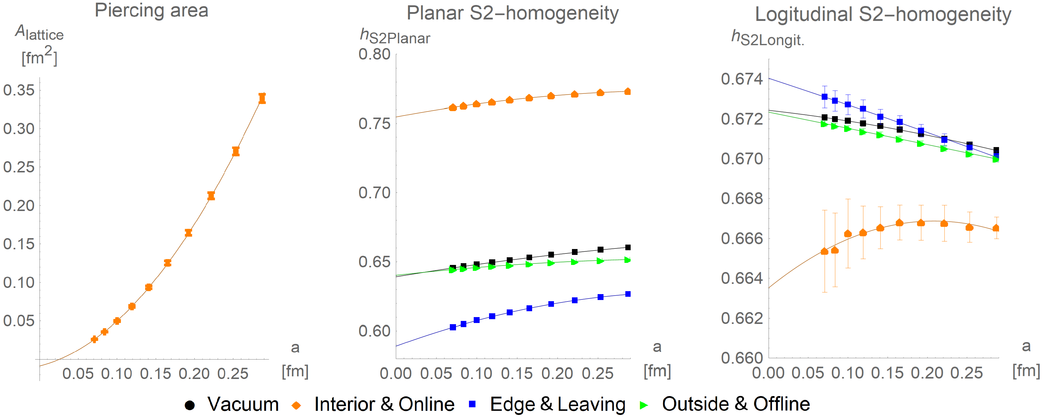
Figure 10 shows our results and fits with extrapolations to the continuum limit. All parameters of the respective fits are shown with full value and standard error in the tables below. The T-statistic and P-value are shown to check the quality of the fit. First we present indications for a vanishing thickness of vortices in the continuum limit, then we discuss their color structure.
In the left part of Figure 10 and in Table 2 the dominance of the quadratic term with factor over the linear factor and the small non-physical negative value of for the piercing area indicate a vanishing vortex thickness in the continuum, remember Figure 4. This is also strengthened by the fact, that within errors we find equal continuum extrapolations of S2-homogeneities for the vacua and outside and offline the vortex, see green and black line corresponding to Outside AND Offline and Vacuum in the middle and right of Figure 10. In the continuum limit the planar homogeneity (middle) of the vacuum of is compatible to the planar homogeneity outside the vortex ; see Table 3. The longitudinal homogeneity (right) of the vacuum of is compatible to the longitudinal homogeneity offline the vortex ; see Table 4. Furthermore, the factors of the linear terms are compatible for the whole vacuum (planar , longitudinal ) and outside/offline the vortex (planar , longitudinal ).
Within errors the quadratic factors for the vacuum (planar and longitudinal ) are identical to those outside/offline the vortex (planar and longitudinal ). This is compatible to the assumption, that the two volumina, that is, whole vacuum and outside/offline the vortex, coincide.
In Table 3 the two positive signs of the and the two small values of the outside the vortex and for the vacuum indicate that there are no long range fluctuations (remember Figure 7) of the color vector, although the high P-values demand caution with this interpretation.
The high planar S2-homogeneity of within the vortex, compared to the vacuum value of (see Table 3 and Table 5) are also in favour of a vanishing vortex thickness; as a singular vortex can not have planar structure, a high planar S2-homogeneity inside the vortex cross section is expected.
The positive value of inside this piercing area indicates that the planar homogeneity of the vortex is disturbed only by short range fluctuations (remember Figure 8) of the color vector, which is again in favor of a non existing planar color structure, hence vanishing thickness of the vortex.
On the vortex edge the planar S2-homogeneity with a value of is below the vacuum; compare Table 6 to Table 3.
The positive value of and the non-vanishing value of at the vortex edge indicate a big difference of the color vector inside and outside of the non-trivial center regions.
The longitudinal measurement depicted on the right side of Figure 10 shows that the color vector fluctuates strongly along the vortex surface. Comparing Table 7 to Table 4, the longitudinal S2-homogeneity of along the vortex is below the vacuum value of . This hints at a non-trivial, longitudinal color structure of the vortex surface. The positive value of along the vortex line (online) indicates long range fluctuations of the color vector, but to exclude a negative value more data has to be collected. Furthermore, the value of along the vortex requires more statistics. A fit up to quadratic order might not be the optimum for the color homogeneity along the vortex, possible is also a linear raise with increasing lattice spacing until saturation is reached. As of that, the error of along the vortex might be underestimated by the fit. Of interest is further, that the longitudinal S2-homogeneity leaving, that is, one plaquette being pierced by the vortex and one not, with a value of is slightly above the homogeneity of the surrounding vacuum, compare Table 8 to Table 4.
The longitudinal S2-homogeneity online is calculated solely on P-plaquettes, but the thick vortex spans over several plaquettes. We know that this measurement oversees neighboring plaquettes that belong to the thick vortex.
4. Discussion
We have presented strong evidence for a vanishing thickness of SU(2) center vortices in the continuum limit and indications for a longitudinal color structure of the vortex surface: along the vortex and when trespassing the vortex surface the fluctuations of the color vectors are stronger than in the surrounding vacuum. Our data favor a model of surface like vortices of thickness vanishing in the continuum limit with non-trivial color structure reflected by the behavior of the longitudinal S2-homogeneity along the flux lines building up the surface. Fluctuations of the color vector covering the whole along the vortex surface could further lead to a topological charge [17,18,19]. When projecting the color vectors to a given axis defined by an abelian subgroup, we get positive and negative regions separated by world lines of magnetic monopoles.
The vanishing vortex thickness in the continuum limit hints at infinitely thin strings populating the vacuum. The corresponding action diverges and has to be canceled by an entropic contribution [10]. The longitudinal color structure relates center vortices to abelian monopoles. For them, corresponding divergences have been reported in ref. [20]. The question arises if the vanishing thickness of the vortex in the continuum limit influences the representation dependence of the string tension.
To reduce the errors of our data concerning the color structure of vortices, we will collect more data. This might allow to quantify the spatial extent of the color fluctuations along the vortex surface. In the errors indicated in all tables and figures, we haven also taken into account the error of the literature value of the lattice spacing a as given in Table 2. This puts an lower limit of to the errors of the S2-homogeneities. Our results concern the longitudinal S2-homogeneity with respect to P-plaquettes. By further taking into account the plaquettes building up non-trivial center regions, an increase in the statistics by a factor of the size of non-trivial center regions could be achieved for vortex concerning data.
Our studies show that the S2-homogeneity is useful for analyzing the color structure of the vacuum and pave the way for further work. It would be interesting to generalize our procedures to SU(3). As this group has two non-trivial center elements, the algorithms for detecting non-trivial center regions need to be modified to enlarge regions with respect to the two non-trivial center elements. Running the enlargement algorithms for the two different non-trivial center elements separately allows overlaps. This could be prevented by modifying the criteria for enlargement. The gauge fixing procedure based on simulated annealing can be implemented for SU(3) without modifications. It may be problematic that our implementation is quite memory-intensive, requiring contiguous memory. As a generalization to SU(3) would further increases the memory requirements it might be favorable to look for a memory-optimized implementation of our algorithms.
Author Contributions
Conceptualization, R.G.; Software, R.G.; Supervision, M.F.; Visualization, R.G.; Writing – original draft, R.G.; Writing – review and editing, M.F. All authors have read and agreed to the published version of the manuscript.
Funding
This research received no external funding.
Conflicts of Interest
The authors declare no conflict of interest.
References
- ’t Hooft, G. On the phase transition towards permanent quark confinement. Nucl. Phys. B 1978, 138, 1–25. [Google Scholar] [CrossRef]
- Cornwall, J.M. Quark confinement and vortices in massive gauge-invariant QCD. Nucl. Phys. B 1979, 157, 392–412. [Google Scholar] [CrossRef]
- Faber, M.; Höllwieser, R. Chiral symmetry breaking on the lattice. Prog. Part. Nucl. Phys. 2017, 97, 312–355. [Google Scholar] [CrossRef] [Green Version]
- Del Debbio, L.; Faber, M.; Giedt, J.; Greensite, J.; Olejnik, S. Detection of center vortices in the lattice Yang-Mills vacuum. Phys. Rev. 1998, D58, 094501. [Google Scholar] [CrossRef] [Green Version]
- Golubich, R.; Faber, M. Center regions as a solution to the Gribov problem of the center vortex model. Acta Phys. Pol. B Proc. Suppl. 2020, in press. [Google Scholar] [CrossRef]
- Golubich, R.; Faber, M. Improving Center Vortex Detection by Usage of Center Regions as Guidance for the Direct Maximal Center Gauge. Particles 2019, 4, 30. [Google Scholar] [CrossRef] [Green Version]
- Faber, M.; Greensite, J.; Olejnik, S. Direct Laplacian center gauge. JHEP 2001, 11, 053. [Google Scholar] [CrossRef]
- Del Debbio, L.; Faber, M.; Greensite, J.; Olejnik, S. Center dominance and Z(2) vortices in SU(2) lattice gauge theory. Phys. Rev. D 1997, 55, 2298–2306. [Google Scholar] [CrossRef] [Green Version]
- Bertle, R.; Faber, M.; Greensite, J.; Olejnik, S. The Structure of Projected Center Vortices in Lattice Gauge Theory. J. High Energy Phys. 1999. [Google Scholar] [CrossRef]
- Gubarev, F.; Kovalenko, A.; Polikarpov, M.; Syritsyn, S.; Zakharov, V. Fine tuned vortices in lattice SU(2) gluodynamics. Phys. Lett. B 2003, 574, 136–140. [Google Scholar] [CrossRef] [Green Version]
- Golubich, R.; Faber, M. Vortex Model of the QCD-vacuum—Successes and Problems. Acta Phys. Pol. B Proc. Suppl. 2018. [Google Scholar] [CrossRef]
- Bali, G.S.; Schlichter, C.; Schilling, K. Observing long color flux tubes in SU(2) lattice gauge theory. Phys. Rev. D 1995, 51, 5165–5198. [Google Scholar] [CrossRef] [PubMed] [Green Version]
- Booth, S.P.; Hulsebos, A.; Irving, A.C.; McKerrell, A.; Michael, C.; Spencer, P.S.; Stephenson, P.W. SU(2) potentials from large lattices. Nucl. Phys. 1993, B394, 509–526. [Google Scholar] [CrossRef] [Green Version]
- Michael, C.; Teper, M. Towards the Continuum Limit of SU(2) Lattice Gauge Theory. Phys. Lett. 1987, B199, 95–100. [Google Scholar] [CrossRef]
- Perantonis, S.; Huntley, A.; Michael, C. Static Potentials From Pure SU(2) Lattice Gauge Theory. Nucl. Phys. 1989, B326, 544–556. [Google Scholar] [CrossRef]
- Bali, G.S.; Fingberg, J.; Heller, U.M.; Karsch, F.; Schilling, K. The Spatial string tension in the deconfined phase of the (3+1)-dimensional SU(2) gauge theory. Phys. Rev. Lett. 1993, 71, 3059–3062. [Google Scholar] [CrossRef] [PubMed] [Green Version]
- Höllwieser, R.; Schweigler, T.; Faber, M.; Heller, U.M. Center vortices and topological charge. PoS 2012, ConfinementX, 078. [Google Scholar]
- Schweigler, T.; Höllwieser, R.; Faber, M.; Heller, U.M. Colorful SU(2) center vortices in the continuum and on the lattice. Phys. Rev. 2013, D87, 054504. [Google Scholar] [CrossRef] [Green Version]
- Höllwieser, R.; Schweigler, T.; Faber, M.; Heller, U.M. Center Vortices and Chiral Symmetry Breaking in SU(2) Lattice Gauge Theory. Phys. Rev. 2013, D88, 114505. [Google Scholar] [CrossRef] [Green Version]
- Zakharov, V. Hidden mass hierarchy in QCD. In Proceedings of the 8th Adriatic Meeting and Central European Symposia on Particle Physics in the New Millennium, Dubrovnik, Croatia, 4–14 September 2001. [Google Scholar]
Figure 1.
Vortex detection as a best fit procedure of P-vortices to thick vortices shown in a two dimensional slice through a four dimensional lattice.
Figure 1.
Vortex detection as a best fit procedure of P-vortices to thick vortices shown in a two dimensional slice through a four dimensional lattice.

Figure 2.
A closed color magnetic flux evolving in time creates a closed surface in four dimensional spacetime. On the lattice a flux piercing a plaquette has to be traceable through the four attached cubes.
Figure 2.
A closed color magnetic flux evolving in time creates a closed surface in four dimensional spacetime. On the lattice a flux piercing a plaquette has to be traceable through the four attached cubes.

Figure 3.
Thick vortex piercings are identified by detecting non-trivial center regions around P-plaquettes, plaquettes pierced by P-vortices.
Figure 3.
Thick vortex piercings are identified by detecting non-trivial center regions around P-plaquettes, plaquettes pierced by P-vortices.

Figure 4.
When measuring the area of a physical object piercing a plane in our toy lattice world, due to the pixel size a linear dependence on the lattice constant a is expected, as depicted in the upper part. Objects with cross sections proportional to plaquette areas lead to contributions of the order .

Figure 5.
To measure the color homogeneity of a -loop its four plaquettes are referenced to the central lattice point of the -loop.
Figure 5.
To measure the color homogeneity of a -loop its four plaquettes are referenced to the central lattice point of the -loop.

Figure 6.
By Equation (10) the S2-homogeneity of two color vectors and is related to the norm .
Figure 6.
By Equation (10) the S2-homogeneity of two color vectors and is related to the norm .

Figure 7.
Starting from a lattice point x with corresponding color vector , the S2-homogeneity gives information about the neighbouring color vectors. The sign of k can be represented geometrically, as is depicted above. The left part can be interpreted as long range fluctuations of n-vectors, the right side as short range fluctuations of n-vectors.

Figure 8.
The colorful thick line in the middle of the figure represents flux building a thick vortex and the black thin line in its center indicates the fluxline of the corresponding P-vortex. On the non-projected field configuration this vortex is detected by the non-trivial center region, surrounded by a black rectangle on the original lattice in the left diagram. We investigate the S2-homogeneity on the pairs of plaquettes, outside the vortex, inside the vortex and on its edge, indicated there by shaded regions. With pairs of non-planar plaquettes, depicted in the right diagram, an analysis of the longitudinal color structure is possible.

Figure 9.
Comparison of the string tension calculated via Creutz ratios in the projected configuration and calculations based on the vortex density with the literature values.
Figure 9.
Comparison of the string tension calculated via Creutz ratios in the projected configuration and calculations based on the vortex density with the literature values.

Figure 10.
The data of vortex thickness (left), planar S2-homogeneity (middle) and longitudinal S2-homogeneity (right) are shown in dependence of the lattice spacing a. The homogeneities are distinguished for vortex interior, vortex edge, vortex outside and the average over the whole volume of the lattice (vacuum). All three diagrams indicate a vanishing vortex thickness. From the data in the middle and the right diagram we conclude that the vortex is inhomogeneous in longitudinal direction, but homogeneous in planar directions.


Table 1.
The values of the lattice spacing in fm and the string tension corresponding to the respective value of are based on [12,13,14,15,16] by setting the physical string tension to .
| 2.3 | 2.4 | 2.5 | 2.635 | 2.74 | 2.85 | |
|---|---|---|---|---|---|---|
| a [fm] | 0.165(1) | 0.1191(9) | 0.0837(4) | 0.05409(4) | 0.04078(9) | 0.0296(3) |
| [lattice] | 0.136(2) | 0.071(1) | 0.0350(4) | 0.01459(2) | 0.0.00830(4) | 0.00438(8) |
Table 2.
The parameters of fitting to the measured vortex piercing area on the lattice. The dominance of the quadratic factor over the linear factor and the near to zero value of indicate a vanishing vortex thickness in the continuum.
Table 2.
The parameters of fitting to the measured vortex piercing area on the lattice. The dominance of the quadratic factor over the linear factor and the near to zero value of indicate a vanishing vortex thickness in the continuum.
| Piercing Area | Estimate | Standard Error | t-Statistic | p-Value |
|---|---|---|---|---|
| −0.00855142 | 0.00281233 | −3.04069 | 0.0188287 | |
| 0.248823 | 0.0489884 | 5.07922 | 0.00143227 | |
| 3.3713 | 0.174175 | 19.3559 | 2.44947 × |
Table 3.
The parameters of fitting to the planar color homogeneity of the vacuum and the vortex outside. The three parameters are identical within errors for the vacuum and the vortex outside. The positive sign of indicates the absence of long range fluctuations of the n-vector.
Table 3.
The parameters of fitting to the planar color homogeneity of the vacuum and the vortex outside. The three parameters are identical within errors for the vacuum and the vortex outside. The positive sign of indicates the absence of long range fluctuations of the n-vector.
| Planar Vacuum | Estimate | Standard Error | t-Statistic | p-Value |
|---|---|---|---|---|
| 0.639146 | 0.00173019 | 369.407 | 2.81298 × | |
| 0.0972656 | 0.0270039 | 3.60191 | 0.00871761 | |
| −0.0783918 | 0.0851997 | −0.920096 | 0.38813 | |
| Planar Outside | Estimate | Standard Error | t-Statistic | p-Value |
| 0.640275 | 0.00178975 | 357.745 | 3.52117 × | |
| 0.0652618 | 0.0276802 | 2.3577 | 0.0505116 | |
| −0.0886687 | 0.0868844 | −1.02054 | 0.341442 |
Table 4.
The parameters of fitting to the longitudinal color homogeneity of the vacuum and offline the vortex. The three parameters are identical within errors for the vacuum and offline. vanishes within errors, the negative sign would indicate the absence of long range fluctuations of the color vector.
| Longitudinal Vacuum | Estimate | Standard Error | t-Statistic | p-Value |
|---|---|---|---|---|
| 0.672431 | 0.00149354 | 450.226 | 7.04231 × | |
| −0.00447137 | 0.0244568 | −0.182827 | 0.860116 | |
| −0.00892278 | 0.0789767 | −0.11298 | 0.913218 | |
| Longitudinal Offline | Estimate | Standard Error | t-Statistic | p-Value |
| 0.672338 | 0.00149817 | 448.773 | 7.20344 × | |
| −0.00806252 | 0.0245051 | −0.329013 | 0.75177 | |
| −0.000394962 | 0.0790972 | −0.00499337 | 0.996155 |
Table 5.
The parameters of fitting to the planar color homogeneity of the vortex interior. inside the vortex is clearly higher, than on the vortex edge, outside or in the whole vacuum (compare to Table 3).
Table 5.
The parameters of fitting to the planar color homogeneity of the vortex interior. inside the vortex is clearly higher, than on the vortex edge, outside or in the whole vacuum (compare to Table 3).
| Planar Interior | Estimate | Standard Error | t-Statistic | p-Value |
|---|---|---|---|---|
| 0.754742 | 0.00271182 | 278.316 | 2.04121 × | |
| 0.108942 | 0.0378669 | 2.87697 | 0.0237542 | |
| −0.155359 | 0.112538 | −1.38049 | 0.209904 |
Table 6.
The parameters of fitting to the vortex edge. on the vortex edge is lower than the vacuum value, compare to Table 3. The positive value of and the non-vanishing value of indicate a strong fluctuation of the color vector in short range when trespassing the vortex surface.
Table 6.
The parameters of fitting to the vortex edge. on the vortex edge is lower than the vacuum value, compare to Table 3. The positive value of and the non-vanishing value of indicate a strong fluctuation of the color vector in short range when trespassing the vortex surface.
| Planar Edge | Estimate | Standard Error | t-Statistic | p-Value |
|---|---|---|---|---|
| 0.589117 | 0.00249172 | 236.43 | 6.39273 × | |
| 0.21375 | 0.0354255 | 6.03378 | 0.00052433 | |
| −0.290042 | 0.106036 | −2.73532 | 0.0291143 |
Table 7.
The parameters of fitting to the longitudinal color homogeneity online the vortex. Comparing the value for along the vortex with the value of the vacuum in Table 4, the color vector fluctuates strongly along the vortex.
Table 7.
The parameters of fitting to the longitudinal color homogeneity online the vortex. Comparing the value for along the vortex with the value of the vacuum in Table 4, the color vector fluctuates strongly along the vortex.
| Longitudinal Online | Estimate | Standard Error | t-Statistic | p-Value |
|---|---|---|---|---|
| 0.663525 | 0.00397127 | 167.081 | 7.26006 × | |
| 0.0322137 | 0.0492818 | 0.653662 | 0.534205 | |
| −0.077377 | 0.136902 | −0.565202 | 0.589584 |
Table 8.
The parameters of fitting to the longitudinal color homogeneity leaving the vortex.
| Longitudinal Leaving | Estimate | Standard Error | t-Statistic | p-Value |
|---|---|---|---|---|
| 0.67404 | 0.00201668 | 334.233 | 5.66693 × | |
| −0.013139 | 0.0300097 | −0.437827 | 0.674703 | |
| −0.0023116 | 0.0923786 | −0.0250231 | 0.980735 |
© 2020 by the authors. Licensee MDPI, Basel, Switzerland. This article is an open access article distributed under the terms and conditions of the Creative Commons Attribution (CC BY) license (http://creativecommons.org/licenses/by/4.0/).
Share and Cite
MDPI and ACS Style
Golubich, R.; Faber, M. Thickness and Color Structure of Center Vortices in Gluonic SU(2) QCD. Particles 2020, 3, 444-455. https://0-doi-org.brum.beds.ac.uk/10.3390/particles3020031
AMA Style
Golubich R, Faber M. Thickness and Color Structure of Center Vortices in Gluonic SU(2) QCD. Particles. 2020; 3(2):444-455. https://0-doi-org.brum.beds.ac.uk/10.3390/particles3020031
Chicago/Turabian StyleGolubich, Rudolf, and Manfried Faber. 2020. "Thickness and Color Structure of Center Vortices in Gluonic SU(2) QCD" Particles 3, no. 2: 444-455. https://0-doi-org.brum.beds.ac.uk/10.3390/particles3020031