
Mathematical Modeling of Hydroxyurea Therapy in Individuals with Sickle Cell Disease

 ,
, 
Abstract
:1. Introduction
2. Materials and Methods
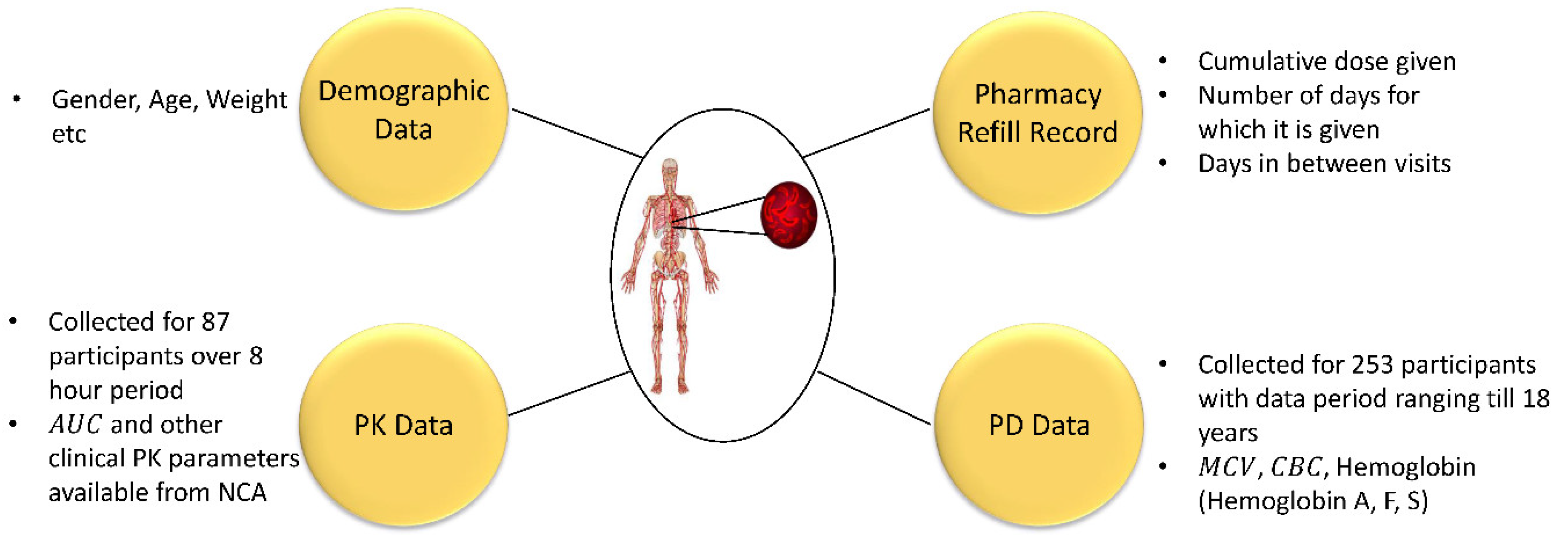
2.1. Clinical Data
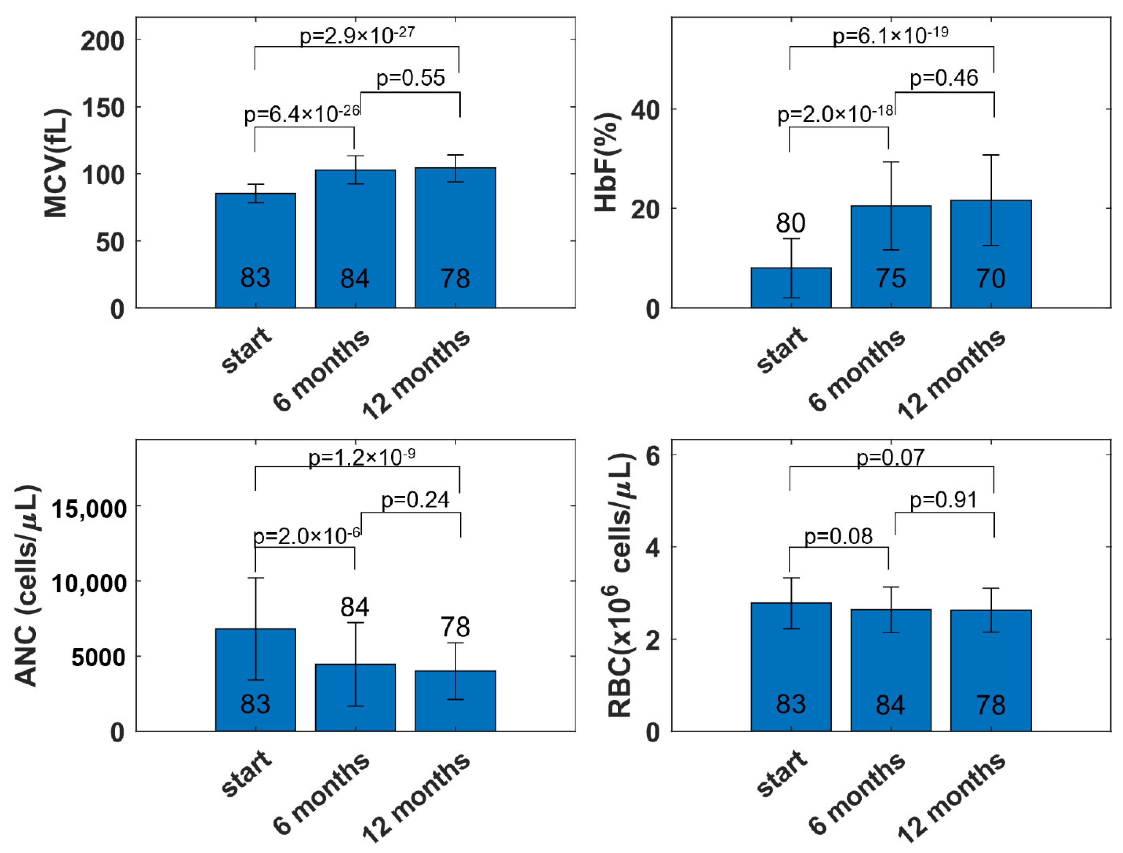
2.1.1. Observations from the Data
2.1.2. Data for Modeling
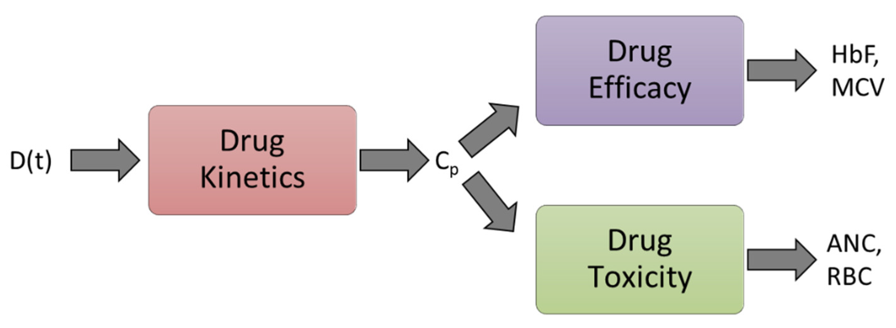
2.2. Modeling
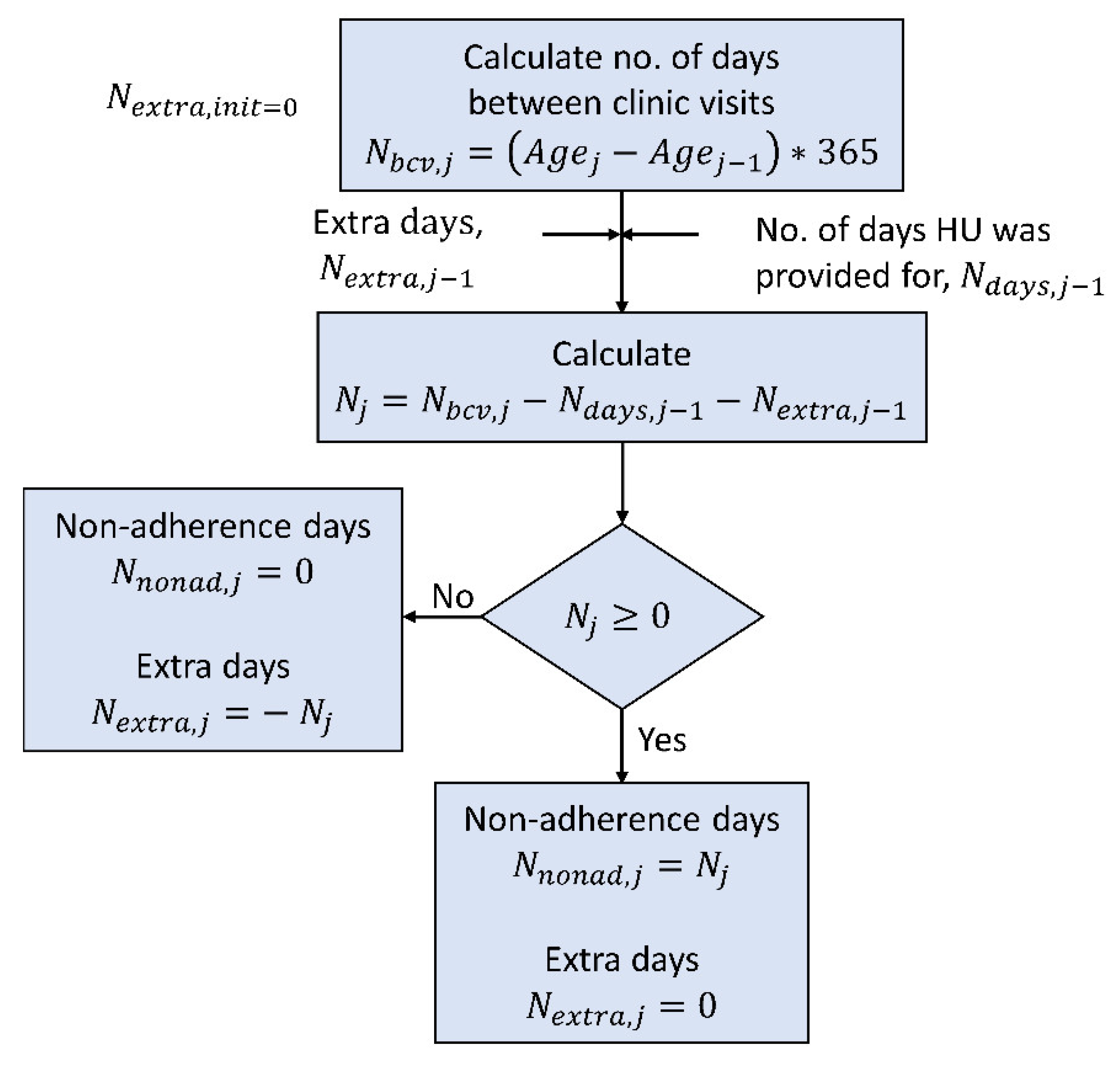
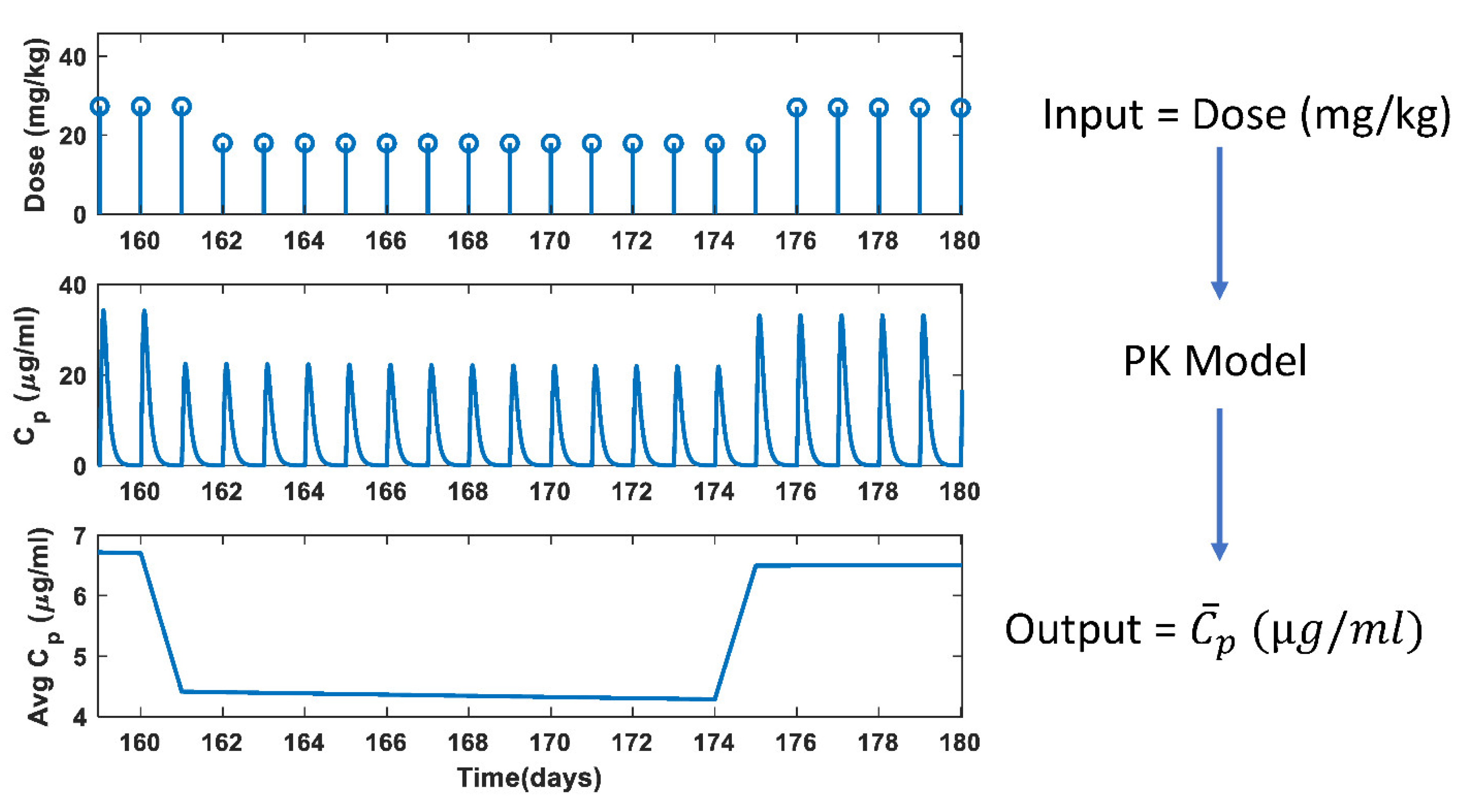
2.2.1. Dose Calculation
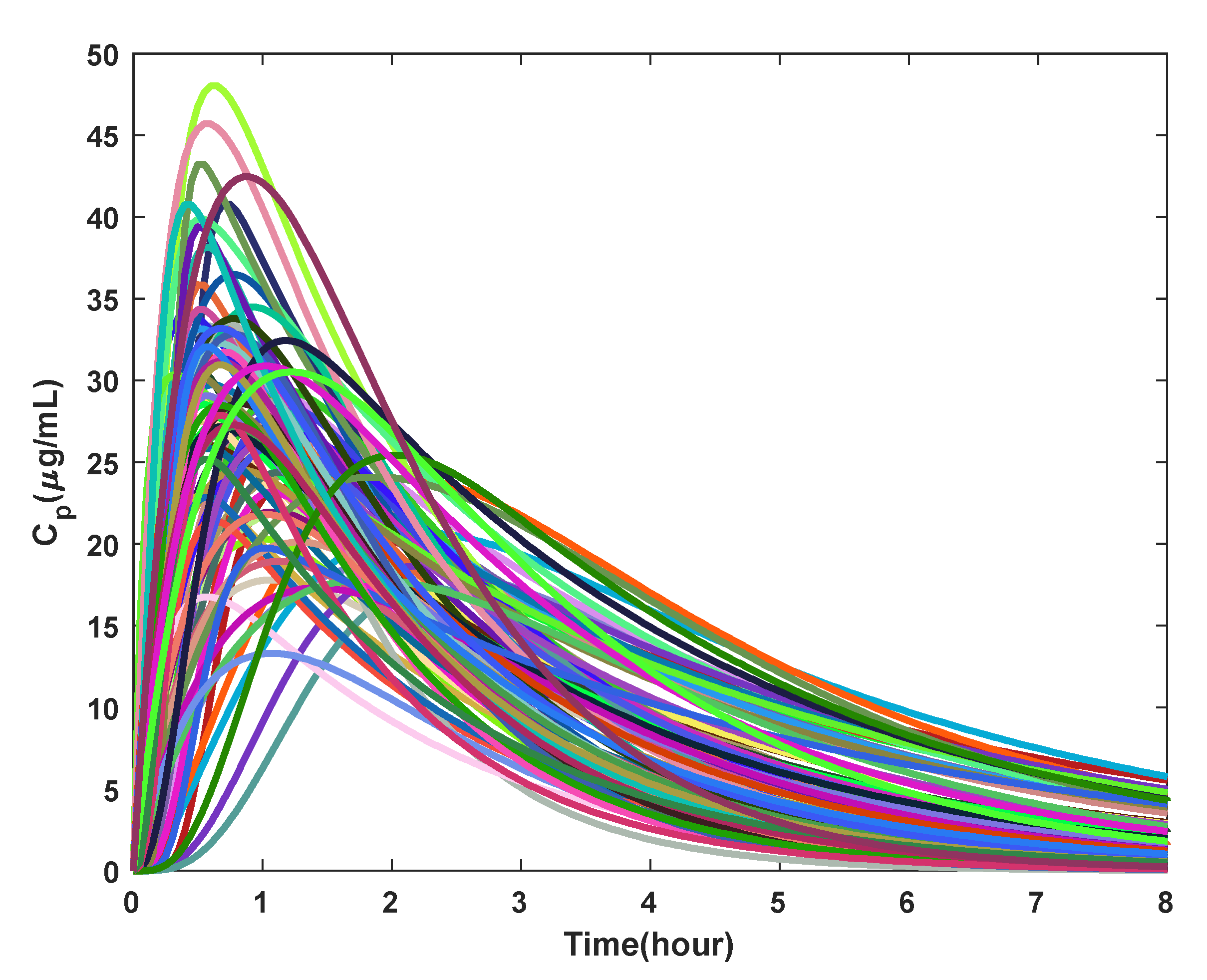
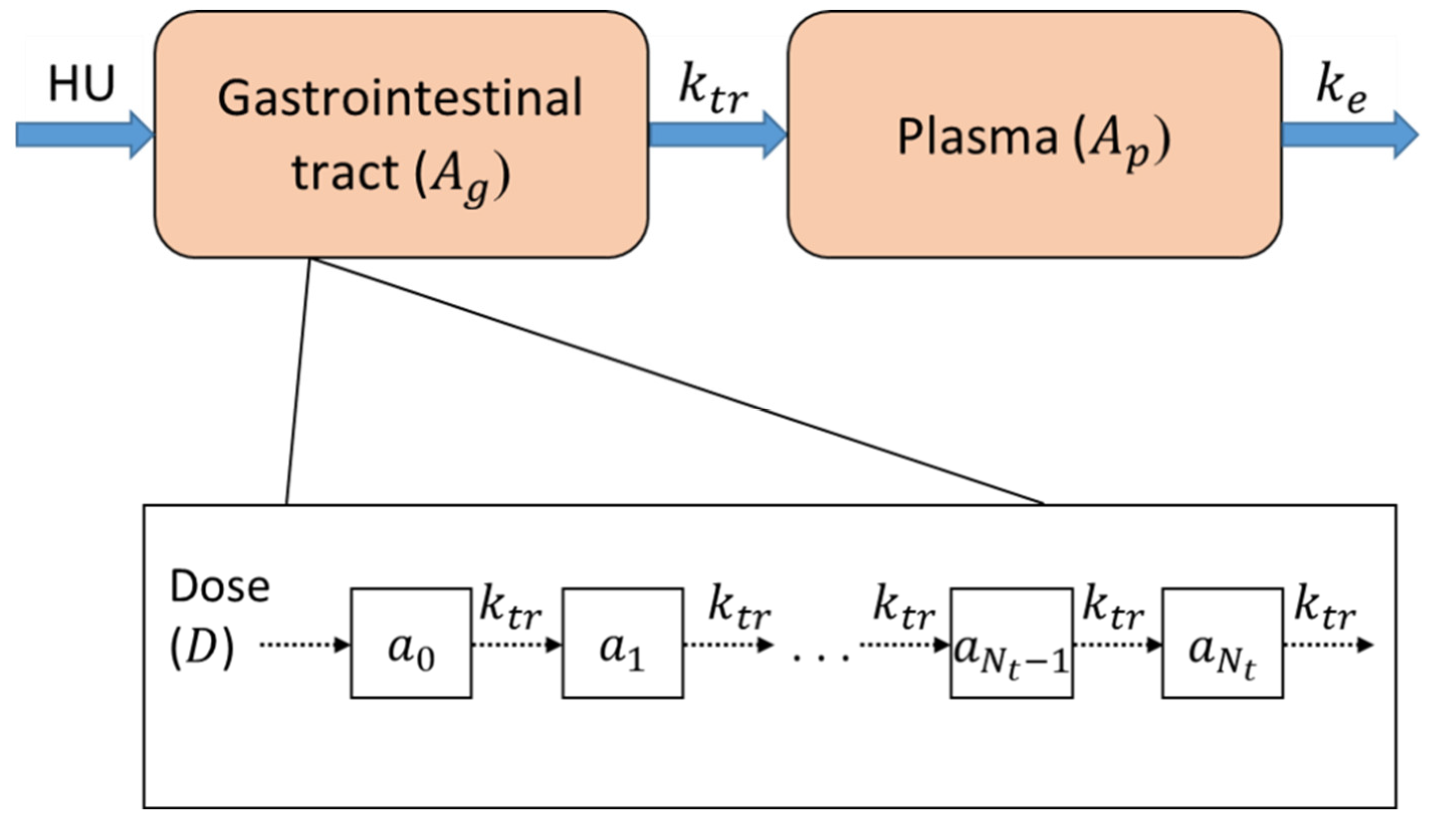
2.2.2. Pharmacokinetic Model
2.2.3. Parameter Estimation for PK Model
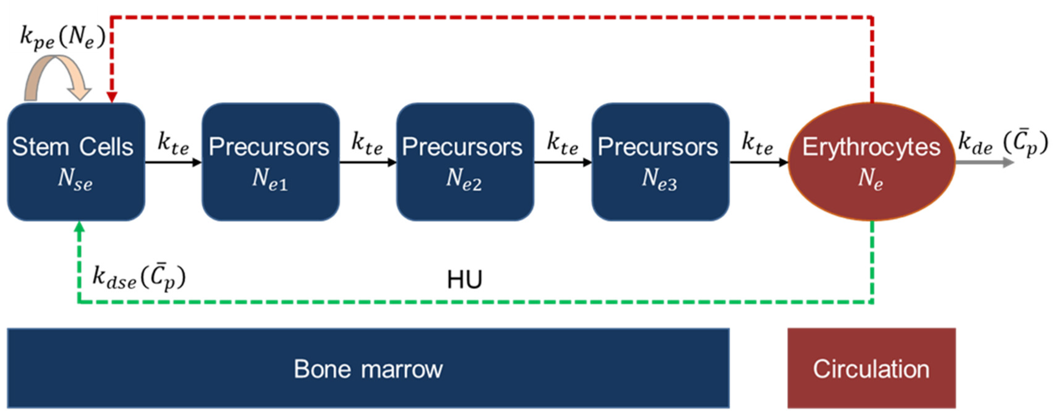
2.2.4. Erythropoiesis and MCV Model
MCV Model
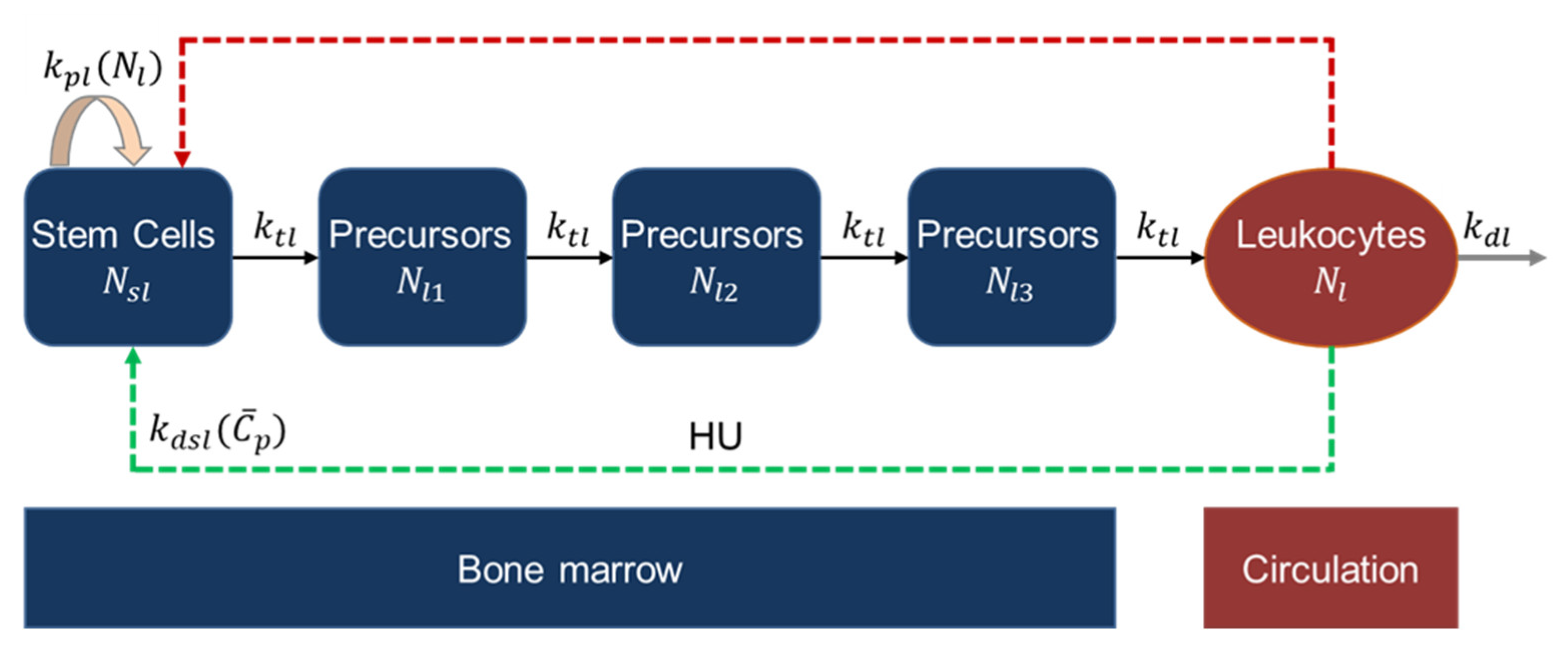
2.2.5. Leukopoiesis Model
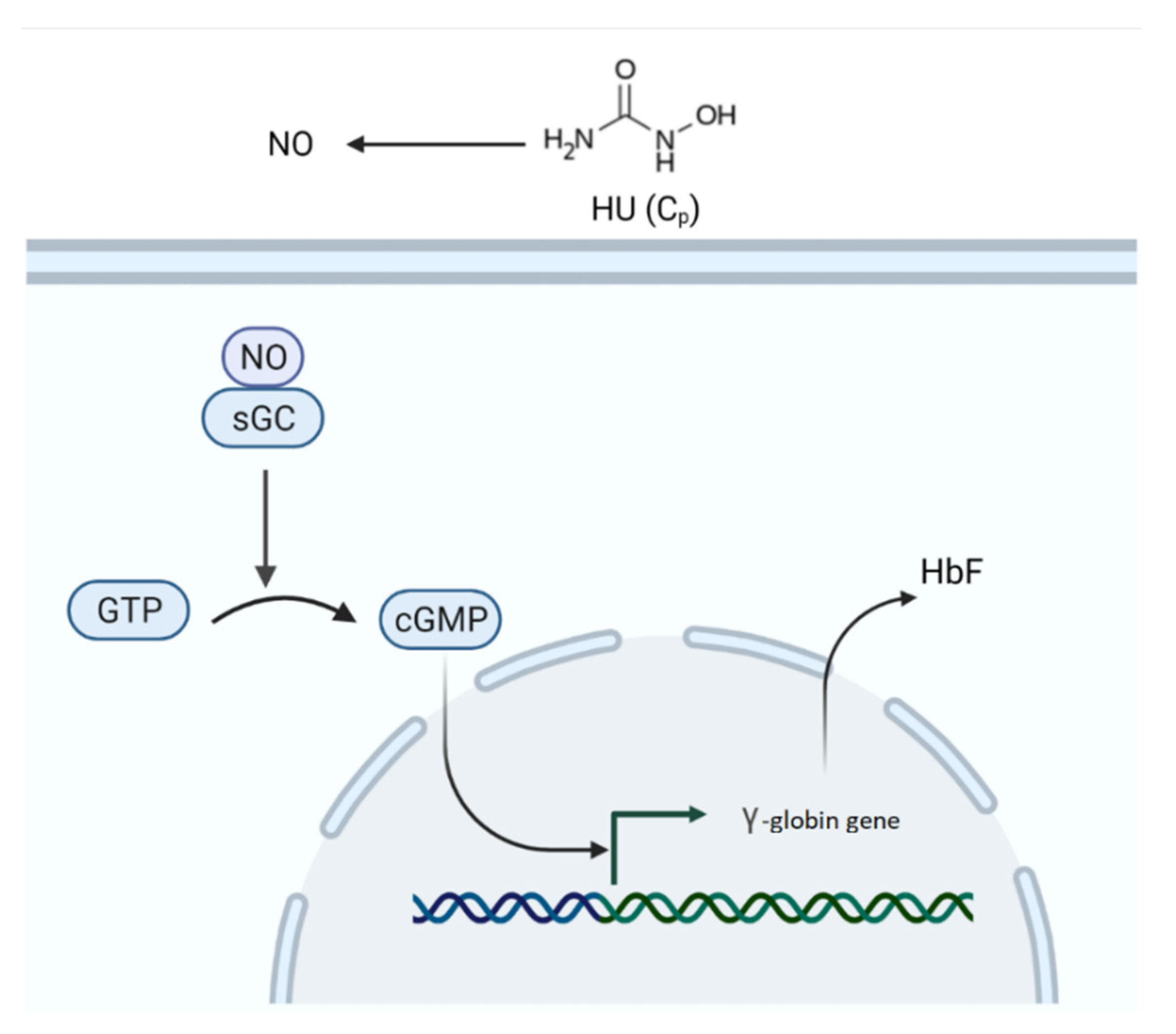
2.2.6. Fetal Hemoglobin Model
2.2.7. Parameter Estimation
3. Results
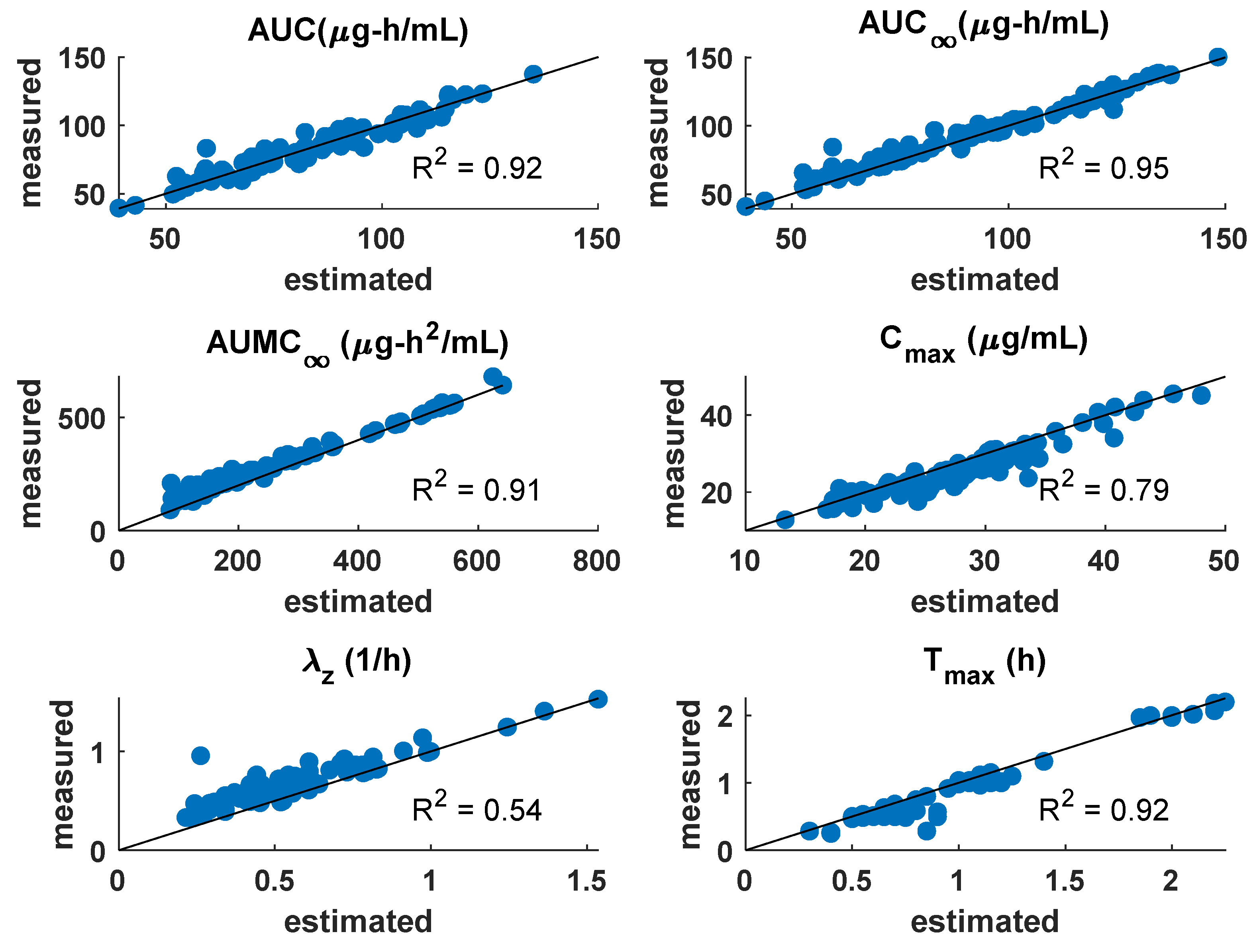
3.1. PK Model
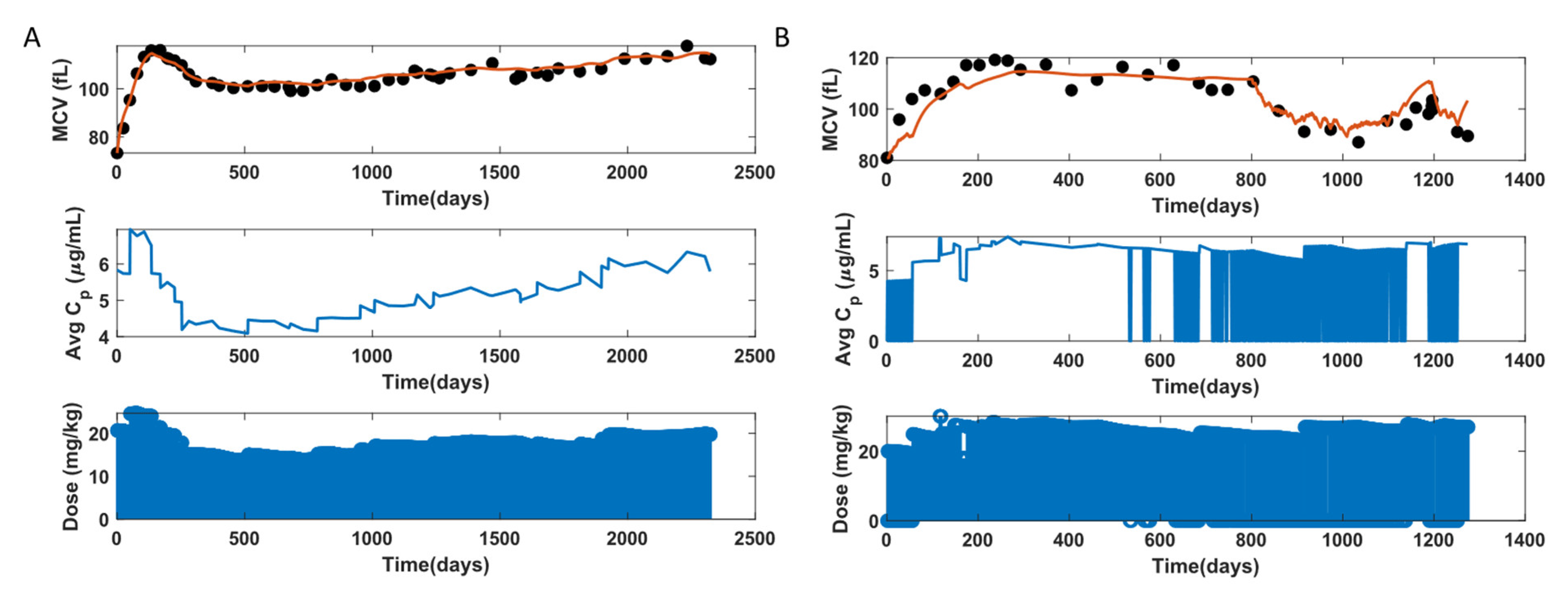
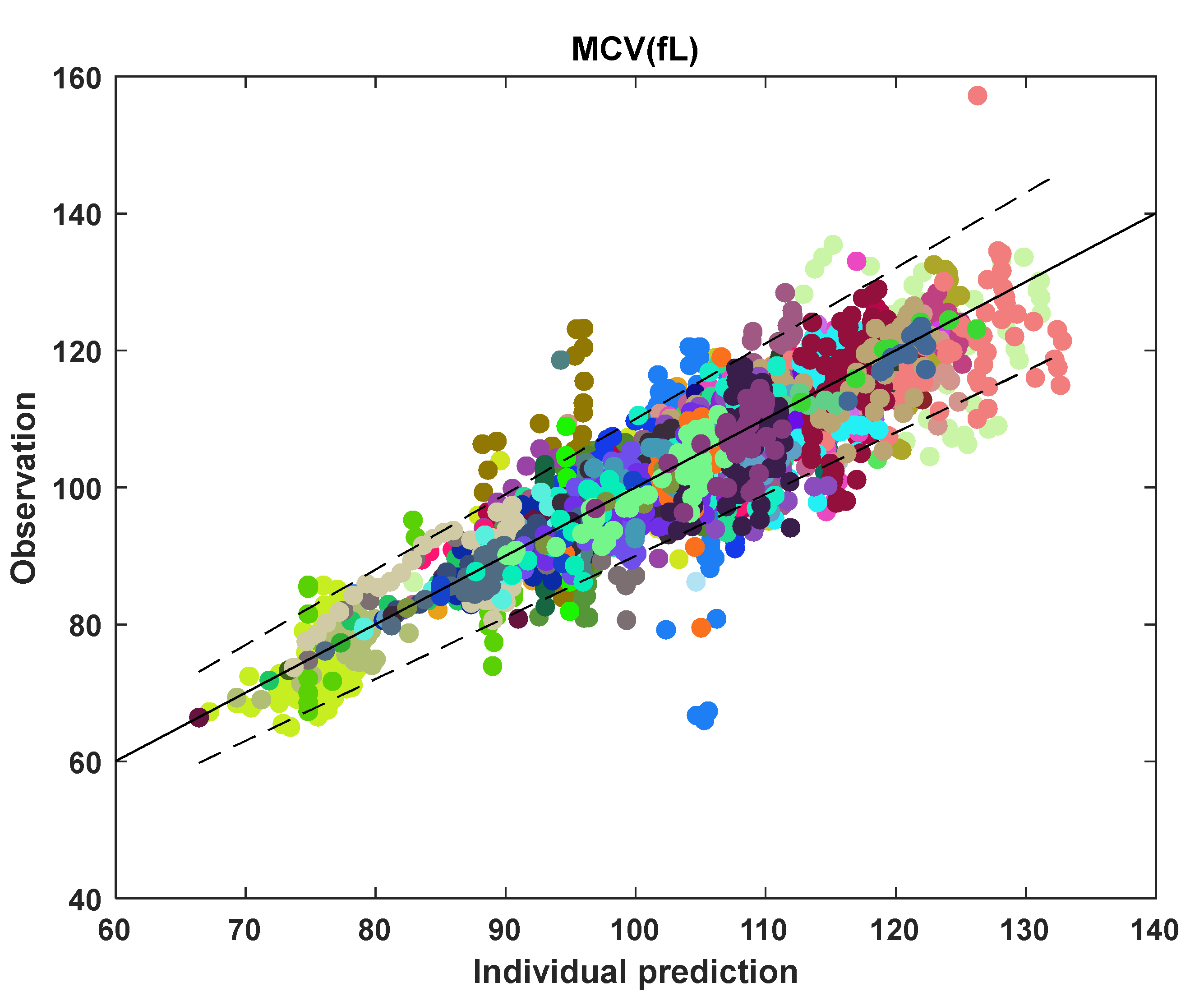
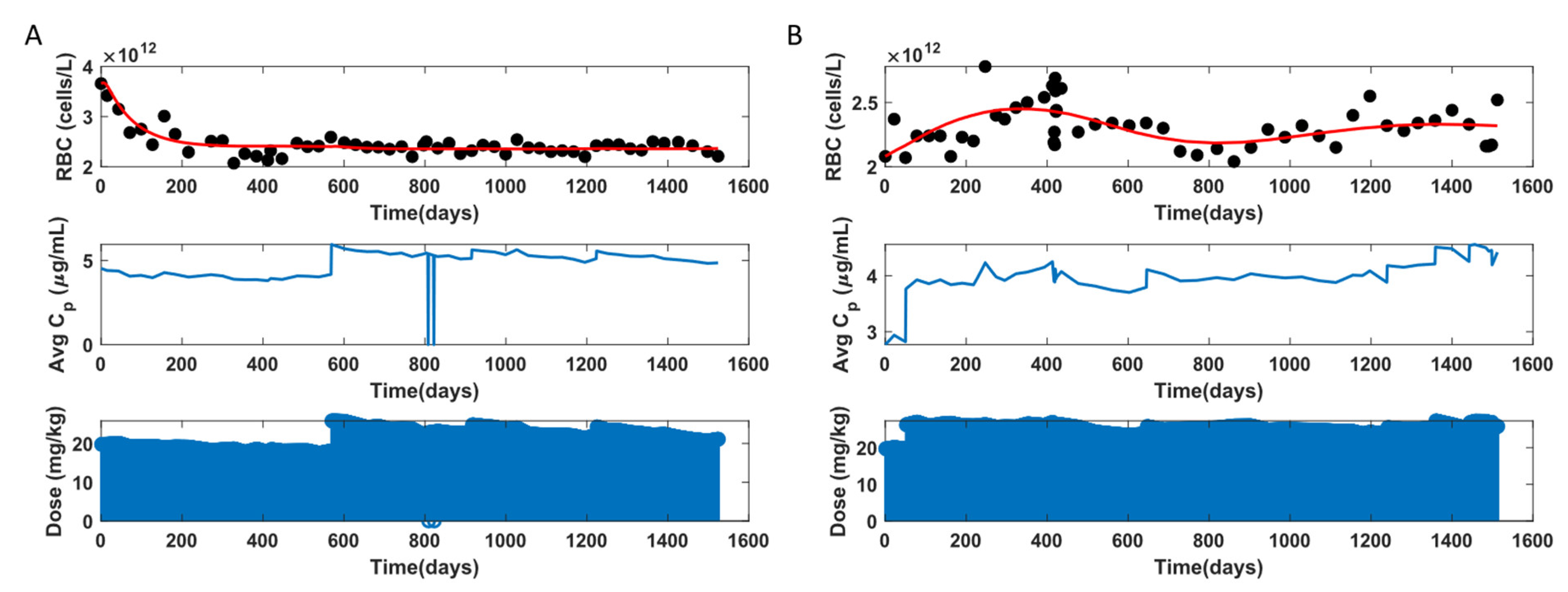
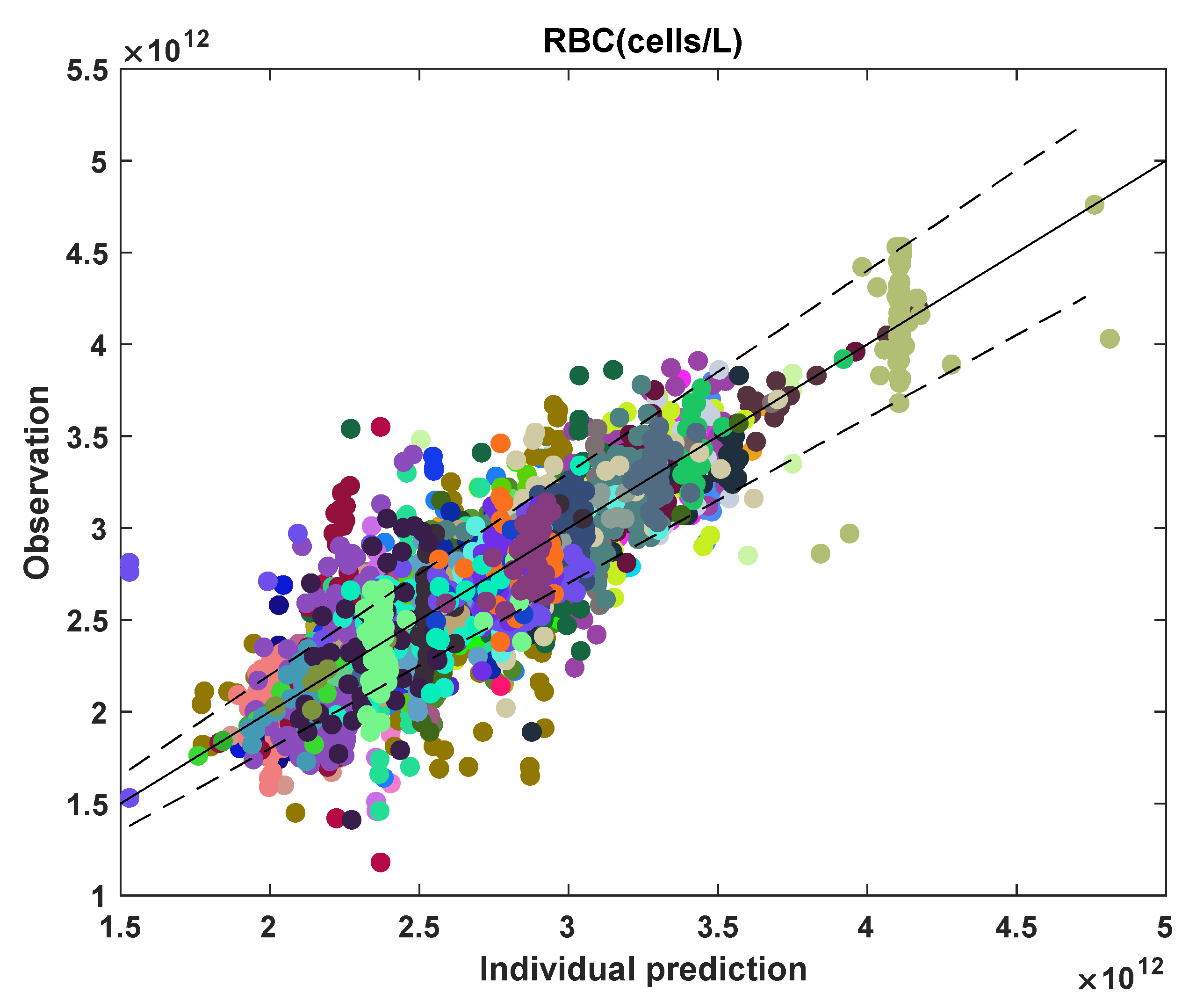
3.2. MCV and RBC Models
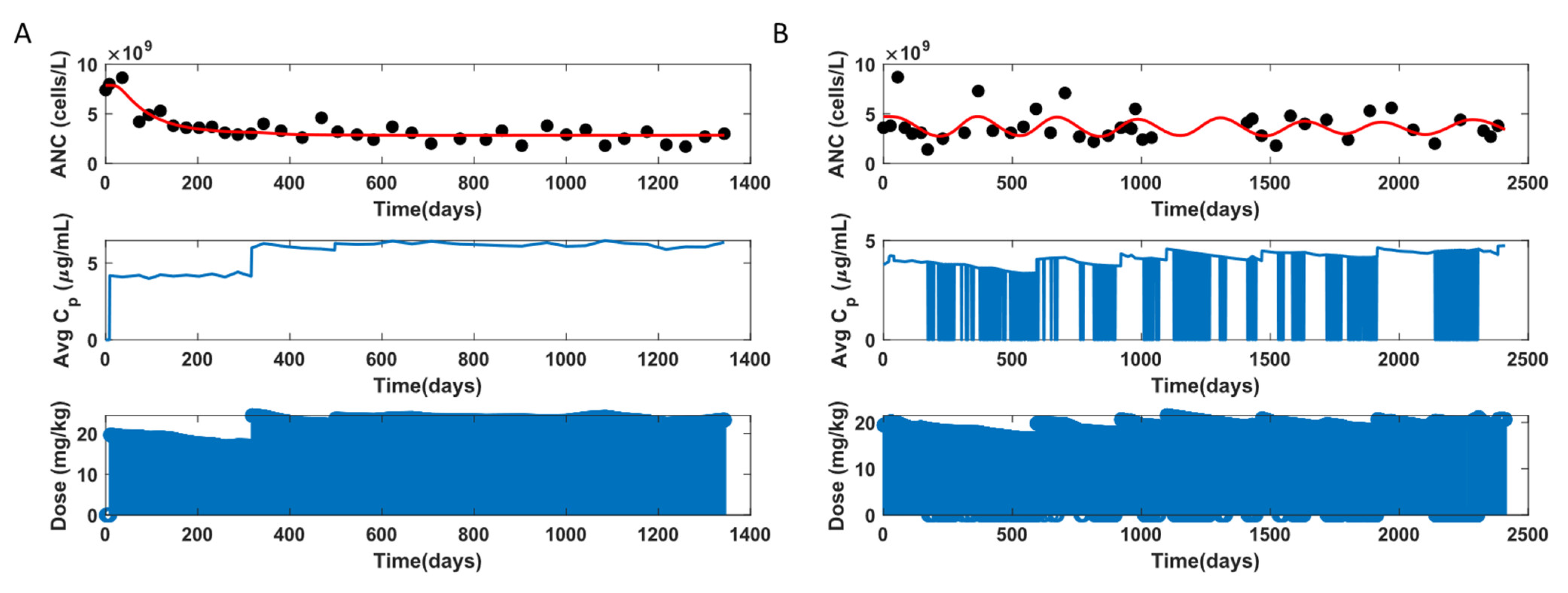
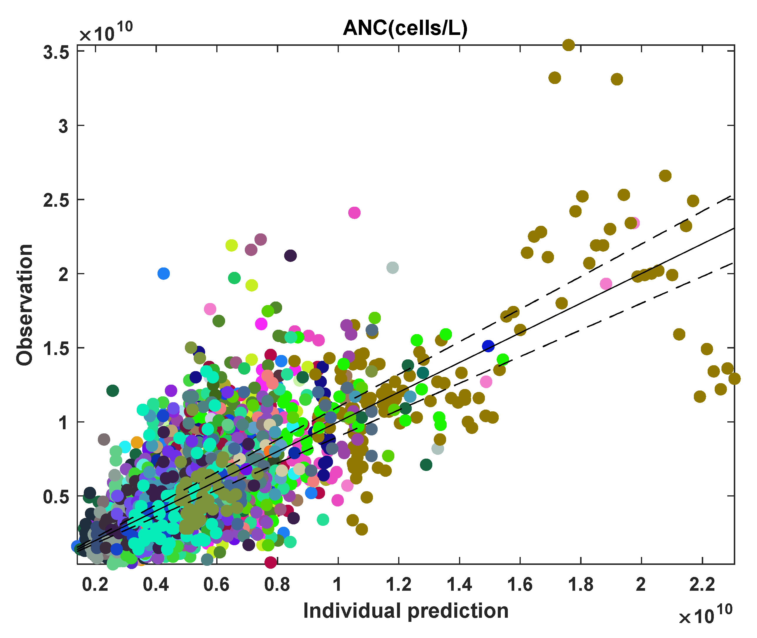
3.3. ANC Model
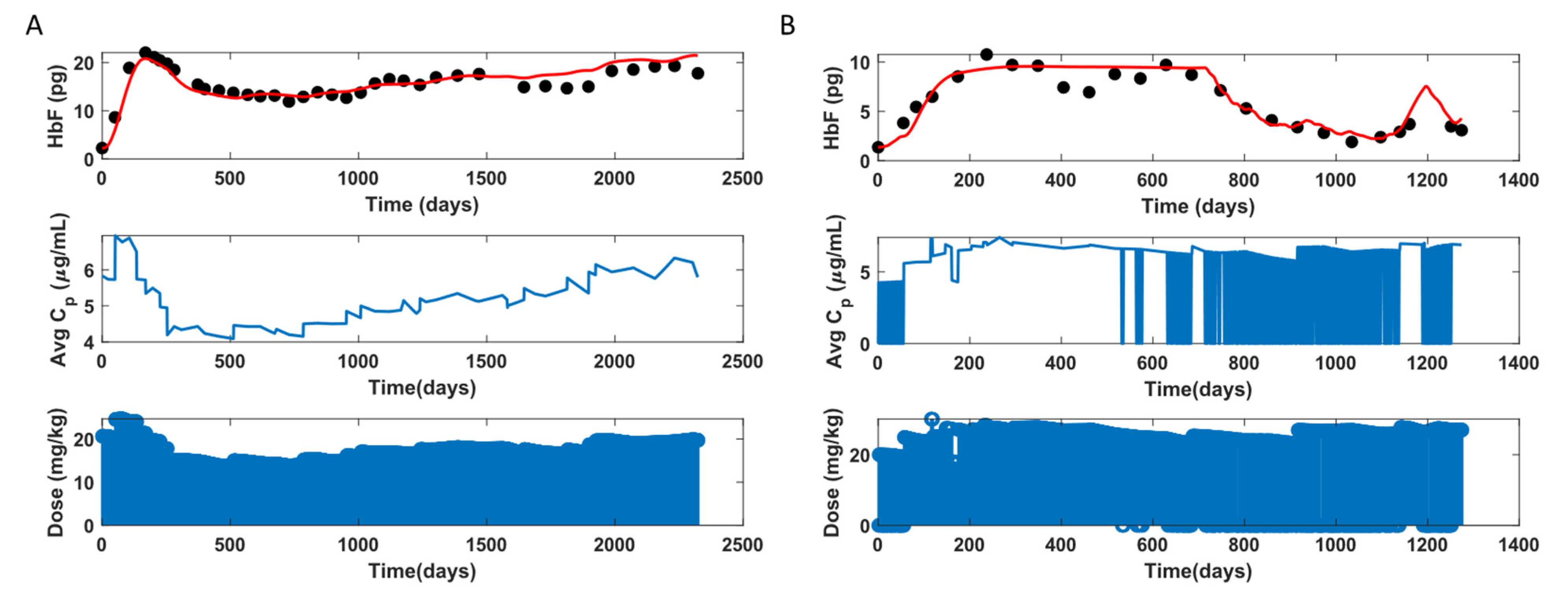
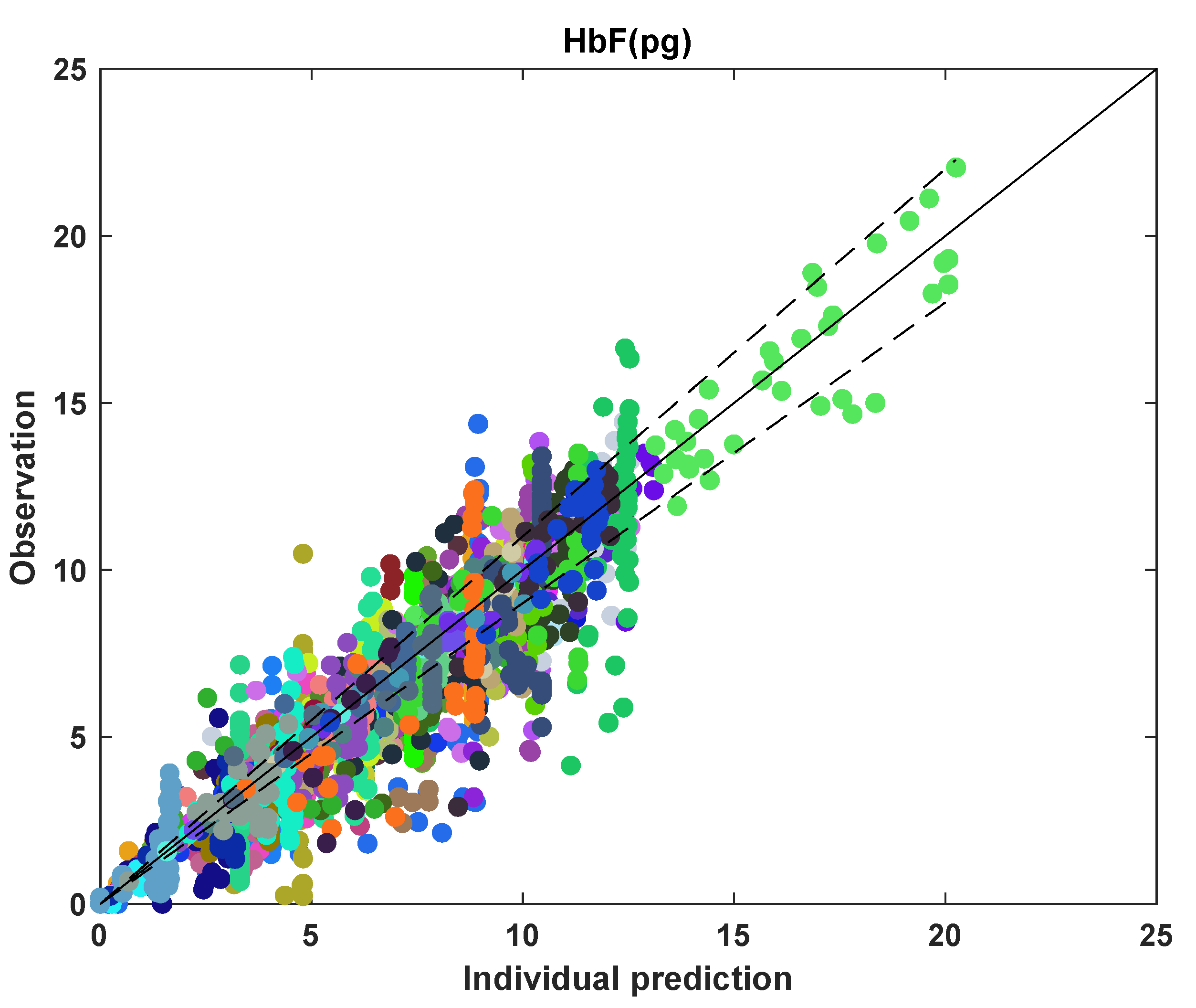
3.4. HbF Model
4. Discussion
Author Contributions
Funding
Institutional Review Board Statement
Informed Consent Statement
Data Availability Statement
Acknowledgments
Conflicts of Interest
Appendix A
- Mean Cell Fetal Hemoglobin Calculation
- 1.
- Fm (pg) is calculated by multiplying HbF (%) by mean cell hemoglobin, MCH (pg), as shown below:
- 2.
- Fm (pg) is also calculated by multiplying HbF (%) by hemoglobin, Hb (g/dL), dividing by hematocrit, HCT (%), and multiplying by MCV (fL).
- PK Compartment Modeling

- Average Drug Concentration Calculation
- MCV Calculation
References
- Sundd, P.; Gladwin, M.T.; Novelli, E.M. Pathophysiology of Sickle Cell Disease. Annu. Rev. Pathol. Mech. Dis. 2019, 14, 263–292. [Google Scholar] [CrossRef] [PubMed]
- Piel, F.B.; Steinberg, M.; Rees, D.C. Sickle Cell Disease. N. Engl. J. Med. 2017, 376, 1561–1573. [Google Scholar] [CrossRef] [PubMed] [Green Version]
- Piel, F.B.; Patil, A.P.; Howes, R.E.; Nyangiri, O.A.; Gething, P.W.; Dewi, M.; Temperley, W.H.; Williams, T.N.; Weatherall, D.J.; Hay, S.I. Global epidemiology of sickle haemoglobin in neonates: A contemporary geostatistical model-based map and population estimates. Lancet 2013, 381, 142–151. [Google Scholar] [CrossRef] [Green Version]
- Hassell, K.L. Population Estimates of Sickle Cell Disease in the U.S. Am. J. Prev. Med. 2010, 38, S512–S521. [Google Scholar] [CrossRef] [PubMed]
- Wang, W.C.; Ware, R.E.; Miller, S.T.; Iyer, R.V.; Casella, J.F.; Minniti, C.P.; Rana, S.; Thornburg, C.D.; Rogers, Z.R.; Kalpatthi, R.V.; et al. Hydroxycarbamide in very young children with sickle-cell anaemia: A multicentre, randomised, controlled trial (BABY HUG). Lancet 2011, 377, 1663–1672. [Google Scholar] [CrossRef] [Green Version]
- de Montalembert, M.; Voskaridou, E.; Oevermann, L.; Cannas, G.; Habibi, A.; Loko, G.; Joseph, L.; Colombatti, R.; Bartolucci, P.; Brousse, V.; et al. Real-Life experience with hydroxyurea in patients with sickle cell disease: Results from the prospective ESCORT-HU cohort study. Am. J. Hematol. 2021, 96, 1223–1231. [Google Scholar] [CrossRef]
- Charache, S.; Terrin, M.L.; Moore, R.D.; Dover, G.J.; Barton, F.B.; Eckert, S.V.; McMahon, R.P.; Bonds, D.R. Effect of Hydroxyurea on the Frequency of Painful Crises in Sickle Cell Anemia. N. Engl. J. Med. 1995, 332, 1317–1322. [Google Scholar] [CrossRef]
- Strouse, J.J.; Lanzkron, S.; Beach, M.C.; Haywood, C.; Park, H.; Witkop, C.; Wilson, R.F.; Bass, E.B.; Segal, J.B. Hydroxyurea for Sickle Cell Disease: A Systematic Review for Efficacy and Toxicity in Children. Pediatrics 2008, 122, 1332–1342. [Google Scholar] [CrossRef]
- Thornburg, C.D.; Files, B.A.; Luo, Z.; Miller, S.T.; Kalpatthi, R.; Iyer, R.; Seaman, P.; Lebensburger, J.; Alvarez, O.; Thompson, B.; et al. Impact of hydroxyurea on clinical events in the BABY HUG trial. Blood 2012, 120, 4304–4310. [Google Scholar] [CrossRef] [Green Version]
- Lanzkron, S.; Strouse, J.J.; Wilson, R.; Beach, M.C.; Haywood, H.; Park, H.; Witkop, C.; Bass, E.; Segal, J.B. Systematic Review: Hydroxyurea for the Treatment of Adults with Sickle Cell Disease. Ann. Intern. Med. 2008, 148, 939–955. [Google Scholar] [CrossRef]
- Brandow, A.M.; Panepinto, J.A. Hydroxyurea use in sickle cell disease: The battle with low prescription rates, poor patient compliance and fears of toxicities. Expert Rev. Hematol. 2010, 3, 255–260. [Google Scholar] [CrossRef] [PubMed] [Green Version]
- Pandey, A.; Estepp, J.H.; Ramkrishna, D. Hydroxyurea treatment of sickle cell disease: Towards a personalized model-based approach. J. Transl. Genet. Genom. 2021, 5, 22–36. [Google Scholar] [CrossRef]
- De Montalembert, M.; Bachir, D.; Hulin, A.; Gimeno, L.; Mogenet, A.; Bresson, J.L.; Macquin-Mavier, I.; Roudot-Thoraval, F.; Astier, A.; Galactéros, F. Pharmacokinetics of hydroxyurea 1000 mg coated breakable tablets and 500 mg capsules in pediatric and adult patients with sickle cell disease. Haematologica 2006, 91, 1685–1688. [Google Scholar] [PubMed]
- Ware, R.E.; Despotovic, J.M.; Mortier, N.A.; Flanagan, J.M.; He, J.; Smeltzer, M.; Kimble, A.C.; Aygun, B.; Wu, S.; Howard, T.; et al. Pharmacokinetics, pharmacodynamics, and pharmacogenetics of hydroxyurea treatment for children with sickle cell anemia. Blood 2011, 118, 4985–4991. [Google Scholar] [CrossRef] [PubMed] [Green Version]
- Estepp, J.H.; Melloni, C.; Thornburg, C.D.; Wiczling, P.; Rogers, Z.; Rothman, J.A.; Green, N.S.; Liem, R.; Do, M.A.M.B.; Crary, S.E.; et al. Pharmacokinetics and bioequivalence of a liquid formulation of hydroxyurea in children with sickle cell anemia. J. Clin. Pharmacol. 2016, 56, 298–306. [Google Scholar] [CrossRef] [PubMed] [Green Version]
- Zimmerman, S.A.; Schultz, W.H.; Davis, J.S.; Pickens, C.V.; Mortier, N.A.; Howard, T.A.; Ware, R.E. Sustained long-term hematologic efficacy of hydroxyurea at maximum tolerated dose in children with sickle cell disease. Blood 2004, 103, 2039–2045. [Google Scholar] [CrossRef]
- Kinney, T.R.; Helms, R.W.; O’Branski, E.E.; Ohene-Frempong, K.; Wang, W.; Daeschner, C.; Vichinsky, E.; Redding-Lallinger, R.; Gee, B.; Platt, O.S.; et al. Safety of hydroxyurea in children with sickle cell anemia: Results of the HUG-KIDS study, a phase I/II trial. Pediatric Hydroxyurea Group. Blood 1999, 94, 1550–1554. [Google Scholar] [CrossRef]
- Estepp, J.H.; Smeltzer, M.; Kang, G.; Li, C.; Wang, W.C.; Abrams, C.; Aygun, B.; Ware, R.E.; Nottage, K.; Hankins, J.S. A clinically meaningful fetal hemoglobin threshold for children with sickle cell anemia during hydroxyurea therapy. Am. J. Hematol. 2017, 92, 1333–1339. [Google Scholar] [CrossRef]
- Walker, A.L.; Lancaster, C.S.; Finkelstein, D.; Ware, R.E.; Sparreboom, A. Organic anion transporting polypeptide 1B transporters modulate hydroxyurea pharmacokinetics. Am. J. Physiol. Cell Physiol. 2013, 149, 1223–1229. [Google Scholar] [CrossRef] [Green Version]
- Kumkhaek, C.; Taylor, J.G.; Zhu, J.; Hoppe, C.; Kato, G.J.; Rodgers, G.P. Fetal haemoglobin response to hydroxycarbamide treatment and sar1a promoter polymorphisms in sickle cell anaemia. Br. J. Haematol. 2008, 141, 254–259. [Google Scholar] [CrossRef] [Green Version]
- Tang, D.C.; Zhu, J.; Liu, W.; Chin, K.; Sun, J.; Chen, L.; Hanover, J.A.; Rodgers, G.P. The hydroxyurea-induced small GTP-binding protein SAR modulates γ-globin gene expression in human erythroid cells. Blood 2005, 106, 3256–3263. [Google Scholar] [CrossRef] [PubMed] [Green Version]
- Ma, Q.; Wyszynski, D.F.; Farrell, J.J.; Kutlar, A.; Farrer, L.; Baldwin, C.T.; Steinberg, M. Fetal hemoglobin in sickle cell anemia: Genetic determinants of response to hydroxyurea. Pharmacogenomics J. 2007, 7, 386–394. [Google Scholar] [CrossRef] [PubMed] [Green Version]
- Yahouédéhou, S.C.M.A.; Neres, J.S.D.S.; Da Guarda, C.C.; Carvalho, S.P.; Santiago, R.P.; Figueiredo, C.V.B.; Fiuza, L.M.; Ndidi, U.S.; De Oliveira, R.M.; Fonseca, C.A.; et al. Sickle Cell Anemia: Variants in the CYP2D6, CAT, and SLC14A1 Genes Are Associated With Improved Hydroxyurea Response. Front. Pharmacol. 2020, 11, 1. [Google Scholar] [CrossRef]
- Yahouédéhou, S.C.M.A.; Adorno, E.V.; Da Guarda, C.C.; Ndidi, U.; Carvalho, S.P.; Santiago, R.P.; Aleluia, M.M.; De Oliveira, R.M.; Gonçalves, M.D.S. Hydroxyurea in the management of sickle cell disease: Pharmacogenomics and enzymatic metabolism. Pharm. J. 2018, 18, 730–739. [Google Scholar] [CrossRef] [PubMed]
- Tracewell, W.G.; Trump, D.L.; Vaughan, W.P.; Smith, D.C.; Gwilt, P.R. Population pharmacokinetics of hydroxyurea in cancer patients. Cancer Chemother. Pharmacol. 1995, 35, 417–422. [Google Scholar] [CrossRef] [PubMed]
- Villani, P.; Maserati, R.; Regazzi, M.B.; Giacchino, R.; Lori, F. Pharmacokinetics of Hydroxyurea in Patients Infected with Human Immunodeficiency Virus Type I. J. Clin. Pharmacol. 1996, 36, 117–121. [Google Scholar] [CrossRef]
- Rodriguez, G.I.; Kuhn, J.G.; Weiss, G.R.; Hilsenbeck, S.G.; Eckardt, J.R.; Thurman, A.; Rinaldi, D.A.; Hodges, S.; Von Hoff, D.D.; Rowinsky, E.K. A bioavailability and pharmacokinetic study of oral and intravenous hydroxyurea. Blood 1998, 91, 1533–1541. [Google Scholar] [CrossRef] [Green Version]
- Paule, I.; Sassi, H.; Habibi, A.; Pham, K.P.; Bachir, D.; Galactéros, F.; Girard, P.; Hulin, A.; Tod, M. Population pharmacokinetics and pharmacodynamics of hydroxyurea in sickle cell anemia patients, a basis for optimizing the dosing regimen. Orphanet J. Rare Dis. 2011, 6, 30. [Google Scholar] [CrossRef] [Green Version]
- Wiczling, P.; Liem, R.I.; Panepinto, J.A.; Garg, U.; Abdel-Rahman, S.M.; Kearns, G.L.; Neville, K.A. Population pharmacokinetics of hydroxyurea for children and adolescents with sickle cell disease. J. Clin. Pharmacol. 2014, 54, 1016–1022. [Google Scholar] [CrossRef]
- Dong, M.; McGann, P.T.; Mizuno, T.; Ware, R.E.; Vinks, A.A. Development of a pharmacokinetic-guided dose individualization strategy for hydroxyurea treatment in children with sickle cell anaemia. Br. J. Clin. Pharmacol. 2016, 81, 742–752. [Google Scholar] [CrossRef] [Green Version]
- McGann, P.T.; Niss, O.; Dong, M.; Marahatta, A.; Howard, T.A.; Mizuno, T.; Lane, A.; Kalfa, T.; Malik, P.; Quinn, C.T.; et al. Robust clinical and laboratory response to hydroxyurea using pharmacokinetically guided dosing for young children with sickle cell anemia. Am. J. Hematol. 2019, 94, 871–879. [Google Scholar] [CrossRef] [PubMed]
- Lard, L.R.; Mul, F.P.J.; de Haas, M.; Roos, D.; Duits, A.J. Neutrophil activation in sickle cell disease. J. Leukoc. Biol. 1999, 66, 411–415. [Google Scholar] [CrossRef] [PubMed]
- Turhan, A.; Weiss, L.A.; Mohandas, N.; Coller, B.S.; Frenette, P.S. Primary role for adherent leukocytes in sickle cell vascular occlusion: A new paradigm. Proc. Natl. Acad. Sci. USA 2002, 99, 3047–3051. [Google Scholar] [CrossRef] [PubMed] [Green Version]
- Ballas, S.; Marcolina, M.; Dover, G.; Barton, F. Erythropoietic activity in patients with sickle cell anaemia before and after treatment with hydroxyurea. Br. J. Haematol. 1999, 105, 491–496. [Google Scholar] [CrossRef] [PubMed]
- MATLAB. Version: 9.9.0.1467703 (R2020b); The MathWorks Inc.: Natick, MA, USA, 2020. [Google Scholar]
- Čokić, V.; Smith, R.D.; Beleslin-Cokic, B.B.; Njoroge, J.M.; Miller, J.L.; Gladwin, M.T.; Schechter, A.N. Hydroxyurea induces fetal hemoglobin by the nitric oxide-dependent activation of soluble guanylyl cyclase. J. Clin. Investig. 2003, 111, 231–239. [Google Scholar] [CrossRef] [PubMed] [Green Version]
- Ikuta, T.; Ausenda, S.; Cappellini, M.D. Mechanism for fetal globin gene expression: Role of the soluble guanylate cyclase-cGMP-dependent protein kinase pathway. Proc. Natl. Acad. Sci. USA 2001, 98, 1847–1852. [Google Scholar] [CrossRef]
- Pace, B.S.; Qian, X.-H.; Sangerman, J.; Ofori-Acquah, S.; Baliga, B.; Han, J.; Critz, S.D. p38 MAP kinase activation mediates γ-globin gene induction in erythroid progenitors. Exp. Hematol. 2003, 31, 1089–1096. [Google Scholar] [CrossRef]
- Savic, R.M.; Jonker, D.M.; Kerbusch, T.; Karlsson, M.O. Implementation of a transit compartment model for describing drug absorption in pharmacokinetic studies. J. Pharmacokinet. Pharmacodyn. 2007, 34, 711–726. [Google Scholar] [CrossRef]
- Nadler, S.B.; Hidalgo, J.H.; Bloch, T. Prediction of blood volume in normal human adults. Surgery 1962, 51, 224–232. [Google Scholar]
- Hauser, R.G.; Cheng, C.; Ryder, A. Blood Volume Calculation. Available online: https://www.mdcalc.com/blood-volume-calculation#evidence (accessed on 11 February 2022).
- Nedea, D. Pediatric Blood Volume Calculator. Available online: https://www.mdapp.co/pediatric-blood-volume-calculator-538/#here (accessed on 11 February 2022).
- Barnes, D.J.; Melo, J.V. Management of chronic myeloid leukemia: Targets for molecular therapy. Semin. Hematol. 2003, 40, ashem0400034. [Google Scholar] [CrossRef]
- Jayachandran, D.; Rundell, A.E.; Hannemann, R.E.; Vik, T.; Ramkrishna, D. Optimal Chemotherapy for Leukemia: A Model-Based Strategy for Individualized Treatment. PLoS ONE 2014, 9, e109623. [Google Scholar] [CrossRef] [PubMed] [Green Version]
- Bunn, H.F. Erythropoietin. Cold Spring Harb. Perspect. Med. 2013, 3, a011619. [Google Scholar] [CrossRef] [PubMed] [Green Version]
- Haase, V.H. Hypoxic regulation of erythropoiesis and iron metabolism. Am. J. Physiol. Physiol. 2010, 299, F1–F13. [Google Scholar] [CrossRef] [PubMed] [Green Version]
- Föller, M.; Huber, S.M.; Lang, F. Erythrocyte programmed cell death. IUBMB Life 2008, 60, 661–668. [Google Scholar] [CrossRef]
- Kaushansky, K. Hematopoietic Stem Cells, Progenitors, and Cytokines. In Williams Hematology, 9th ed.; Kaushansky, K., Lichtman, M.A., Prchal, J.T., Levi, M.M., Press, O.W., Burns, L.J., Caligiuri, M., Eds.; McGraw Hill: New York, NY, USA, 2015; Available online: https://accessmedicine.mhmedical.com/content.aspx?bookid=1581§ionid=94302625 (accessed on 11 February 2022).
- Ogawa, M. Differentiation and proliferation of hematopoietic stem cells. Blood 1993, 81, 2844–2853. [Google Scholar] [CrossRef] [Green Version]
- Davis, L.R. Changing blood picture in sickle-cell anaemia from shortly after birth to adolescence. J. Clin. Pathol. 1976, 29, 898–901. [Google Scholar] [CrossRef] [Green Version]
- Forget, B.G. Molecular Basis of Hereditary Persistence of Fetal Hemoglobin. Ann. N. Y. Acad. Sci. 1998, 850, 38–44. [Google Scholar] [CrossRef]
- Sokolova, A.; Mararenko, A.; Rozin, A.; Podrumar, A.; Gotlieb, V. Hereditary persistence of hemoglobin F is protective against red cell sickling. A case report and brief review. Hematol. Stem Cell Ther. 2019, 12, 215–219. [Google Scholar] [CrossRef]
- Thein, S.L.; Menzel, S.; Lathrop, M.; Garner, C. Control of fetal hemoglobin: New insights emerging from genomics and clinical implications. Hum. Mol. Genet. 2009, 18, R216–R223. [Google Scholar] [CrossRef] [Green Version]
- Labie, D.; Pagnier, J.; Lapoumeroulie, C.; Rouabhi, F.; Dunda-Belkhodja, O.; Chardin, P.; Beldjord, C.; Wajcman, H.; E Fabry, M.; Nagel, R.L. Common haplotype dependency of high G gamma-globin gene expression and high Hb F levels in beta-thalassemia and sickle cell anemia patients. Proc. Natl. Acad. Sci. USA 1985, 82, 2111–2114. [Google Scholar] [CrossRef] [Green Version]
- Kovacic, P. Hydroxyurea (therapeutics and mechanism): Metabolism, carbamoyl nitroso, nitroxyl, radicals, cell signaling and clinical applications. Med. Hypotheses 2011, 76, 24–31. [Google Scholar] [CrossRef] [PubMed]
- Lou, T.-F.; Singh, M.; Mackie, A.; Li, W.; Pace, B.S. Hydroxyurea Generates Nitric Oxide in Human Erythroid Cells: Mechanisms for γ-Globin Gene Activation. Exp. Biol. Med. 2009, 234, 1374–1382. [Google Scholar] [CrossRef] [PubMed] [Green Version]
- Huang, J.; Kim-Shapiro, D.B.; King, S.B. Catalase-Mediated Nitric Oxide Formation from Hydroxyurea. J. Med. Chem. 2004, 47, 3495–3501. [Google Scholar] [CrossRef] [PubMed]
- Huang, J.; Sommers, E.M.; Kim-Shapiro, D.B.; King, S.B. Horseradish Peroxidase Catalyzed Nitric Oxide Formation from Hydroxyurea. J. Am. Chem. Soc. 2002, 124, 3473–3480. [Google Scholar] [CrossRef] [PubMed]
- Ermentrout, B.; Mahajan, A. Simulating, Analyzing, and Animating Dynamical Systems: A Guide to XPPAUT for Researchers and Students. Appl. Mech. Rev. 2003, 56, B53. [Google Scholar] [CrossRef]
- Frenette, P.S. Sickle cell vaso-occlusion: Multistep and multicellular paradigm. Curr. Opin. Hematol. 2002, 9, 101–106. [Google Scholar] [CrossRef] [PubMed]
- Thein, S.L.; Craig, J. Genetics of Hb F/F Cell Variance in Adults and Heterocellular Hereditary Persistence of Fetal Hemoglobin. Hemoglobin 1998, 22, 401–414. [Google Scholar] [CrossRef]


| Demographics | |||
|---|---|---|---|
| Starting age of HU treatment (years) | 10.12 (4.72) Mean (SD) | ||
| Male/Female | 54/31 | ||
| Clinical PK parameters | Mean (SD) | ||
| (µg∙h/mL) | 85.79 (19.64) | ||
| (µg∙h/mL) | 92.98 (23.37) | ||
| (h) | 3.17 (0.78) | ||
| (h) | 0.82 (0.47) | ||
| (µg/mL) | 26.13 (6.83) | ||
| (h−1) | 0.65 (0.23) | ||
| PD variables | At baseline Mean (SD) | After 6 months of treatment Mean (SD) | After 12 months of treatment Mean (SD) |
| MCV (fL) | 85.34 (6.958) | 103.1 (10.46) | 104.1 (10.06) |
| MCH (pg) | 29.76 (2.842) | 35.51 (3.866) | 36 (3.876) |
| HCT (%) | 23.46 (3.649) | 26.9 (4.102) | 27.12 (3.858) |
| Hb (g/dL) | 8.151 (1.143) | 9.246 (1.332) | 9.364 (1.279) |
| HbF (%) | 8.004 (5.978) | 20.54 (8.854) | 21.65 (9.129) |
| HbS (%) | 72.92 (20.09) | 68.65 (9.441) | 67.34 (11.99) |
| ANC (cells/µL) | 6814 (3384) | 4449 (2779) | 4007 (1891) |
| cells/µL) | 13.51 (4.981) | 9.114 (3.273) | 8.418 (2.864) |
| cells/µL) | 0.2711 (0.0958) | 0.1563 (0.0840) | 0.1522 (0.0615) |
| cells/µL) | 2.777 (0.5517) | 2.636 (0.4918) | 2.628 (0.4709) |
| Parameter | Mean (SD) |
|---|---|
| 0.12 (0.04) | |
| (h−1) | 5.02 (2.61) |
| 1.14 (1.08) | |
| (h−1) | 0.54 (0.26) |
| (L) | 1.77 (0.88) |
| Parameter | Median | 1st Quartile | 3rd Quartile |
|---|---|---|---|
| (cells/L/day) | 2.10 × 10¹² | 1.30 × 10¹¹ | 1.90 × 10¹⁴ |
| (cells/L) | 2.20 × 10¹¹ | 7.10 × 10¹⁰ | 1.10 × 10¹² |
| 1.6 | 0.52 | 3.3 | |
| (1/day) | 0.17 | 0.02 | 0.71 |
| (µM) | 0.43 | 0.01 | 4.4 |
| (1/day) | 0.2 | 0.05 | 0.37 |
| (1/day) | 0.03 | 0.01 | 0.06 |
| (µM) | 310 | 62 | 860 |
| (fL/µM) | 0.37 | 0.23 | 0.51 |
| Parameter | Median | 1st Quartile | 3rd Quartile |
|---|---|---|---|
| (cells/L/day) | 1.10 × 10¹² | 3.30 × 10¹⁰ | 1.80 × 10¹⁴ |
| (cells/L) | 4.70 × 10⁸ | 1.50 × 10⁸ | 1.20 × 10⁹ |
| 3.5 | 2 | 4.3 | |
| (1/day) | 0.16 | 0.04 | 1.2 |
| (µM) | 0.3 | 0.01 | 30 |
| (1/day) | 0.09 | 0.03 | 0.32 |
| (1/day) | 0.13 | 0.03 | 0.45 |
| Parameter | Median | 1st Quartile | 3rd Quartile |
|---|---|---|---|
| (µM/day) | 1.2 | 0.05 | 3.5 |
| (µM) | 27 | 4 | 110 |
| (1/day) | 0.03 | 0.01 | 0.06 |
| (pg/day) | 0.16 | 0.04 | 0.64 |
| (pg/day) | 1.5 | 0.3 | 4.3 |
| (µM) | 13 | 2.2 | 45 |
| 3.2 | 1.6 | 4.5 | |
| (1/day) | 0.07 | 0.02 | 0.3 |
Publisher’s Note: MDPI stays neutral with regard to jurisdictional claims in published maps and institutional affiliations. |
© 2022 by the authors. Licensee MDPI, Basel, Switzerland. This article is an open access article distributed under the terms and conditions of the Creative Commons Attribution (CC BY) license (https://creativecommons.org/licenses/by/4.0/).
Share and Cite
Pandey, A.; Estepp, J.H.; Raja, R.; Kang, G.; Ramkrishna, D. Mathematical Modeling of Hydroxyurea Therapy in Individuals with Sickle Cell Disease. Pharmaceutics 2022, 14, 1065. https://0-doi-org.brum.beds.ac.uk/10.3390/pharmaceutics14051065
Pandey A, Estepp JH, Raja R, Kang G, Ramkrishna D. Mathematical Modeling of Hydroxyurea Therapy in Individuals with Sickle Cell Disease. Pharmaceutics. 2022; 14(5):1065. https://0-doi-org.brum.beds.ac.uk/10.3390/pharmaceutics14051065
Chicago/Turabian StylePandey, Akancha, Jeremie H. Estepp, Rubesh Raja, Guolian Kang, and Doraiswami Ramkrishna. 2022. "Mathematical Modeling of Hydroxyurea Therapy in Individuals with Sickle Cell Disease" Pharmaceutics 14, no. 5: 1065. https://0-doi-org.brum.beds.ac.uk/10.3390/pharmaceutics14051065